A Dual-Wavelength Ocean Lidar for Vertical Profiling of Oceanic Backscatter and Attenuation

Abstract

Ocean water column information profiles are essential for ocean research. Currently, water column profiles are typically obtained by ocean lidar instruments, including spaceborne, airborne and shipborne lidar, most of which are equipped with a 532 nm laser; however, blue wavelength penetrates more for open ocean detection. In this paper, we present a novel airborne dual-wavelength ocean lidar (DWOL), equipped with a 532 and 486 nm laser that can operate simultaneously. This instrument was designed to compare the performance of 486 and 532 nm lasers in a single detection area and to provide a reference for future spaceborne oceanic lidar (SBOL) design. Airborne and shipborne experiments were conducted in the South China Sea. Results show that—for a 500-frame accumulation—the 486 nm channel obtained volume profiles from a depth of approximately 100 m. In contrast, the vertical profiles obtained by the 532 nm channel only reached in a depth of 75 m, which was approximately 25% less than that of 486 m channel in the same detection area. Results from the inverse lidar attenuation coefficient $\alpha (z)$ for the DWOL show that the maximum value of $\alpha (z)$ ranged from 40 to 80 m, which was consistent with the chlorophyll-scattering layer (CSL) distribution measured by the shipborne instrument. Additionally, ${\alpha }_{486}(z)$ decreased for depth beyond 80 m, indicating that the 486 nm laser can potentially penetrate the entire CSL.

1. Introduction

Over the past decades, both passive and active ocean optical remote sensing technologies have revolutionized our understanding of the ocean. Passive remote sensing technology is commonly used in the research of the carbon cycle for the upper ocean on a global scale [1,2]. However, this type of system can only obtain weighted integral information at a limited depth. Vertical profile information such as chlorophyll profiles or salinity data, is very important for understanding oceanic physical-biogeochemical processes, ocean primary production and other aspects of the ocean environment [3,4,5]. This type of information can be obtained via active ocean remote sensing technology, such as shipborne and airborne ocean lidar for small-region detection and spaceborne ocean lidar (SBOL) for large-scale detection [6,7].

Current ocean lidar systems are typically equipped with a 532 nm lasers, as these lasers work best for coastal waters detection [8,9,10]. The 532 nm lasers are relatively low-cost, robust lasing system that can provide high-energy pulses for coastal waters detection. However, for open ocean water, shorter wavelengths are optimal, due to the reduction of colored dissolved organic material (CDOM), the decrease of detritus and the decreasing concentration of phytoplankton. Some researchers have recommended a wavelength of 490 nm for open ocean water detection [11]. To estimate the detection performance of shorter wavelengths near 490 nm and to improve the performance of daytime working lidar systems, we designed a novel dual-wavelength ocean lidar (DWOL) system equipped with 486 and 532 nm lasers. The 486-nm band coincides with one of the Fraunhofer dark lines [12,13]; thus, the background noise for this band will be lower than that of other wavelength band. Additionally, some researchers have studied the advantage of multi-wavelength lidar for improving the depth resolutions [14], in this study, the two wavelengths of 532 and 486 nm will be utilized to explore the advantages of multi-wavelength lidar systems for natural water detection [15,16,17].

Due to the substantial attenuation that occurs from the ocean surface to a depth of tens of meters, one of the challenges encountered in active ocean detection is the limited dynamic ranges of traditional detectors. In the DWOL system, we utilized a photomultiplier tube (PMT) as the receiving detector. Additionally, the analog detection mode and the photon-counting mode of the PMT are used simultaneously to increase the dynamic range. However, when working in the photon-counting mode, the PMT detector generates a series of pseudo-counting photons, termed the after-pulse count (APC), after a strong returning pulse signal is received. This noise can cause substantial errors in the signal inversion results [18,19,20,21]. Some studies have aimed to eliminate this effect in atmospheric and oceanic detection [22,23,24,25]. In this study, we developed a new correction method to reduce the effects of the APC.

Shipborne and airborne lidars are commonly used in active local ocean detection; in contrast for active large-scale ocean detection, a spaceborne platform is the optimal choice. Over the past decades, the Ice, Cloud and land Elevation Satellite (ICESat) mission [26] and the Cloud Aerosol Lidar and Infrared Pathfinder Satellite Observation (CALIPSO) [6] have demonstrated the feasibility of using spaceborne lidar for ocean detection.

The DWOL system was primarily designed to estimate the detection performance of the 486 nm laser compared with 532 nm laser when working far from the coast. Additionally, as a scaled experiment, the DWOL system provides a reference for future SBOL design [27].

In this study, we report on the design of a DWOL system as well as airborne and shipborne measurements experiments conducted in the South China Sea. The comparison between the airborne and the shipborne will also be discussed.

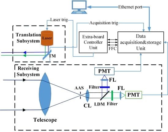
2. Instrument Configuration

A schematic diagram of the DWOL system is presented in Figure 1. This system consists of four components: a laser translation subsystem, a signal receiving subsystem, a data acquisition unit and a controller unit. The DWOL system maintains communication with the host computer, which can send control instructions to the DWOL system through an Ethernet port and can display the sampling results of the detected returning signals in real time. The designed parameters of the system are listed in

Table 1. Parameters designed for the DWOL system.

	Transmitter
Wavelength	532 nm and 486 nm
Pulse energy	5.4 mJ (532 nm) and 2.7 mJ (486 nm)
Laser repetition rate	100 Hz
Pulse width	4 ns (532 nm) and 8.7 ns (486 nm)
Beam divergence	2.4 mRad (532 nm) and 4.7 mRad (486 nm)
	Receiver
Telescope diameter	200 mm
Maximal field of view	25 mRad
Diameter of FOV spot size at the water surface	50–75 m
Optical efficiency	0.6
Detector	PMT
Detector efficiency	0.10
Sampling time resolution	1 ns
Plane height	2000–3000 m
Plane speed	200 km/h

, and details of the subsystems are provided in the following sections.

2.1. Transmitter Subsystem

The transmitter subsystem consists of a dual-wavelength laser of 486 nm and 532 nm and a transmitting mirror (TM). The dual-wavelength laser transmits 486 nm and 532 nm laser, simultaneously, rending the DWOL system compatible with both the open ocean water and coastal water detection. The TM in the transmitter subsystem is used to adjust the direction of the transmitting laser to ensure that the direction of the laser is parallel to the optical axis of the receiving telescope. This scheme provides the DWOL system with a higher receiving efficiency when returning signals are received from targets. The 486 nm and 532 nm laser beams are obtained by triple frequency and optical parametric oscillator (OPO) method. A schematic diagram of the system is shown in Figure 2 [28].

The overall technical route was designed as follows: First, two beams from 808 nm LD pumping sources are coupled into an optical oscillator via optical fibers to pump an Nd:YAG crystal at two ends in order to generate a 1064 nm seed pulse. The KD*P crystal acts as a Q-switch driven by a 100 Hz Q-switched signal. The 1064 nm seed pulse then enters the optical amplifier. The amplifier consists of a polarization beam splitter (PBS), an Nd:YAG crystal, a $\lambda /4$ plate and a total reflection mirror. The seed pulse is amplified in the optical amplifier with a side-pumped VCSEL to achieve two-way amplification. After amplification, the 1064 nm laser beam is shrunk by a condenser and then enters a doubled-frequency crystal, LBO1. After the light passes through the double-frequency crystal, the 532 nm laser is generated. The 532 nm laser beam is then outputted after a long-pass dichroic mirror (LDM). The remaining 1064 nm laser and part of 532 nm laser beam undergo a sum frequency process through an LBO2 crystal to generate a 355 nm laser beam. The 355 nm laser beam is used in the OPO cavity to generate a 486 nm laser beam through an OPO process. The OPO cavity consists of a high reflection mirror, an output coupler and two BBO crystals, which act as OPO crystals. After the OPO process, the 486 nm laser beam is generated. Ultimately, the 486 nm laser beam is combined with the 532 nm laser beam to be outputted.

2.2. Receiver Subsystem

In the receiver subsystem, the telescope receives the returning signals reflected by targets and then focuses them on the rear focal plane. An adjustable aperture stop (AAS) is set at the rear focal plane of the receiving telescope and is driven by a stepping motor. The size of the aperture stop can be adjusted according to the received signal, thus affecting the signal reception of the subsequent optical path. While passing through the AAS and the first collimating lens (CL), the returning signals are separated into a 486 nm laser component and a 532 nm laser component by an LDM. During this process, the 486 nm laser beam is reflected to the 486 nm receiving channel by the LDM, and the 532 nm laser beam is simultaneously reflected into the 532 nm receiving channel by the LDM. Finally, the 532 nm and 486 nm signals pass their respective filters and are focused by a focusing lens onto the photosensitive surfaces of the photomultiplier tube (PMT) detectors.

When the returning signal arrives at the photosensitive surface of the PMT, the PMT photocathode generates a series of photoelectrons, which are amplified after passing through several dynodes. Subsequently, when the photoelectrons arrive at the anode, the PMT detector outputs a corresponding current level, and after passing through the corresponding resistors in the following amplification circuit, the output current is then converted into a corresponding voltage value. The amplified voltage value is converted to a digitized value by a 10-bit analog-to-digital converter (ADC). For our DWOL system, the relationship between the analog value and the digitized value can be expressed as:

$$V_a=\frac{2.0V}{1024}{V}_d$$

(1)

Here, $V_a$ and $V_d$ represent the respective analog and digital values, and the value of 1024 is the maximum amplitude of the digitized value sampled by the ADC. The sampling rate of the acquisition board is 1 GHz; thus, the minimum time resolution of the DWOL system is one nanosecond.

3. Experiment Validation

The data used in this article were obtained from airborne and in situ shipborne experiment results. The experiments were conducted in the South China Sea, as shown in Figure 3. The sites C1, C2, G1, G2, G3 and B3 were the selected in situ sites near the flight track.

Digital topographic data were obtained from the ETOPO1 Global Relief Model published by the National Geophysical Data Center (NGDC) [29]. As shown in Figure 3a, the water depth in detection area exceeds 150 m. The airborne experiment was conducted from 7:30 p.m. to 9:30 p.m. (UTC+8) on the evening of 1 June 2019, to reduce the influence of background noise. Due to limitations in conducting the experiment, the shipborne experiment was performed from 10:00 a.m. to 2:00 p.m. (UTC+8) on 28 May 2019. Because the airborne and shipborne experiments were performed on different dates, some differences may arise between the shipborne and airborne results.

The processing of the airborne data will be divided into the following parts:

Step 1: The digitized values sampled by the acquisition card will be converted to the corresponding sampled photons;

Step 2: For each receiving channel of our DWOL system, the baseline values of the detectors are different and are varying with the acquisition time. To obtain the corresponding photon number, the baseline values will be corrected;

Step 3: As mentioned in the Introduction part, the PMT detectors will generate a series of APC photons after receiving a strong returning signal. In this step, we will design methods and instruments to correct the APC photons;

Step 4: The dark count photons of the detectors and the background photons are calculated as the total dark count (TDC) photons, then the actual received photons can be obtained by removing the APC photons and the TDC photons.

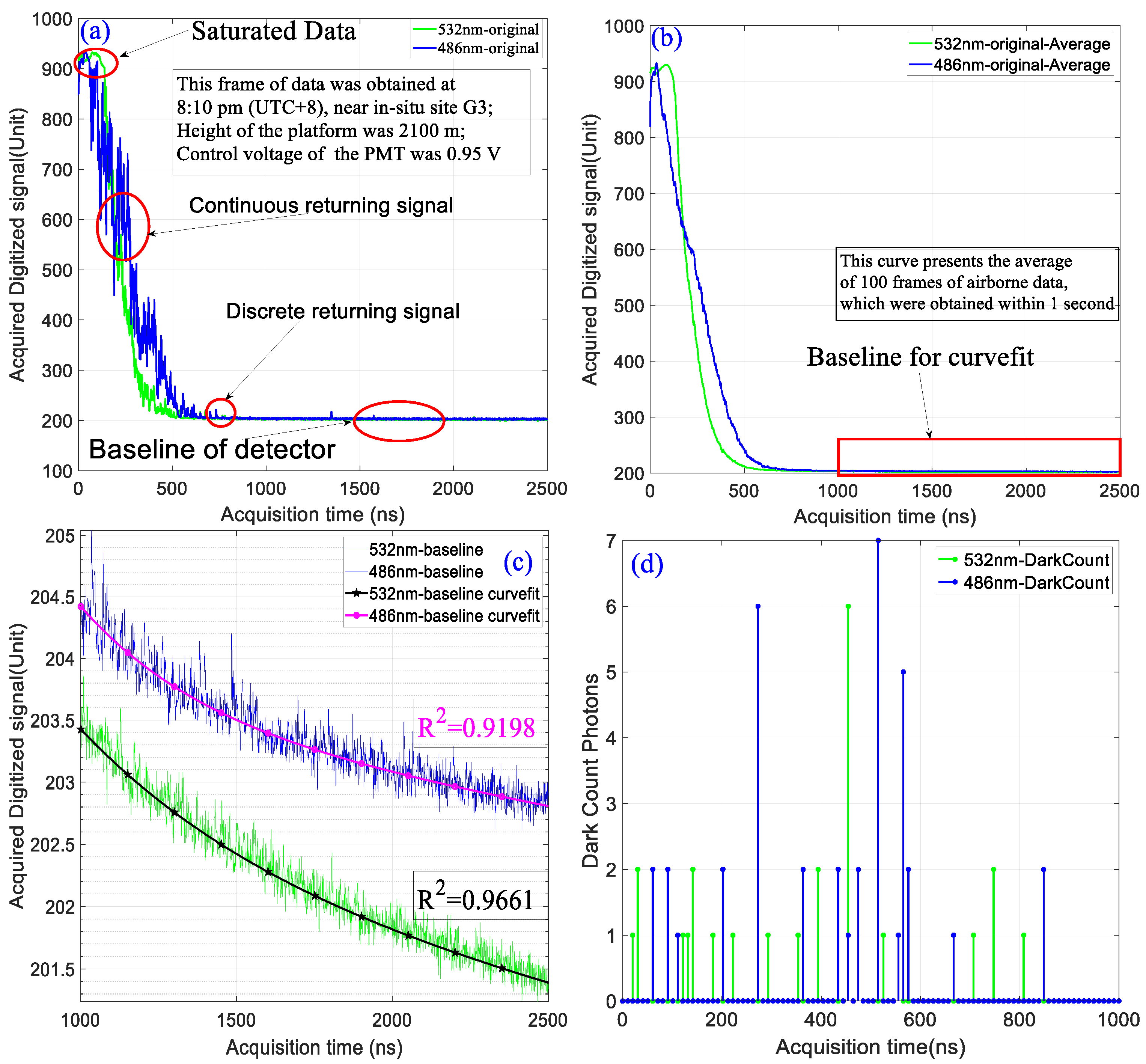
3.1. Conversion from the Sampled Digitized Voltage Values to the Corresponding Photon Number

According to Equation (1) the voltage values that output from the PMT detectors were converted to the digitized values by the ADC. One frame of the digitized signal is shown in Figure 4a. This frame of data contains the continuous returning signals scattered from the upper ocean water column and the discrete returning signals scattered from the deep water column. These signals will be converted to the corresponding photon number according to Equation (2), and the depth of the corresponding water column is described as Equation (3).

$$N=\frac{V-V_{baseline}}{V_{unit}}$$

(2)

$$L=\frac{\Delta t\ast c}{2n}$$

(3)

Here N is the number of acquired photons V is the digitized value of signal acquired by the ADC, the $V_{baseline}$ is the baseline value of the detector system shown in Figure 4a; and $V_{unit}$ is the response value for a single photon acquired via 532 nm or 486 nm laser channels. According to the PMT datasheet provided by the manufacturer, the $V_{unit}$ value for 532 and 486 nm channels is 8 for a control voltage of 0.95-V $L$ is the depth of the corresponding water column that backscatters the received photons, and $\Delta t$ is the flight time from the water surface to the corresponding water column, including back and forth motion. $c$ is the speed of light in vacuum, and $n$ is the refractive index of seawater.

As shown in Figure 4c, the $V_{baseline}$ value decreases following the form for a sum of two exponential functions of acquisition time, after a strong signal is received. To obtain a fitting function for the baseline value, we averaged 100 frames of data and performed a curve fitting about the acquisition time and the baseline value, as shown in Figure 4c. According to the curve-fitting results, the relationships for the 532 and 486 nm values are as follows:

$$\{\begin{array}{l}{y}_{486}=12.41e^{-0.002549(x-1000)}+203.9e^{-0.000002(x-1000)}\\ y_{532}=6.58e^{-0.00162(x-1000)}+202.7e^{-0.000003(x-1000)}\end{array}$$

(4)

Here, $x$ and $y$ represent the acquisition time and the baseline value, respectively.

This airborne experiment was conducted from 7:30 p.m. to 9:30 p.m. (UTC+8) on 1 June 2019; thus, the background noise received by the DWOL was quite low. For simplicity, in this study, the sum of the background noise and the dark count of the detector are denoted as the total dark count rate (TDCR). For the DWOL system, the number of acquired photons in bin i can be written as:

$$N(i)=N_{apc}(i)+N_r(i)+N_{tdc}(i)$$

(5)

where, $N(i)$ is the number of output photons converted from the response value sampled by the acquisition card, $N_{apc}(i)$ is the number of APC photons generated by the detector, $N_r(i)$ is the signal photons scattered from water column and $N_{tdc}(i)$ is the total number of dark count photons, shown in Figure 4d.

To evaluate the TDCR of the DWOL system, we recorded TDCR data for 22 s without the laser, as shown in Figure 4d. The results were converted from voltage signals to the corresponding photon number according to Equation (2).

The TDCR received by the DWOL system during one gating-time period can be calculated with Equation (6):

$$N_{TDCR}=\frac{N_{Total}}{\tau \ast n_{pulse}}$$

(6)

where, $N_{TDCR}$ is the number of TDCR photons acquired by the DWOL during one gating-time period, $\tau$ is the recording time, $n_{pulse}$ is the total number of laser pulses during the recording time and is the total number of noise photons received by the DWOL system during the recording time. $N_{Total}$ for 532 and 486 nm channel was 27 and 38, according to Equation (6), and the TDCR of the DWOL system for the 532 and 486 nm channels was 12.3 and 17.3 kHz per second, respectively. We applied 20 kHz for both channels to maximize the TDCR. According to this result, the average number of received noise photons in one gating-time period was 2e-5.

3.2. APC Correction

To eliminate the influence of the APC effect, we designed an APC calibration system (APCCS) to measure the APC occurrence probability distribution for input signal pulses of varying intensity, as shown in Figure 5.

Using the APCCS, the distributions of APC photons for the detectors were measured and the results are shown as follows in Figure 6:

The different attenuation from 0 dB to −40 dB shown in Figure 6 are obtained via the digital variable attenuator shown in Figure 5. From the results shown in Figure 6, we can see that when the intensity of the received signal is lower than −30 dB, the APC effect becomes negligible. In these results, the 0 dB results correspond to the APC effects generated by the returning signal from the water surface shown in Figure 4a. With the distribution of APC measured via the APCCS, the APC photons contained in bin i can be revised.

The APC photons in bin i are the integrated result obtained from bin 1 to bin i − 1, expressed as:

$$N_{apc}(i)={\displaystyle \sum _{j=1}^{i-1}{N}_{apc}(j;i)}$$

(7)

Here, j = 1, 2, 3, 4, …, i − 1, $N_{apc}(j;i)$ is the number of APC photons in bin i that were generated by the input pulse in the previous bin j. The APC photons number in bin i can be predicted by Equation (8).

$$N_{apc}(j;i)=N_{napc}(j)\ast P(j;i)=N_{napc}(j)\ast P(i-j)$$

(8)

where, $N_{napc}(j)$ is the number of APC photons in bin j, corrected for APC photons and $P(j;i)$ is the probability of detecting APC photons, measured using the APCCS shown in Figure 5. We assume that an APC photon cannot generate a subsequent APC photon; thus, the APC photons can be calculated with Equation (9):

$$N_{apc}(i)={\displaystyle \sum _{j=1}^{i-1}{N}_{napc}(j)\ast P(i-j)}$$

(9)

As shown in Figure 4a, the acquired signal was saturated due to strong reflection from the water surface. Moreover, the APC photons caused by the saturated data are not precisely predicted if the actual number of received photons in the saturated area is unknown. For this case, we proposed a new non-saturated value reference (NSVR) method to obtain the weight of saturated photons from the saturation area relative to a reference depth. A diagram of NSVR method is presented in Figure 7a.

The non-saturated data can be obtained when the airplane crosses a cloud and the incident laser intensity is attenuated. In this case, the acquired data for the DWOL are not saturated and thus can be taken as non-saturated data, as shown in Figure 7c. It is assumed that the water parameters remain constant from the surface to a depth of 20 m throughout the detection area; consequently, the returning photons from the detection water column can be described as:

$$\frac{N_i}{N_{ref}}=\frac{N{{}^{\prime }}_i}{N{{}^{\prime }}_{ref}}$$

(10)

Here, $N_{ref}$ and $N{{}^{\prime }}_{ref}$ are the number of saturated photons and non-saturated photons scattered from the corresponding reference depth, respectively. $N_i$ and $N{{}^{\prime }}_i$ are the number of acquired saturated photons and non-saturated in bin i. We captured several hundred frames of non-saturated data from three different sites, as shown in Figure 7b.

The relationship between the returning signals from bin i and the reference bin can be written as:

$$W=\frac{N_i}{N_{ref}}$$

(11)

here $W$ is the weight value of the acquired signal from bin i relative to the acquired signal from the reference depth. The weight of the signal from the water surface to that for the reference depth for the 532- and 486 nm channels is shown in Figure 8a,b. The figures demonstrate good consistency among the changing tendency of weights from different sites, indicating that the NSVR method is accurate. With NSVR method, the saturated returning photons scattered from water volume profiles can be calculated.

Additionally—to measure the APC with the APCCS—the attenuation of returning signals as a function of water depth should be calculated. The attenuation ratio from the water surface to a detecting depth can be described as:

$$AR=10\log (\frac{N_i}{N_{surf}})$$

(12)

Here, $AR$ is the attenuation ratio in dB, and $N_{surf}$ is the number of acquired returning photons from the water surface. Base on Equation (12), the attention values (in dB) from the water surface to the reference depth for the 532 and 486 nm channels are shown in Figure 8c,d.

In this study, the reference depths for the 486 and 532 nm channels are 10 and 15 m, respectively, as is shown in Figure 9.

As shown in Figure 9, the acquired returning signal from the reference depth is approximately 600 (unit) for 532 nm channel and approximately 700 (unit) for 486 nm channel. For simplicity, we take 650 (unit) as the reference value for both the 532 and 486 nm channels and according to Figure 8, the APC distribution from the saturated region can then be measured by APCCS.

Generally, we can divide the process of airborne data into six steps, the diagram of the process of airborne data is shown in Figure 10.

Step I: As shown in Figure 4b, the sampled values after the returning signals are obtained for the curving-fitting to obtain the function of the detector baseline, the function is described as Equation (4).

Step II: Using Equations (2) and (4), we converted the sampled digitized lidar signal in each bin i to the corresponding sampled photon number N(i), which is contained with dark count photons $N_{tdc}(i)$ and the after-pulse count photons $N_{apc}(i)$.

Step III: As shown in Figure 4d, we recorded the total dark count photons for each channel, the TDCR is calculated with Equation (6).

Step IV: Using the NSVR method and Equations (10) and (12), we recovered the corresponding received photons for the saturated data, the weight of the recovered saturated data to the reference data is shown in Figure 8. With this result and the APCCS, we obtained the APC distribution for different values of returning signals, shown in Figure 6. With the APC distribution result, we obtained the APC distribution functions.

Step V: With the APC distribution functions, we obtained the corresponding APC photons of $N_{apc}(i)$ for every sampled photons number $N(i)$.

Step VI: With Equation (5), we obtained the actual received photons in each bin i of $N_r(i)$.

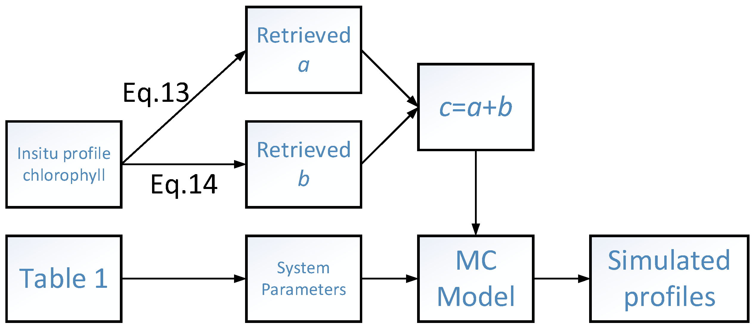
3.3. Monte Carlo Model Based on In Situ Shipborne Data

The in situ shipborne experiment was conducted near the flight track, as shown in Figure 3. To compare the shipborne and the airborne experiment results, a Monte Carlo (MC) model [30] was developed based on the shipborne experiment results.

The chlorophyll concentration results measured in the shipborne experiment are shown in Figure 11, which displays the measured results for G1, G2, B2 and C2, as C1 was near the turning area and G3 was far from the detecting area.

The results show that due to the limitations of instrument and experimental conditions, the deepest profiles of in situ chlorophyll concentration reached to 76 m; thus, the concentration profile beyond 76 m will be set equal to the concentration at 76 m.

The absorption coefficient a and scattering coefficient b are required for the MC model. In the shipborne experiment, the concentration of chlorophyll-a was obtained with RBR XR-420, which is designed by RBR, Ltd. in Canada. The absorption coefficient a and scattering coefficient b are obtained from Equations (13) and (14) [31,32]:

$$\{\begin{array}{l}a(\lambda )=a_w(\lambda )+a_{\varphi }(\lambda )+a_g(\lambda )\\ a_{\varphi }(\lambda )=\{a_0(\lambda )+a_1(\lambda )\ln [a_{\varphi }(440)]\}{a}_{\varphi }(440)\\ a_{\varphi }(440)=0.06{[Chl\_a]}^{0.65}\end{array}$$

(13)

and:

$$\{\begin{array}{l}b(\lambda )=b_w(\lambda )+b_p(\lambda )\\ b_p(\lambda )=B{[Chl\_a]}^{0.62}550/\lambda \end{array}$$

(14)

Here, $a(\lambda )$ is the total absorption coefficient, expressed as the sum of the absorption coefficients for pure water $a_w(\lambda )$, phytoplankton pigments $a_{\varphi }(\lambda )$ and yellow substance (YS) $a_g(\lambda )$ The absorption coefficient $a_w(\lambda )$ was obtained from Pope and Fry [33]. Considering that the airborne and shipborne experiments were conducted far from the mainland, the effect of YS was insignificant. The total scattering coefficient $b(\lambda )$ is expressed as the sum of the scattering coefficients for pure seawater $b_w(\lambda )$ and particles $b_p(\lambda )$ The scattering coefficients for pure seawater was taken from Morel [34], and the parameter B is an empirical value, set to 0.3 in this work [31]. The system parameters taken for MC model come from Table 1. The diagram of MC model is shown in Figure 12.

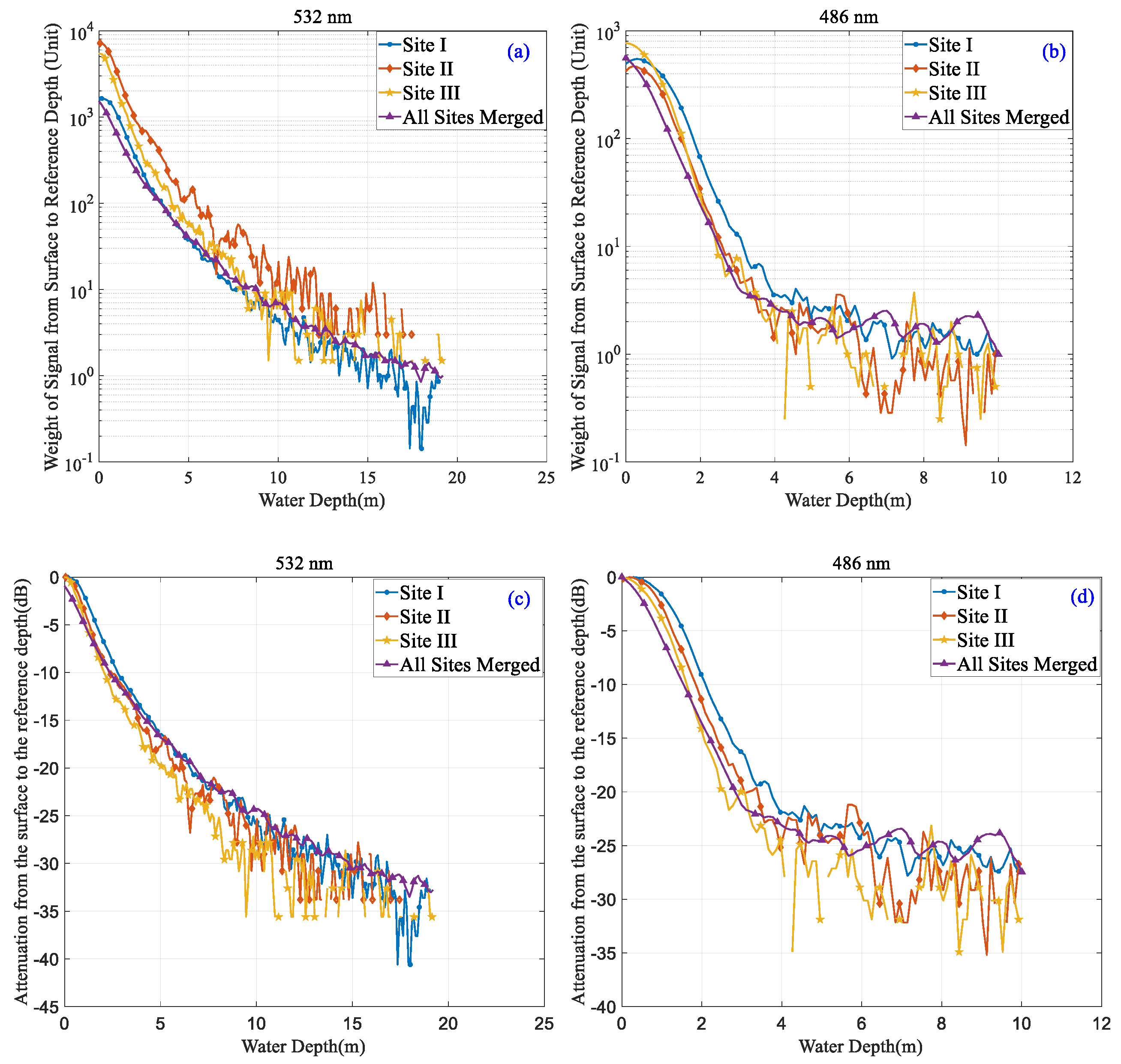
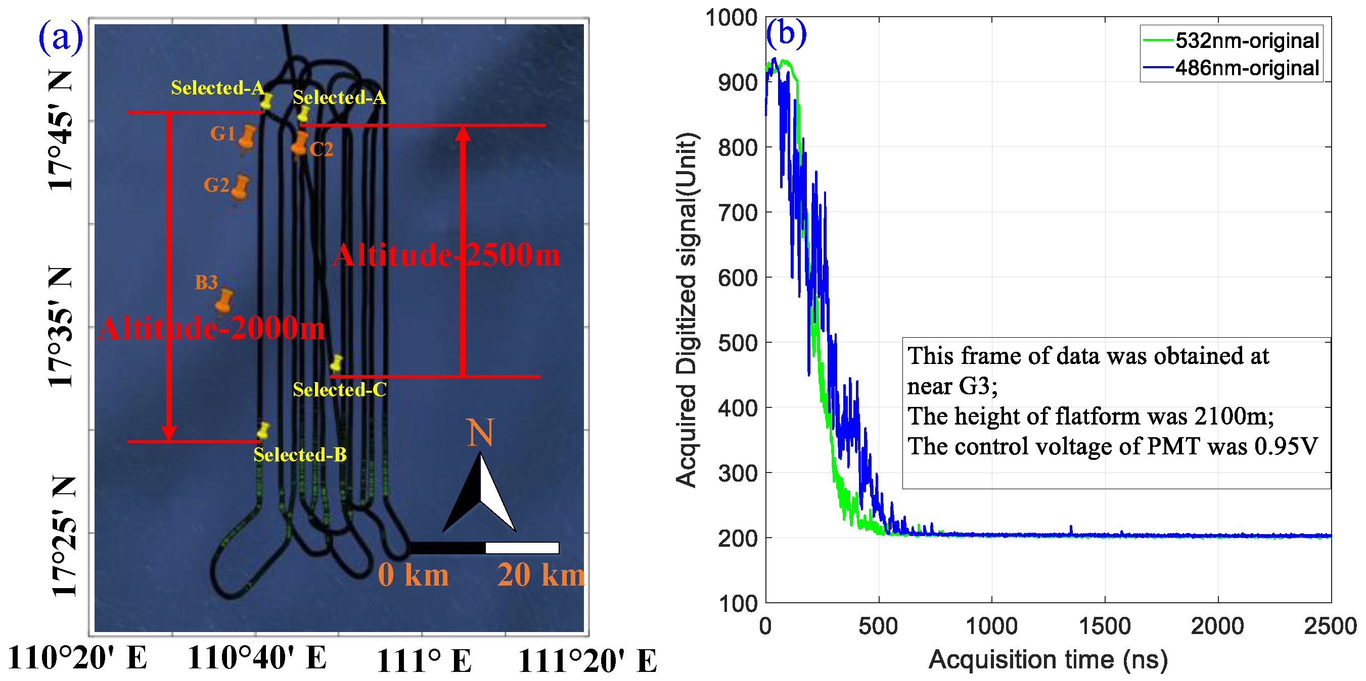
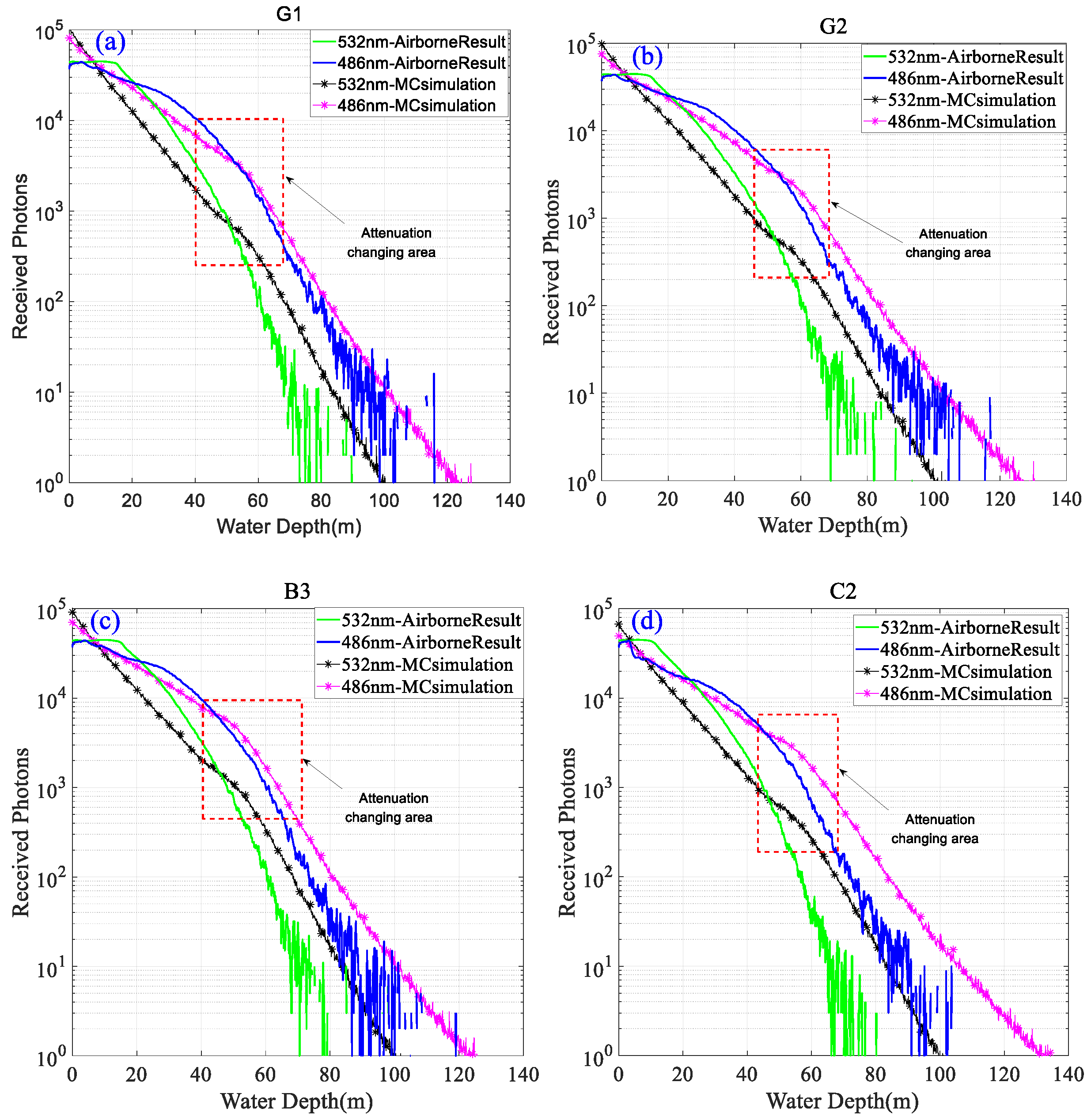
3.4. Airborne Experiment Results and Comparison with MC Simulation Results

To compare the airborne DWOL results and the in situ shipborne experiment results, we selected two datasets acquired near the shipborne in situ experiment sites. The flight track positions corresponding to these data are shown in Figure 13a. From Selected-A to Selected-B, height of the flying platform remained 2000 m, while from Selected-C to Selected-D, height of the flying platform remained 2500 m. One frame of selected data is shown in Figure 13b.

Considering that the laser repetition rate is 100 Hz, and the flight speed is approximately 50 m/s, we accumulated 500 frames of original data into a single frame to expand the dynamic range of the result. These 500 frames of data were obtained within 5 s. The accumulated results are shown in Figure 14a, where the X- and Y-axis values were converted to the water depth and the corresponding number of received photons, according to Equations (1) and (2).

As shown in Figure 14a, the received photons were mixed with the pseudo-photons generated by the after-pulse effect of the previously received photons. Following the calibration algorithm illustrated in Figure 10, the received photons were revised, as shown in Figure 14b. This figure shows that the APC photons primarily affect the results beyond 80 m for 486 nm channel and beyond 60 m for 532 nm channel. The revised water column profiles reached approximately 100 and approximately 80 m for 486 and 532 nm channels, respectively.

Using the Monte Carlo method, simulation results were obtained and compared with the airborne results, as shown in Figure 15.

The results show that the attenuation trend and the attenuation changing area of the airborne and the simulation results are highly consistent near in situ sites of G1, G2 and B3. The difference between the airborne results and simulation results may be caused by the different times of the shipborne and the airborne experiments, the errors in the absorption coefficient a and the scattering coefficient b converted with the bio-optical equation, calibration errors in the efficiency of the DWOL system, and the fatigue effect of the PMT detectors after a strong signal pulse. The difference appears to be larger at C2 because the chlorophyll concentration measured by the shipborne experiment was lower at that time; thus, the different dates may be responsible for the chlorophyll concentration difference in the airborne experiment.

4. Discussion

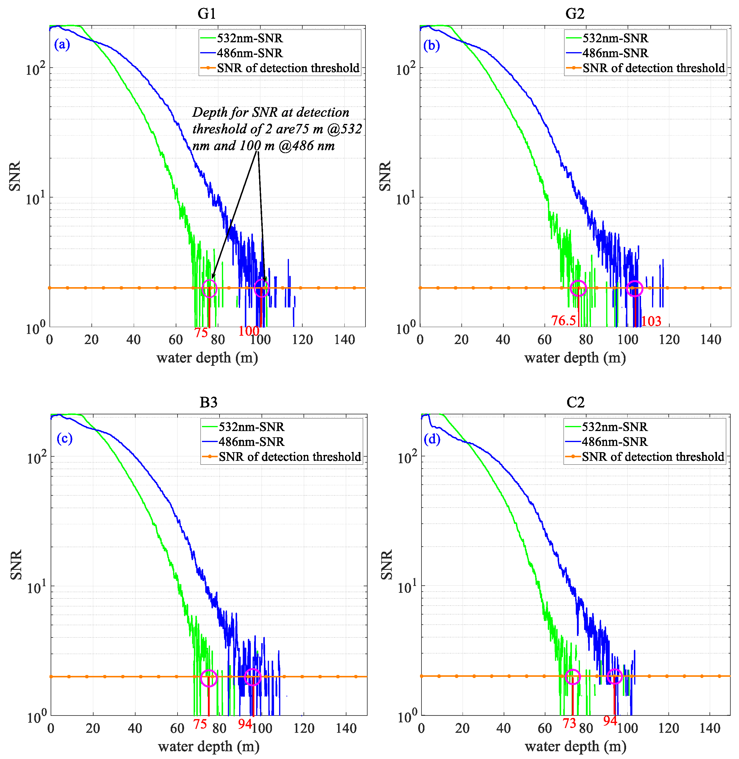
4.1. Signal-to-Noise Ratio

The signal-to-noise ratio (SNR) of the airborne experiment results is taken as a criterion to estimate the effectiveness of the airborne experiment results. The value of SNR is defined as:

$$SNR=\frac{N_s}{\sqrt{N_s+N_d+N_b}}$$

(15)

where $N_s$ is the received signal photons count, $N_d$ is the dark count photons acquired by the ADC and $N_b$ is the background photons. According to Equation (15), the values of SNR for 486 and 532 nm channels at G1, G2, B3 and C2 are shown in Figure 16.

Considering that it was hard for the DWOL system to distinguish between noise and signal photons if the SNR value was less than two, we take SNR of two as the criterion for the deepest vertical profiles. With this criterion, we concluded that the deepest vertical profiles for 532 nm channel reached to a depth of 75 m; while for 486 nm channel the deepest vertical profiles were extended to a depth of 100 m.

4.2. Inversion and Analysis of Water Column Parameters

To further analyze the rationality of the detection results, we inverted the lidar attenuation coefficients for 486 and 532 nm channels. In the detection area, the oceanic lidar equation can be written as [35]:

$$S(z)=K\frac{\beta (\pi ,z)}{{(nH+z)}^2}\exp [-2{\displaystyle {\int }_0^z\alpha (z{}^{\prime })}dz{}^{\prime }]$$

(16)

where K is a constant for the DWOL, $\beta (\pi ,z)$ is the volume scattering coefficient at a scattering angle of $\pi$ radians, $\alpha$ is the lidar attenuation coefficient, and H is the distance from the lidar to the water surface. Assuming that the water volume is homogeneous, the lidar equation can be rewritten in the following form:

$$\frac{d\{\ln [\frac{S{(nH+z)}^2}{K}]\}}{dz}=\frac{1}{\beta }\frac{d\beta }{dz}-2\alpha$$

(17)

If the water volume is homogeneous, then $d\beta /dz=0$; thus, Equation (17) can be rewritten as:

$$\alpha (z)=-\frac{d[\ln (S{}^{\prime })]}{2dz}$$

(18)

where $S{}^{\prime }=S{(nH+z)}^2$ is the range-corrected returning signal. We can then use the slope method (SM) to invert the lidar attenuation coefficient with Equation (18). The SM is applied here to compare the detection performance of the 486 and 532 nm channels with the same accuracy. If the operating depth of $dz$ is too small and the scattering coefficient of $\beta (z)$ is varying with depth, the SM will lose accuracy for the inversion results. To reduce the influence of $d\beta (z)/dz\ne 0$ and enhance the stability of signals returning from deeper water, the signal S’ was smoothed by applying a moving average method with a 41-ns span and the inverse results for $\alpha (z)$ were smoothed by using the Savity–Golay method [36], a filtering method based on local polynomial least squares fitting in time domain, with a 51-ns span. The inverted results are shown in Figure 17.

Considering that it is impossible for the lidar attenuation $\alpha (z)$ to be lower than the absorption coefficient of pure water; thus, we take the pure water absorption coefficient for 532- and 486 nm laser [33] as the criterion of the effectiveness for their corresponding inversion results, respectively. The results are shown in Figure 17. Figure 17a shows that, the effectiveness of ${\alpha }_{532}(z)$ reached near a depth of 75 m; while, the effectiveness of ${\alpha }_{486}(z)$ extended to a depth of approximately 93.m, which was about 24% deeper than that of 532 nm channel. From Figure 17, we can see that the effectiveness of profiles of ${\alpha }_{532}(z)$ was not deeper than 80 m. By contrast, the effectiveness of profiles for ${\alpha }_{486}(z)$ reached a depth of approximately 100 m. Moreover, the values of ${\alpha }_{486}(z)$ tended to be smaller after a depth of 80 m, indicating that the chlorophyll concentration became less beyond 80 m, which was in agreement with the shipborne results.

To illustrate the spatial change of lidar attenuation distribution along the flight track, we inverted the airborne data from Selected-A to Selected-B and Selected-C to Selected-D, as shown in Figure 13. The inverted results are shown in Figure 18.

The three-dimensional vertical profile distribution of ${\alpha }_{532}(z)$ and ${\alpha }_{486}(z)$ over the flight track are shown in Figure 19.

As shown in Figure 18 and Figure 19, the peak values of $\alpha (z)$ are primarily distributed between 60 m and 75 m, which is consistent with the shipborne experiment results shown in Figure 11. Figure 19 shows that the distribution of $\alpha (z)$ in the South China Sea is fairly stable, indicating that the CSL is mainly distributed from a depth of 40 to 80 m. Meanwhile, the distribution of ${\alpha }_{486}(z)$ extends to depth beyond 95 m, indicating that the 486 nm laser beam can potentially penetrate the entire CSL.

5. Conclusions

Airborne and shipborne experiments were conducted in a region of the South China Sea to evaluate the performance of the DWOL system. For a 500 frames accumulation, the experiments show that the DWOL system with a newly selected laser wavelength can detect water column profiles to approximately 100 m with the 486 nm channel operating from 2000 m. This depth is approximately 33% greater than that obtained by the 532 nm channel. The single-pulse energy of the 486 nm laser was 2.7 mJ, corresponding to one half of the energy for the 532 nm laser; however, even with a higher single-pulse energy, the deepest water column profiles detected with the 532 nm channel was only approximately 75 m.

The inverted results of the lidar attenuation coefficient $\alpha (z)$ showed that, the peak values of $\alpha (z)$ primarily ranged from 40 to 80 m. Additionally, the effectiveness of ${\alpha }_{532}(z)$ was no deeper than 80 m; however, the effectiveness of ${\alpha }_{486}(z)$ extended to approximately 100 m.

According to the comparison between the airborne and the shipborne experiment data and the inverted results of $a(z)$, we concluded that the vertical profiles obtained by the DWOL system reached a depth of 75 m for the 532 nm channel and 100 m for the 486 nm channel. Moreover, based on the inverted results the values of ${\alpha }_{486}(z)$ tended to decrease beyond 80 m, indicating that the 486 nm laser can potentially penetrate the entire CSL.

Future work will focus on the inversion of chlorophyll concentrations and other water parameters using data simultaneously obtained with 532- and 486 nm channels, for comparison with the results of shipborne experiments. This future work will focus on the advantages of multiple wavelengths for active ocean detection. In addition, the SBOL parameters based on the airborne results will be discussed. A new method for expanding the detection dynamics of DWOL system will also be investigated.

References

1. McClain, C.R. A decade of satellite ocean color observations. Annu. Rev. Mar. Sci. 2009, 1, 19–42. [Google Scholar] [CrossRef] [PubMed] [Green Version]
2. Siegel, D.A.; Behrenfeld, M.J.; Maritorena, S.; McClain, C.R.; Antoine, D.; Bailey, S.W.; Bontempi, P.S.; Boss, E.S.; Dierssen, H.M.; Doney, S.C. Regional to global assessments of phytoplankton dynamics from the SeaWiFS mission. Remote Sens. Environ. 2013, 135, 77–91. [Google Scholar] [CrossRef] [Green Version]
3. De Boyer Montégut, C.; Madec, G.; Fischer, A.S.; Lazar, A.; Iudicone, D. Mixed layer depth over the global ocean: An examination of profile data and a profile-based climatology. J. Geophys. Res. Oceans 2004, 109. [Google Scholar] [CrossRef]
4. Brainerd, K.E.; Gregg, M.C. Surface mixed and mixing layer depths. Deep Sea Res. Part I Oceanogr. Res. Pap. 1995, 42, 1521–1544. [Google Scholar] [CrossRef]
5. Morel, A.; Berthon, J.F. Surface pigments, algal biomass profiles, and potential production of the euphotic layer: Relationships reinvestigated in view of remote-sensing applications. Limnol. Oceanogr. 1989, 34, 1545–1562. [Google Scholar] [CrossRef] [Green Version]
6. Winker, D.M.; Vaughan, M.A.; Omar, A.; Hu, Y.; Powell, K.A.; Liu, Z.; Hunt, W.H.; Young, S.A. Overview of the CALIPSO mission and CALIOP data processing algorithms. J. Atmos. Ocean. Technol. 2009, 26, 2310–2323. [Google Scholar] [CrossRef]
7. Hu, Y. Ocean, Land and Meteorology Studies Using Space-Based Lidar Measurements; NASA Langley Research Center: Hampton, VA, USA, 2009.
8. Morel, A. Light and marine photosynthesis: A spectral model with geochemical and climatological implications. Prog. Oceanogr. 1991, 26, 263–306. [Google Scholar] [CrossRef]
9. Roesler, C.S.; Perry, M.J.; Carder, K.L. Modeling in situ phytoplankton absorption from total absorption spectra in productive inland marine waters. Limnol. Oceanogr. 1989, 34, 1510–1523. [Google Scholar] [CrossRef] [Green Version]
10. Bricaud, A.; Morel, A.; Prieur, L. Absorption by dissolved organic matter of the sea (yellow substance) in the UV and visible domains 1. Limnol. Oceanogr. 1981, 26, 43–53. [Google Scholar] [CrossRef]
11. Chen, S.; Xue, C.; Zhang, T.; Hu, L.; Chen, G.; Tang, J. Analysis of the Optimal Wavelength for Oceanographic Lidar at the Global Scale Based on the Inherent Optical Properties of Water. Remote Sens. 2019, 11, 2705. [Google Scholar] [CrossRef] [Green Version]
12. Wu, S.; Song, X.; Liu, B. Fraunhofer lidar prototype in the green spectral region for atmospheric boundary layer observations. Remote Sens. 2013, 5, 6079–6095. [Google Scholar] [CrossRef] [Green Version]
13. Kattawar, G.W.; Xu, X. Filling in of Fraunhofer lines in the ocean by Raman scattering. Appl. Opt. 1992, 31, 6491–6500. [Google Scholar] [CrossRef] [PubMed]
14. Chen, Z.; Fan, R.; Ye, G.; Luo, T.; Guan, J.; Zhou, Z.; Chen, D. Depth resolution improvement of streak tube imaging lidar system using three laser beams. Chin. Opt. Lett. 2018, 16, 041101. [Google Scholar] [CrossRef] [Green Version]
15. Gray, D.J.; Anderson, J.; Nelson, J.; Edwards, J. Using a multiwavelength LiDAR for improved remote sensing of natural waters. Appl. Opt. 2015, 54, F232–F242. [Google Scholar] [CrossRef]
16. Burton, S.; Ferrare, R.; Hostetler, C.; Hair, J.; Rogers, R.; Obland, M.; Butler, C.; Cook, A.; Harper, D.; Froyd, K. Aerosol classification using airborne High Spectral Resolution Lidar measurements-methodology and examples. Atmos. Meas. Tech. 2012, 5, 73. [Google Scholar] [CrossRef] [Green Version]
17. Sasano, Y.; Browell, E.V. Light scattering characteristics of various aerosol types derived from multiple wavelength lidar observations. Appl. Opt. 1989, 28, 1670–1679. [Google Scholar] [CrossRef]
18. Acharya, Y.; Sharma, S.; Chandra, H. Signal induced noise in PMT detection of lidar signals. Measurement 2004, 35, 269–276. [Google Scholar] [CrossRef]
19. Zhao, Y. Signal-induced fluorescence in photomultipliers in differential absorption lidar systems. Appl. Opt. 1999, 38, 4639–4648. [Google Scholar] [CrossRef]
20. Concannon, B.M.; Contarino, V.M.; Allocca, D.M.; Mullen, L.J. Characterization of signal-induced artifacts in photomultiplier tubes for underwater lidar applications. In Proceedings of Airborne and In-Water Underwater Imaging; SPIE: Denver, CO, USA, 1999; pp. 167–173. [Google Scholar]
21. Donovan, D.; Whiteway, J.; Carswell, A.I. Correction for nonlinear photon-counting effects in lidar systems. Appl. Opt. 1993, 32, 6742–6753. [Google Scholar] [CrossRef]
22. Lu, X.; Hu, Y.; Yang, Y.; Bontempi, P.; Omar, A.; Baize, R. Antarctic spring ice-edge blooms observed from space by ICESat-2. Remote Sens. Environ. 2020, 245, 111827. [Google Scholar] [CrossRef]
23. Yu, C.; Shangguan, M.; Xia, H.; Zhang, J.; Dou, X.; Pan, J.-W. Fully integrated free-running InGaAs/InP single-photon detector for accurate lidar applications. Opt. Express 2017, 25, 14611–14620. [Google Scholar] [CrossRef] [PubMed] [Green Version]
24. Lu, X.; Hu, Y.; Pelon, J.; Trepte, C.; Liu, K.; Rodier, S.; Zeng, S.; Lucker, P.; Verhappen, R.; Wilson, J. Retrieval of ocean subsurface particulate backscattering coefficient from space-borne CALIOP lidar measurements. Opt. Express 2016, 24, 29001–29008. [Google Scholar] [CrossRef] [PubMed]
25. Churnside, J.H.; McCarty, B.J.; Lu, X. Subsurface ocean signals from an orbiting polarization lidar. Remote Sens. 2013, 5, 3457–3475. [Google Scholar] [CrossRef] [Green Version]
26. Schutz, B.E.; Zwally, H.J.; Shuman, C.A.; Hancock, D.; DiMarzio, J.P. Overview of the ICESat mission. Geophys. Res. Lett. 2005, 32. [Google Scholar] [CrossRef] [Green Version]
27. Chen, G.; Tang, J.; Zhao, C.; Wu, S.; Yu, F.; Ma, C.; Xu, Y.; Chen, W.; Zhang, Y.; Liu, J. Concept Design of the “Guanlan” Science Mission: China’s Novel Contribution to Space Oceanography. Front. Mar. Sci. 2019, 6, 194. [Google Scholar] [CrossRef] [Green Version]
28. Ma, J.; Lu, T.; He, Y.; Jiang, Z.; Hou, C.; Li, K.; Liu, F.; Zhu, X.; Chen, W. Compact dual-wavelength blue-green laser for airborne ocean detection lidar. Appl. Opt. 2020, 59, C87–C91. [Google Scholar] [CrossRef]
29. Amante, C.; Eakins, B.W. ETOPO1 Arc-Minute Global Relief Model: Procedures, Data Sources and Analysis; 2009. Available online: http://www.ngdc.noaa.gov/mgg/global/global.html (accessed on 1 September 2020).
30. Wang, L.; Jacques, S.L.; Zheng, L. MCML—Monte Carlo modeling of light transport in multi-layered tissues. Comput. Methods Programs Biomed. 1995, 47, 131–146. [Google Scholar] [CrossRef]
31. Lee, Z.; Carder, K.L.; Mobley, C.D.; Steward, R.G.; Patch, J.S. Hyperspectral remote sensing for shallow waters. I. A semianalytical model. Appl. Opt. 1998, 37, 6329–6338. [Google Scholar] [CrossRef]
32. Morel, A. Optical modeling of the upper ocean in relation to its biogenous matter content (case I waters). J. Geophys. Res. Ocean 1988, 93, 10749–10768. [Google Scholar] [CrossRef] [Green Version]
33. Pope, R.M.; Fry, E.S. Absorption spectrum (380–700 nm) of pure water. II. Integrating cavity measurements. Appl. Opt. 1997, 36, 8710–8723. [Google Scholar] [CrossRef]
34. Morel, A. Optical properties of pure water and pure sea water. Opt. Asp. Oceanogr. 1974, 1, 1–24. [Google Scholar]
35. Churnside, J.H. Review of profiling oceanographic lidar. Opt. Eng. 2013, 53. [Google Scholar] [CrossRef] [Green Version]
36. SAVITZKY, A. Smoothing and Differentiation of Data by Simplified Least Squares Procedures. Anal. Chem. 1964, 36, 1627–1639. [Google Scholar] [CrossRef]
Figure 1. Schematic diagram of the dual-wavelength ocean lidar (DWOL) system. TM—transmitting mirror; AAS—adjustable aperture stop; CL—collimating lens; LDM—long-pass dichroic mirror; FL—focusing lens; PMT—photomultiplier tube; FFC—flexible flat cable.
Remotesensing 12 02844 g001
Figure 2. Schematic diagram of the 486 and 532 nm lasers.
Remotesensing 12 02844 g002
Figure 3. Experiments in the South China Sea. (a) Distributed flight track and selected in situ sites; (b) photograph of the DWOL system in airborne experiment.
Remotesensing 12 02844 g003
Figure 4. (a) Data for a single frame acquired by the acquisition board. Data obtained near in situ site G3, for a photomultiplier tube (PMT) control voltage of 0.95-V and a plane height of 2100 m; (b) average result for 100 frames of data acquired within 1 s near G3. Data acquired after 1000 ns were used as a curve-fit for the detector system baseline; (c) curve-fit results for the baselines of 532- and 486-nm channels. R-square values for 532- and 486 nm channels are 0.9661 and 0.9198, respectively; (d) dark count statistics for 532 and 486 nm channels, which were obtained without the laser.
Remotesensing 12 02844 g004
Figure 5. Diagram of the after-pulse count calibration system (APCCS).
Remotesensing 12 02844 g005
Figure 6. Distribution of the APC from attenuation of 0 to −40 dB. (a) attenuation of 0 dB; (b) attenuation of −5 dB; (c) attenuation of −10 dB; (d) attenuation of −15 dB; (e) attenuation of −20 dB; (f) attenuation of −25 dB; (g) attenuation of −30 dB; (h) attenuation of −35 dB; (i) attenuation of −40 dB.
Remotesensing 12 02844 g006
Figure 7. (a) Diagram of the non-saturated value reference (NSVR) method; (b) distribution of sites for capturing characteristic data; (c) non-saturated data for the 532- and 486 nm channels.
Remotesensing 12 02844 g007
Figure 8. (a) Change in weight with water depth for 532 nm, relative to the reference depth; (b) change in weight with water depth for 486 nm relative to the reference depth; (c) attenuation of weight from the surface to the reference depth for the 532 nm channel; (d) attenuation of weight from the surface to the reference depth for the 486 nm channel.
Remotesensing 12 02844 g008
Figure 9. Selection of reference depths for the 532 and 486 nm channels.
Remotesensing 12 02844 g009
Figure 10. Diagram of data process.
Remotesensing 12 02844 g010
Figure 11. Chlorophyll concentration at G1, G2, B3 and C2, measured in the shipborne experiment using the RBR XR-420. (a) chlorophyll concentration at G1; (b) chlorophyll concentration at G2; (c) chlorophyll concentration at B3; (d) chlorophyll concentration at C2.
Remotesensing 12 02844 g011
Figure 12. Diagram of in situ profile chlorophyll processing with Monte Carlo (MC) simulations.
Remotesensing 12 02844 g012
Figure 13. (a) Position of selected data; (b) one frame of data from the selected dataset.
Remotesensing 12 02844 g013
Figure 14. (a) Results of received photons for 500 accumulated frames without any corrections, (b) result of received photons, with the total dark count (TDC) and the after-pulse count (APC) removed; (c) comparison between the original results and the corrected results.
Remotesensing 12 02844 g014
Figure 15. (ac) Comparison between the simulation results and the airborne results at altitude of 2000 m; (d) comparison between the simulation results and the airborne results at altitude of 2500 m.
Remotesensing 12 02844 g015
Figure 16. Signal-to-noise ratio (SNR) of the receiving signal photons. (a) SNR of G1; (b) SNR of G2; (c) SNR of B3; (d) SNR of C2. The SNR threshold of detection for our DWOL system is 2. The corresponding depth indicated by the red lines were obtained based on the median values of depth when the SNR was lower than 2.
Remotesensing 12 02844 g016
Figure 17. Distribution of lidar attenuation α ( z ) from G1 to C2. (a) Distribution of lidar attenuation at G1; (b) Distribution of lidar attenuation at G2; (c) Distribution of lidar attenuation at B3; (d) Distribution of lidar attenuation at C2; To enhance the stability of the inverted results, the range-corrected returning signals S were smoothed by applying a moving average with a 41-ns span. The magenta curves were obtained by a secondary smoothing of the inverse results using the Savity–Golay method with a 51-ns span.
Remotesensing 12 02844 g017
Figure 18. (a) Distribution of α 532 ( z ) from Selected-A to Selected-B; (b) distribution of α 486 ( z ) from Selected-A to Selected-B; (c) distribution of α 532 ( z ) from Selected-C to Selected-D; (d) distribution of α 486 ( z ) from Selected-C to Selected-D.
Remotesensing 12 02844 g018
Figure 19. (a) Distribution of α 532 ( z ) from Selected-A to Selected-B; (b) distribution of from Selected-A to Selected-B; (c) distribution of α 532 ( z ) from Selected-C to Selected-D; (d) distribution of α 486 ( z ) from Selected-C to Selected-D. Value of α ( z ) limited from 0 to 0.2 for better visualization.
Remotesensing 12 02844 g019