Article

Tracking Rates of Forest Disturbance and Associated Carbon Loss in Areas of Illegal Amber Mining in Ukraine Using Landsat Time Series

1
Department of Forest Mensuration and Forest Management, National University of Life and Environmental Sciences of Ukraine, Heroiv Oborony Str. 15, 03041 Kyiv, Ukraine
2
Ecosystem Services and Management (ESM) Program, International Institute for Applied Systems Analysis, A-2361 Laxenburg, Austria
*
Author to whom correspondence should be addressed.
Remote Sens. 2020, 12(14), 2235; https://doi.org/10.3390/rs12142235
Submission received: 19 May 2020 / Revised: 24 June 2020 / Accepted: 9 July 2020 / Published: 12 July 2020
(This article belongs to the Special Issue Forest Biomass and Carbon Observation with Remote Sensing)

Abstract

:
Mapping forest disturbance is crucial for many applications related to decision-making for sustainable forest management. This study identified the effect of illegal amber mining on forest change and accumulated carbon stock across a study area of 8125.5 ha in northern Ukraine. Our method relies on the Google Earth Engine (GEE) implementation of the Landsat-based Detection of Trends in Disturbance and Recovery (LandTrendr) temporal segmentation algorithm of Landsat time-series (LTS) to derive yearly maps of forest disturbance and recovery in areas affected by amber extraction operations. We used virtual reality (VR) 360 interactive panoramic images taken from the sites to attribute four levels of forest disturbance associated with the delta normalized burn ratio (dNBR) and then calculated the carbon loss. We revealed that illegal amber extraction in Ukraine has been occurring since the middle of the 1990s, yielding 3260 ha of total disturbed area up to 2019. This study indicated that the area of forest disturbance increased dramatically during 2013–2014, and illegal amber operations persist. As a result, regrowth processes were mapped on only 375 ha of total disturbed area. The results were integrated into the Forest Stewardship Council® (FSC®) quality management system in the region to categorize Forest Management Units (FMUs) conforming to different disturbance rates and taking actions related to their certification status. Moreover, carbon loss evaluation allows the responsible forest management systems to be streamlined and to endorse ecosystem service assessment.

Graphical Abstract

1. Introduction

Mapping spatial and temporal patterns of forest disturbance is required for a broad range of applications that aim to understand the effect of forest structure change on ecosystem services. A reliable assessment of forest biomass dynamics is crucial for carbon cycle description, both globally [1,2] and at local scales [3]. In particular, an improved knowledge of aboveground biomass change will contribute to the more precise estimation of carbon dioxide emissions caused by deforestation [4]. Different types of forest disturbance affect the amount of live biomass removal and associated carbon storage. Thus, describing abrupt and long-lasting disturbance processes is important for reporting forest carbon fluxes [5]. In addition to major types of natural and human-induced disturbance (i.e., harvesting, wildfires, insect infestations, etc.), forests are often impacted by mining [6]. In particular, the forest structure in northern Ukraine has been altered by illegal amber mining [7,8]. Amber extraction operations have a dramatic impact on ecosystems, which damage the floral and soil components; however, the scale of the problem is still not clearly understood. Since there is a lack of reliable historical records of areas disturbed by amber mining, assessing their impact on ecosystem services over time has been limited.
Recently, major advances in tracking changes in forest structure have been made using the free, historically rich and well calibrated archive of Landsat imagery [9]. The availability of Earth observation data that have been captured for more than three decades by the Landsat Thematic Mapper (TM), Enhanced Thematic Mapper Plus (ETM+), and Operational Land Imager (OLI) sensors has altered forest change classification towards pixel-based approaches [10]. As a result of improvements in large data processing capacity, retrieving disturbance and recovery events from spectral trajectories have become a new standard for change detection [11,12]. Spectral segmentation coupled with machine learning algorithms have provided new opportunities to capture spectral profiles imposed by abrupt as well as gradual non-stand-replacing disturbance agents [13,14]. Similarly, the analysis of spectral trajectories has supported the detection of forest recovery processes [15]. Thus, the ability to depict specific change agents using Landsat time series (LTS) has proven to be useful for developing consistent forest biomass monitoring systems [16].
According to the literature review by Zhu [17], applications of LTS have increased substantially in recent years. Notable advancements in data processing have been made possible due to changes in the data distribution policy in 2008 [18]. Based on a multi-date archive of imagery, methods for global and national land cover characterization and change detection have been developed [19,20], which were previously applied only to satellite data with a coarser spatial resolution. Access to the large Landsat archive has shifted the data analysis paradigm in remote sensing [21,22]. A transition from scene-centered towards pixel-based image composite approaches [10] have allowed significant developments in temporal image composite methods without the need to search for cloud-free images. Roy et al. [19] proposed the maximum Normalized Difference Vegetation Index (NDVI) composite procedure, which preferentially selects the “greenest” pixels within a specific time domain (e.g., monthly, seasonal, and annual). Flood [23] developed a multi-temporal compositing approach based on medoids in spectral space over a time period that is robust to extreme values and unbiased in favor of images with denser green vegetation. Alternatively, White et al. [22] reported on an image composition technique that assigns scores to pixels based on sensor type, year, seasonality, and data quality, and then allows the best-available-pixels (BAP) to be selected for forest cover mapping over large territories.
Historically, forest disturbance was detected using remote sensing data for two distinct points in time. According to Hansen and Loveland [24], legacy bi-temporal change detection techniques were used in the past due to the high costs associated with processing imagery over multiple time periods and the poor data availability. Unlike single-date comparison, which indicates only whether change has occurred, time series algorithms are based on the mass-processing of satellite imagery, capable of detecting different types of disturbance [12,14]. Available approaches of forest disturbance mapping using LTS were classified in a literature review by Zhu [17] into six major groups (i.e., thresholding, differencing, segmentation, trajectory classification, statistical boundary, and regression). While most of the algorithms focus on abrupt changes to forest structure, temporal segmentation approaches, such as Landsat-based Detection of Trends in Disturbance and Recovery (LandTrendr) [11], provide information on the magnitude and rate of disturbance processes that leverage the detection of causal agents [25]. Given the temporally rich LTS, change patterns can be revealed as a function of time, describing both abrupt (i.e., harvest, wildfires, etc.) or long-lasting disturbance (i.e., thinning, insect-related mortality, etc.) and regrowth events. Potentially, the spectral profile of certain disturbances can be identified by predefined shape patterns of spectral matrices that reflect the known response of vegetation to shifts in environmental conditions [26]. Senf et al. [27] found that LTS are suitable for characterizing different change events, even though it is still difficult to automatically determine the exact disturbance onset, especially those with a long duration. Recent studies have evaluated ensemble techniques that fuse pixel-based time series analysis and raster classifiers to improve change detection and forest disturbance mapping [28,29].
Vegetation change monitoring using LTS has limitations because the algorithms are computationally expensive and require large volumes of data storage. The Google Earth Engine (GEE) cloud-based platform has emerged as a powerful solution to accelerate mass data processing [30]. Several temporal segmentation algorithms have already been implemented as a GEE application and programming interface (API) including the Continuous Change Detection and Classification (CCDC) [31], the Vegetation Change Tracker (VCT) [32], and LandTrendr [33]. The availability of radiometrically corrected imagery is another important advantage of a GEE cloud-based computational platform for tracking forest change using LTS. It provides access to surface reflectance Landsat images generated with the Landsat Ecosystem Disturbance Adaptive Processing System (LEDAPS) [34] and the Land Surface Reflectance Code (LaSRC) [35], which are considered to be the most robust atmospheric correction methods to date. Additionally, these datasets are delivered with cloud/shadow masks robustly detected by the CFMask algorithm [36], which are important for producing spatially continuous cloud-free composited mosaics. The GEE implementation of the LandTrendr algorithm has been increasingly examined for vegetation disturbance and recovery mapping within different temporal and spatial domains [37,38,39].
Forest disturbance and recovery mapping using optical remote sensing technologies is based on the properties of canopy structure changes that can be captured using different spectral indices. The short-wave infrared (SWIR) band is usually favored because of its sensitivity to vegetation moisture and canopy cover. In this regard, the normalized burn ratio (NBR) [40] is often used for forest disturbance detection. In addition to higher sensitivity to disturbance events in comparison with other indices, previous studies have proven that the delta NBR (dNBR) is useful for describing specific levels of disturbance and recovery [41]. For example, Bright et al. [37] analyzed post-fire vegetation recovery using LandTrendr-fitted spectral trajectories of NBR as an indicator variable for its conditions. The NBR and NDVI were found to be the most suitable for interannual vegetation changes in LTS analysis [42]. Similarly, Hislop et al. [43] demonstrated that both indices accurately capture wildfire disturbance in pixel-based approaches; however, it was shown that NDVI is not so reliable in southeast Australia for detecting post-fire recovery of sclerophyll forests. This is because the NDVI is sensitive to moisture content and canopy structure, indicating a return to pre-fire values within 3–5 years, while, for the NBR, this period is twice as long. Higher capacity for distinguishing different levels of forest recovery was also reported by Nguyen et al. [14]. Many studies [14,15,41,43] have been focused on various components of Tasseled-Cap (TC) transformation [44]. The potential for differentiating disturbances associated with some insect agents in the forest ecosystems of Canada have been revealed using TC wetness, greenness, and brightness components [45]. Ultimately, these indices contribute to the accurate classification of different types of disturbance using temporally normalized LTS [46].
While forest ecosystems are highly influenced by different disturbance processes, remote sensing has become of great interest in characterizing forest dynamics over space and time. LTS provide valuable information on the state and dynamics of forests and can enhance our knowledge of ecosystem services. Forest biomass is a key parameter for describing global biochemical processes that is extracted preferentially across space and time using LTS [9]. A review of the literature shows continuously improving techniques to track both natural and human-induced disturbances; however, studies focusing on forest damage caused by mining are still rare [6,39]. Nevertheless, illegal amber mining in Ukraine has been recognized as a major forest-destroying disturbance in Ukraine during the last decade, which has a direct influence on the carbon sink. The lack of spatially explicit information on mining processes complicates the calculation of forest biomass and carbon loss in areas disturbed by amber extraction. Although examples of published works exist that provide methods for accurate mapping of forest disturbance using LTS in this region, there are no quantitative assessments of the mining history.
Efforts to combat the infringement of applicable laws in forestry is a critical part of the current forest management of the country. During 2019, the volume of illegal logging in forests managed by the state forest management units (FMUs) increased by more than six-fold. Unauthorized or illegal resource use is also unacceptable in accordance with Forest Stewardship Council® (FSC®) standards [47]. A distinct advantage of using remote sensing tools is that it is possible to avoid mistakes of a human nature, reduce the costs of monitoring, and mitigate the risks related to the health and safety of the researchers and workers involved. The last point is very important, considering reports of threats to observers of illegal amber mining [7,8].
Our study has taken the advancement of freely available LTS and the LandTrendr image segmentation algorithm to be the first to reveal the actual scale of forest damage caused by illegal mining in northern Ukraine. The aim of this work was threefold: (1) to explore the capability of detecting different levels of forest disturbance in areas affected by mining operations using the NBR time series; (2) to evaluate ecosystem service losses, in particular carbon, associated with illegal amber operations; and (3) to introduce the methodology to the state forest monitoring system and FSC audit practices based on the scale and level of disturbance.

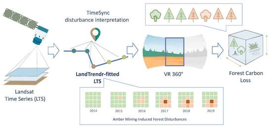
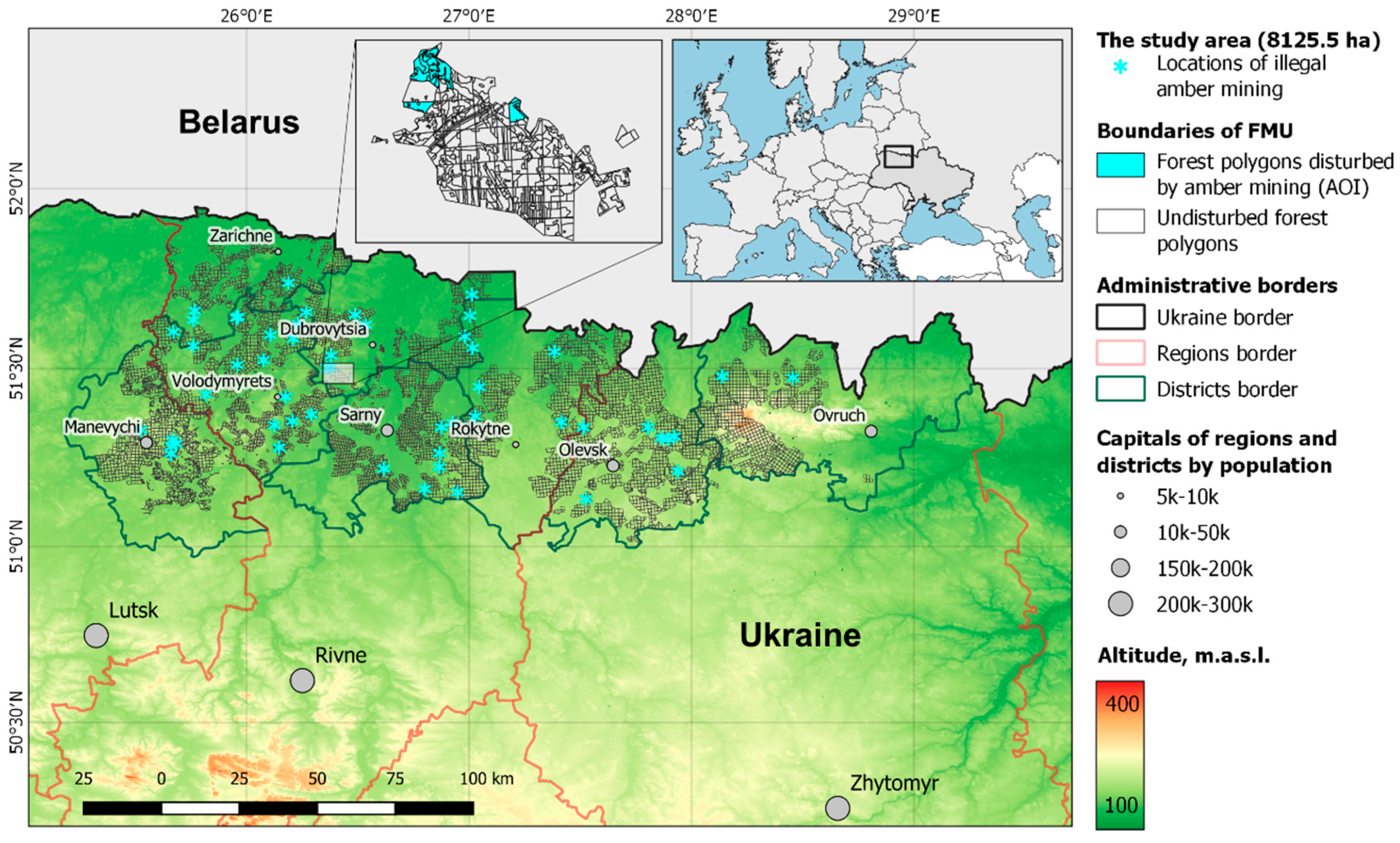
2. Materials and Methods
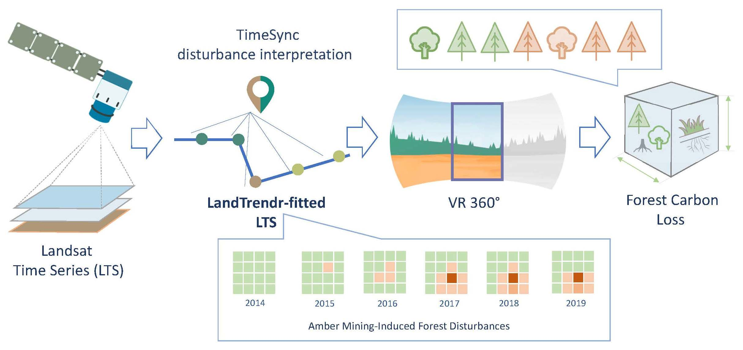
2.1. Study Area

The study area of 8125.5 ha is scattered along the Belarus border in the northernmost districts of the Zhytomyr, Rivne, and Volyn oblasts (regions). We used the State Forest Agency of Ukraine list of plots disturbed by illegal amber mining to delineate the area. In particular, the field survey conducted by the forest guards in 2018 revealed that 2017 forest polygons located in 52 sub-units of the FMUs (sub-FMUs) were subject to illegal amber mining. Thus, we specified 52 distinct areas of interest (AOI) that included all the forest polygons that were officially reported as disturbed to some extent due to amber extraction operations. Hereafter, we refer to them as the study area (Figure 1).
In addition, the study area is located within eight districts (i.e., Ovruch, Olevsk (Zhytomyr region), Rokytne, Sarny, Dubrovytsia, Volodymyrets, Zarichne (Rivne region), and Manevychi (Volyn region)), which belong to the Ukrainian Polissya climatic zone with relatively high (up to 35–40%) forest cover [48] and a preferentially flat topographic position.
The study area is dominated (75.5%) by forests (Table 1). Wetlands contribute 16.2% to the total area, followed by unforested areas (i.e., unstocked planted forests, harvested areas, dead forests, barrens, and glades) that occupy 6.4% of the area. The share of grasslands and other unproductive lands (i.e., sands, channels, and quarries) is negligible (about 2%). Approximately one half (3297.6 ha) of the forested area is occupied by Scots pine. Silver birch and black alder forests dominate in the area with 2042.4 ha, while the share of Common oak is only 666.0 ha. The rest of the forested area belongs to other tree species (e.g., aspen, willow, etc.).
From estimates, Ukraine has one of the largest deposits of amber in the world [7]. Mining there has been uncontrolled by the authorities so that amber mining has become established, most commonly using industrial water pumps [8]. Given the relatively small depth of the deposition (about 2–10 m), extracting amber using the hydraulic method is simple but extremely damaging to the environment. It consists of pumping water under pressure into the soil, which releases pieces of amber onto the surface. Due to the impact of the water, decomposed organic matter is mixed with other soil horizons, which is the leading cause of soil erosion. Uncontrolled amber mining causes huge environmental damage and has contributed to the vast degradation of forest stands. The effect of pumping by itself destroys the forest structure, which results in further forest decline. Some areas are initially cleared of woody vegetation to produce large areas for the mining operation. Places affected by mining operations usually have little chance of recovery unless they have just been surveyed using shovels.

2.2. Reference Data

2.2.1. Field Survey Data

Traditionally, forest resources in Ukraine are estimated using a stand-wise forest inventory. The field survey is carried out in typical places in relatively small (i.e., 0.3–10 ha) and homogeneous (in terms of tree species, age, mean diameter, mean height, basal area, etc.) compartments using instruments to measure the stand parameters. The attribute information is coupled with forest polygon coverages and stored in georeferenced databases. Both the forest attribute data and the stand boundaries are continuously updated in response to any changes caused by harvests, wildfires, sylvicultural treatments, or other forest disturbances that have occurred within the 10-year revision period. Forest attributes, such as growing stock volume, are updated by means of growth models. An inventory by compartment with a continuous updating approach delivers the necessary data for forest management purposes for the forthcoming planning decade [49] but has been considered in this study as only one of the available sources of forest inventory information. For each forest polygon, we extracted information regarding land cover, tree species, age, growing stock, etc., from the forest inventory database of the Ukrainian Government Project Association (PA “Ukrderzhlisproekt”) and used these data for carbon loss estimation.

2.2.2. TimeSync Reference Data

A reference dataset characterizing forest polygons disturbed by amber mining was collected using the TimeSync interpretation tool [50], which was applied to 1554 Landsat one-pixel samples. We applied a 1% intensity sampling to each AOI. However, if the effect of mining in the AOI was too small, we adjusted the sample size such that it accounted for at least 20 pixels. Thus, it varied from 20 to 160 randomly sampled 30-m pixels within each AOI in the study area.
TimeSync v. 3.0 facilitated the visual interpretation of historical disturbance events using manual segmentation of LTS according to the reference data collection protocol [26,28,46]. The process of interpretation involved the analysis of sample points using a series of Landsat chips for 1984–2019 with the aid of freely available multi-date Google Earth (GE) images. The incorporation of finer-resolution GE images was crucial for properly assigning the land cover category and for distinguishing between stand replacement events caused by amber operations (marked as “mechanical”) from the structural changes (marked as “structural decline”) of the forest stands. The area was identified to be disturbed if a change in the NBR values between two vertices of a segment was greater than 100.
During interpretation, we discriminated amber mining from other types of disturbance that might potentially occur in the aforementioned time frame. Initially, we found that amber-related disturbances refer to the last decreasing trajectory of the NBR. In the case of amber mining, this trajectory might be characterized by different rates that result in more than one segment. Thus, among the data recorded for each sample point, we specified the onset year of disturbance. We found that, in most cases, illegal amber operations started after 2013–2014, but, in some cases, they date back to the middle of the 1990s. All changes in the forest structure that occurred before the onset year were attributed to other types of disturbance (marked in the TimeSync interpretation tool as “harvest”, “fire”, or “other”).
Collected through the TimeSync analysis, the data were then used as a reference for the accuracy assessment of the disturbance maps produced here. We also linked two types of forest disturbance associated with amber mining (i.e., stand replacement and structural decline) in the reference dataset to the four specified and mapped dNBR levels of disturbance with the aid of field validation.

2.2.3. Field Validation Data

The collection of field validation data was challenging because of the high risk to life and safety from the people involved in illegal amber extraction. Thus, a decision was made to minimize these risks through rapid picture-taking in easy-to-reach places within disturbed areas located in seven sub-FMUs of the Rivne region. To identify all levels of forest disturbance, the images were taken before the leaf-on period (April 2018) when it was possible to capture minor changes associated with the removal of the understory and to obtain more depth of field. The photos were subsequently transformed into virtual reality (VR) 360 interactive panoramic images and analyzed more closely [51,52,53]. We used a Nikon D5300 mirror digital camera equipped with a Nikon DX AF-S Nikkor 18–55 mm 1:3.5–5.6 G VR lens to take photos in manual mode. We applied an identical exposure and a 60% overlap to all photos. In total, around 3700 photos were taken in April 2018 at 69 sample locations, which were selected randomly from the TimeSync reference dataset.
Further steps in the data validation were completed though the interpretation of the spherical VR360 interactive panoramic images using a VR headset. The point at which the photos were taken was considered to be the center of a circular plot with a radius of 15 m. Given the 360-degree view of the sites, we interpreted the disturbances, thus creating an independent reference dataset that was used to evaluate the overall accuracy of the disturbance maps. Examples of some of the VR360 images are provided in the Supplementary Materials (Figures S1–S4).

2.2.4. Dataset for Biomass Estimation

Experimental data on the Scotch pine forest above-ground live biomass were collected at 17 temporary sample plots (TSPs) in the Ukrainian Polissya climatic zone. We also incorporated a dataset of 127 TSPs from a database containing estimates of live biomass from Ukrainian pine forests [54]. The TSPs were demarcated on-site in accordance with the relevant national requirements for forest inventory sample plots. The size of the TSP is defined based on the number of trees of the target species. Usually, they included at least 200–250 trees for middle-aged and mature stands and 350–500 for young stands; thus, the area of TSPs ranged from 0.05 to 1.50 ha. Diameter at breast height was measured for every tree (thicker than 2 cm). A total of 5–15 sample trees for each TSP was selected proportionally to the diameter class distribution. After the sample trees were felled, the main biometric tree parameters were measured, including stem length from stump to the top; the height of the stump; the length of the branch-free section of the stem; the stem height at which the first live branch is attached; the tree age; the five-year height increment of a tree; and the bark thickness and the five-year diameter increment at stump height, the breast height (1.3 m), and at the middle of the stem sections. The biomass of the branches and foliage were weighed separately. The stem, branches, and foliage biomass samples were further processed in a laboratory, aimed at investigating the density of the live above-ground biomass components.

2.2.5. Live Biomass Model

The biomass expansion factors for Scots pine were estimated using 144 sample plots collected in the Ukrainian Polissya. The models are presented in the following form:
R fr = M fr GS = a 0 + A a 1 × SI a 2 × RS a 3 × exp ( a 4 × A + a 5 × RS )
where Rfr is the biomass expansion factor; Mfr is the live biomass of fraction fr, oven-dry t ha−1; GS is the growing stock volume in m3; A is age in years; RS is relative stocking; SI is the site index, which reflects the quality of the site [55]; and a0–a5 are model parameters. Table 2 shows the parameters for the biomass of the stem, branches, and the foliage of pine forests and reports the coefficient of determination (R2).
The parameters of the forest live biomass for birch, black alder and aspen forests were taken from earlier studies conducted in the Ukrainian Polissya [56]. Furthermore, parameters for the oak and spruce total forest biomass and for tree roots, green forest floor (GFF), and the understory of the pine forests were taken from Shvidenko et al. [55].

2.3. Mapping Approach

2.3.1. LTS Pre-Processing and Segmentation

We used the GEE [30] implementation of the LandTrendr [33] algorithm to map forest disturbances and recovery rates in areas disturbed by amber mining. LandTrendr incorporates temporal segmentation and a fitting approach for each pixel of the LTS, originally developed by Kennedy et al. [11]. It identifies breakpoints (vertices) and determines straight-line trajectories that result in a new fitted-to-vertex (FTV) time series. The output is a new LTS for which the pixel values between vertices are interpolated using the line fit, consequently with reduced year-to-year noise. The performance of the algorithm is controlled by a set of parameters for customization. Depending on the time frame, the complexity of the disturbance history, and the spectral variation, long-lasting disturbance processes can be presented by either one or multiple spectral segments (Figure 2). The LandTrendr algorithm is recognized to be data intensive because it requires multiple access to the time series; thus, the parallel processing offered by the cloud-based GEE platform facilitates forest disturbance and regrowth mapping for large scale analysis [37,38] and was used in our study.
In this study, we used atmospherically corrected surface reflectance LTS that were generated using the LEDAPS [34] and LaSRC [35] algorithms applied to the Landsat TM, ETM+, and OLI sensors, respectively. Clouds and cloud shadows have been filtered using masks produced by the CFMask algorithm [36]. The images were filtered for the time domain of 1984–2019 to cover only the leaf-on period from 1 June to 31 August. To provide continuity in the LTS, we transformed the OLI data to match the ETM+ surface reflectance using the regression coefficients proposed by Roy et al. [57]. The harmonization procedure outlined here allows us to integrate the spectral data that are consistent in time and perform inter-sensor compositing of multiple observations into one summer observation per year. We used the medoid compositing procedure [23], which is robust and fast for the LandTrendr implementation, is not biased in favor of maximum values, and handles actual pixel values. Then, the NBR was calculated and used as an input for further temporal segmentation. The parameters of the LandTrendr algorithm were set based on prior works [37,46] that have shown them to perform adequately in terms of mapping forest disturbance and recovery. It is important to note that we adjusted the temporal segmentation procedure such that up to six segments can be fitted to the LTS.

2.3.2. Detecting Forest Disturbance and Recovery

Change detection in our study was based on the temporal segmentation of the NBR. LandTrendr can capture long-lasting and abrupt forest changes that are characterized by a set of metrics such as magnitude, rate, and duration. For each pixel, the disturbance events were defined as decreasing trajectories of NBR between two vertices. The recovery, in contrast, is considered as a trajectory showing a monotonic increase while stable trend segments represent undisturbed conditions. In addition to the temporal segmentation of NBR values, LandTrendr provides the vertex file storing the per-pixel segmentation information. First, for each AOI, we detected the onset year of disturbance using the TimeSync interpretation tool and produced pre-disturbance reference NBR mosaics. We performed per-pixel analysis of the vertex file to retain the last undisturbed NBR value following the onset year within the AOI as the candidate for the mosaic. Then, the FTV NBR time series were used to calculate yearly dNBR values up to 2019. To further perform the carbon loss calculations, we reclassified the continuous disturbance maps containing the dNBR values into discreate classes. Four common disturbance severity levels [40] determined through interpretation of the VR360 panoramic images were assigned as follows: low (dNBR = 100–269), moderate-low (dNBR = 270–439), moderate-high (dNBR = 440–659), and high (dNBR ≥ 660). The pixels with dNBR values lower than 100 were treated as undisturbed. The reclassification was introduced as an opportunity for distinguishing the severity levels associated with stand-replacing disturbances. Ultimately, the mapped yearly disturbance area was accumulated to report the total area of illegal amber mining in the AOI.
Post-disturbance regrowth was mapped using the last recovery segment from the vertex file if it was not followed subsequently by a disturbance segment. This analysis was performed within the cumulative disturbance footprint so that regrowth occurring outside of areas disturbed by amber mining were not included.

2.3.3. Map Accuracy Assessment

The accuracy of the mapped area was evaluated in two ways. First, we assessed the agreement between four disturbance levels as estimated using the dNBR and the magnitude of change process. The magnitude was identified using the TimeSync tool and reported as stand-replacing and non-stand-replacing disturbances. Secondly, we tested agreement between mapped dNBR severity levels and field observations using 69 VR360 panoramic images. It is also worth noting that the dNBR values were extracted from the disturbance maps for 2018 since it was important to match the year of the field data collection with the Landsat images. Ultimately, the results on the magnitude of forest change were addressed to accurately calculate the carbon loss.
The accuracy of the disturbance maps was assessed using the TimeSync validation dataset of 1554 sample points that were centered on 30 m × 30 m pixels. Because the data were collected through visual interpretation of LTS and GE images, we considered three map classes: undisturbed areas; non-stand-replacing disturbance (dNBR severity level equals 1); and stand-replacing disturbance (corresponds to severity levels of 2–4). The highlighted interpretation addresses mostly forest disturbances; however, for unforested areas, we refer the last two classes to analogous events that entail losses of any vegetation type. We composed the yearly disturbance maps and extracted the maximum value of the dNBR severity level for each pixel. Then, we spatially matched these values to the TimeSync validation database and extracted values that had been assigned during the interpretation phase of the LTS for each sample, such as a “structural decline” (corresponding to non-stand-replacing disturbance derived from the LTS classification) or “mechanical” (associated with stand-replacing disturbances). If no such records were found since the onset of the disturbance, the pixel was treated as undisturbed. To address the overall, user’s, and producer’s accuracies of the mapping, we derived an error matrix [58] using the caret package [59] in the statistical R software [60].

2.4. Assessing Forest Carbon Loss

Forest carbon loss was calculated using attribute information extracted for each AOI from the forest inventory database of the PA “Ukrderzhlisproekt”. We first filtered the forest polygons affected by illegal amber mining and then assigned them to the area of disturbance that was estimated using the LTS. Next, we used the four dNBR levels of disturbance to estimate the area of the forest stands cleared of trees. Descriptions of the forest disturbance levels due to amber mining and the percentage loss in the biomass and the carbon of forests is shown in Table 3.
Carbon estimation was based on growing stock volume data for each forest unit, Equation (1), and the parameters of the models presented in Table 2, as well as data from Shvidenko et al. [55] and Bilous et al. [56]. Thus, according to the disturbance levels (Table 3), the carbon loss of the stems, branches, foliage, tree roots, GFF, and understory forest area was calculated.

3. Results

3.1. Spatiotemporal Pattern of Amber Mining

3.1.1. Disturbance and Recovery Rates

We mapped the disturbed areas through successively examining each AOI, i.e., the forest polygons affected by illegal amber mapping within the 52 sub-FMUs. The temporal distribution of the disturbances depicted during the TimeSync interpretation of the reference pixels has indicated that amber extraction operations had started in the study area in a dispersed way. Thus, applying the pre-disturbance reference image specific to each AOI was necessary to increase the accuracy of the disturbance mapping using the dNBR approach, and it reduced the time needed to do the calculations since we did not focus on wall-to-wall mapping. The AOI is widely distributed over three regions in northern Ukraine with relatively small patch sizes that have been tentatively inspected by forest surveyors. Thus, there was no need to produce a complete LTS coverage for the area.
First, we mapped the annual disturbance rates, assigning the four dNBR severity levels shown in Table 3. The example shown in Figure 3 confirms that the LandTrendr algorithm provided a good background for retrieving the disturbance history because it reduced the spectral variation caused by phenological and atmospheric effects in the LTS. We then accumulated the yearly footprints of disturbance to report on the temporal trends of illegal amber mining for the period when amber mining was first identified until 2019.
We specified the AOI as the area allocated inside the forest polygons. However, one can observe that some disturbances occur outside the AOI before 2011 in Figure 3c. Thus, the result in this study only reports on amber mining identified within the area of the FMUs. The cumulative yearly maps were combined to derive annual rates of disturbance for each administrative district.
Based on the results derived, the amber mining in the study area dates to the middle of the 1990s. The total cumulative disturbed area reached around 3260 ha, but the disturbance history and current dynamics differ between the districts. One can see in Figure 4 that there was a significant increase in the disturbance rates in 2013–2014; however, amber extraction in the Dubrovytsia and Sarny districts started long before this period. It is worth noting that there is only one state quarry centered on Pugach, Sarny district, where mining started in 1993 (but was not included in the analysis as an area of disturbance). We found that the Rivne region contributes 87% to the total cumulative area disturbed by amber mining followed by the Zhytomyr region with around 12%. The amber mining operations were identified in only two FMUs in the Volyn region and their contribution is negligible (less than 1%).
The temporal pattern of recovery rates is very similar for most of the districts. We mapped 11.5% (375 ha) of the vegetation regrowth that appeared within previously disturbed places. We also examined the regrowth segments that have positive values of dNBR greater than 100 and follow disturbances. One can see in Figure 4 that the regrowth rates have decreased since 2016–2017. Specifically, the increase in the cumulative area of amber extraction after 2017 over the Dubrovytsia region has even shown a drop in recovery. The places that are less affected by amber operations have shown higher potential for regrowth; however, this is mainly presented through herbaceous vegetation. Most patches that we rated as moderate-high or high showed weak potential for recovery in the near future, even if mining extraction has been halted. As a result, the regrowth rates cannot compensate for the disturbances; moreover, we discovered a trend in the increasing area of disturbances in 2019.
We also estimated the dynamics of the yearly disturbed area using four levels of disturbance. Figure 5 clearly shows that the area of amber operations classified in our study as a high and moderate-high disturbance level is expanding. This fact indicates that active amber mining operations still occur in the study area. We estimated the total disturbed area in 2019 to be around 2767 ha.

3.1.2. Accuracy of Amber Mapping

First, we analyzed the accuracy for the entire study area (Table 4), i.e., including all land cover categories present in the study area. The overall accuracy of the classification of amber mining-induced disturbances was found to be 0.908 ± 0.015. Both user’s and producer’s accuracies are higher for mapping undisturbed areas, reaching 93% and 98%, respectively. The method applied here also efficiently mapped the disturbances, although it is more robust in discriminating stand-replacing disturbances.
Additionally, we extracted 1261 samples from the validation dataset located within forest stands and then constructed an error matrix to examine the accuracies associated with mapping disturbances over forested areas (Table 5).
Accuracy assessment based on the error matrix for forested areas nearly replicates the results obtained for the entire study area. The overall accuracy of the classification is 0.908 ± 0.016. The higher producer’s accuracy associated with undisturbed areas and user’s accuracies assessed for two forest disturbance classes shows that the approach tends to omit some disturbed areas. The major misclassifications occur for non-stand replacing types of forest change, specifically if the area of disturbance does not meet the 30 m spatial resolution of the LTS. In this study, however, we reached a high enough mapping accuracy to address forest carbon loss properly since stand-replacing disturbances were classified robustly (user’s accuracy = 0.927 and producer’s accuracy = 0.880).
The field validation of the disturbance maps is often challenging because the change process is dynamic. To provide agreement between both datasets, we extracted the dNBR severity levels for 2018, i.e., for the year when the VR360 images were taken (Table 6). Overall, the results indicate that the four levels of disturbance can be extracted from LandTrendr-fitted NBR time series. The table also underscores that our approach is not sensitive enough to map the low level of disturbance because around 25% (i.e., 6 out of 24) of samples were classified as undisturbed areas. We also concluded that there is some disagreement between the mapped disturbance classes and the field observation data because the overall accuracy of the classification is 0.59 ± 0.12. However, the disturbance levels referred to here as stand-replacing disturbances can be disaggregated and used in carbon loss calculations.

3.2. Carbon Loss Assessment

As a result of illegal amber mining in Ukraine, 145.9 Gg of biomass (absolutely dry) was lost, including 67.3% from tree stems, 8.9% from tree crowns, 19.3% from tree roots, and 4.5% from GFF and understory. Accordingly, carbon loss was 72.6 Gg C (Table 7), of which 1.9% was attributed to the Low level forest disturbance areas, 28.4% to Moderate-low level, 55.6% to Moderate-high level, and 14.1% to High level.
Overall, the structure of the disturbed forests and carbon losses from illegal amber mining are relevant to the spreading of tree species in the study area. Of the total carbon losses, 66.0% was pine, 17.6% was birch, 9.5% was alder, 5.9% was oak, and 0.9% was other species.
On average, the area of Low level of forest disturbance lost was 113 g C m−2, Moderate-low level was 2371 g C m−2, Moderate-high level was 4523 g C m−2, and High level was 3661 g C m−2.
In each disturbed forest area, there was some dead biomass such as logs, branches, stumps, and roots. This dead biomass decomposes underground and on-ground or can be used as firewood. For this reason, the future of dead biomass in the carbon sink is uncertain although the study considered the total loss of carbon.

4. Discussion

4.1. Mapping Approach

4.1.1. Tracking Forest Disturbance and Recovery

This paper describes an approach for mapping forest disturbance due to illegal amber mining using LTS. We found that the LandTrendr-fitted time series offers an effective methodology for characterizing trends in spectral signals to derive either forest disturbance or vegetation recovery. Our study represents the first attempt at mapping the history of amber mining in Ukraine using dNBR images augmented with the segmentation of dense LTS in the cloud-based GEE platform. As in previous studies that have used the LandTrendr algorithm for forest change mapping [14,41], the results obtained here demonstrate high user’s and producer’s accuracies.
Given the scattered pattern of amber mining over relatively large areas, we specified 52 AOI and created reference images that characterize the pre-disturbance conditions. We found that detecting the onset of the disturbance for each AOI using the TimeSync interpretation tool is important for creating the dNBR time series and to accurately map the disturbance history. We found that the primary disturbance event at the pixel level, defined as the greatest magnitude in the NBR change, cannot adequately map amber-induced disturbances. The change process can take several years with different magnitudes and rates; therefore, incorporating secondary and all subsequent disturbance segments has been extremely important to precisely reveal the amber disturbance history. As a result, we used up to five or six segments to identify the year when pixels were first changed during amber extraction operations.
The mapping methodology in the study has been developed using findings from earlier studies of multi-date Landsat data processing (e.g., [14,37,46,61]). It can capture long-lasting and abrupt forest changes that occur in areas of amber mining; however, there is room for improvement. First, we extracted information of forest change within previously specified AOIs that have been reported officially after a stand-wise forest survey. The accuracy of mapping disturbance outside these areas still needs to be investigated. The problem is the potential confusion related to any forest management operations that were carried out in areas of illegal amber extraction. Thus, by setting the onset of disturbance, we eliminated the potential misclassification of amber-induced disturbances with harvesting, which may have occurred in the AOI at some time in the past. Nevertheless, one can expect lower mapping accuracies if such rules do not apply. Secondly, we did not aim to distinguish forest disturbance from other changes that occurred in unforested areas automatically but instead used information on land cover that is provided in the forest inventory database. There are good examples in the literature on how the LandTrendr-derived change metrics (i.e., magnitude, duration, and rate) and the spatial pattern of change (e.g., patch size) can contribute to depicting different casual agents of vegetation disturbance [14,26]. Ultimately, our study reports only areas disturbed by amber extraction operations within the FMUs.

4.1.2. Detecting Forest Disturbance Magnitude

Mapping disturbance levels has contributed to the estimation of forest carbon loss associated with stand replacement. Therefore, we classified areas of amber extraction operations into four common disturbance levels. The dNBR mapping procedure is regarded as sensitive to the detection of non-fire-related forest disturbance. For example, Liu et al. [41] already examined the performance of the dNBR and proved its effectiveness in detecting subtropical forest disturbance severity recovery levels in China. We applied the dNBR index in this study to determine the levels of structural forest change, specifically those that entail stand removal.
Because of the complexity associated with reaching the area of amber extraction operations, we did not establish an ordinary field sampling routine but incorporated the visual interpretation of VR360 interactive panoramic images captured from different disturbance severity levels in this study. This allowed us to create the effect of presence on the site and to attribute the four severity levels to the photos. As an indicator to attribute the disturbance severity, we used the level of vegetation disturbances with a specific focus on such components as forest stand, understory, herbaceous vegetation, and soil. In this regard, we demonstrated good agreement between the mapping and the values derived from the VR360 panoramic images (Table 6). As a result, we were able to attribute around two-thirds of the total disturbed area to the stand-replacing change process, which was then used for carbon loss assessment. Additionally, restricted access to the areas of amber operations has complicated the field validation process. However, we found that the interpretation of interactive VR360 panoramic images coupled with high-resolution GE images and the manual segmentation of LTS from TimeSync allowed us to characterize the disturbance severity properly.
Our mapping approach, with almost the same accuracy, detects the magnitude of amber-induced disturbances that occur both on forested and unforested areas. We found good agreement between the mapped severity levels of the disturbances and the interpretation of remote sensing data. Additionally, these results were proven using field validation datasets. Due to the spatial resolution of Landsat imagery, we had some misclassification between undisturbed areas and the low disturbance severity level referring to initial forest change, as these are usually hidden under the canopy.

4.2. Implication for Responsible Forest Management and Carbon Loss Reporting

The mapping disturbance methodology has been used for decision-making regarding forest certification. The majority of FMUs are in the FSC certified area; however, an adequate evaluation of the disturbances was not undertaken, nor was there any reaction by the management of all responsible bodies. Using the mapping approach described in this paper, we clustered the FMUs affected by illegal amber mining and used these for management support purposes. Table 8 summaries the categories and the criteria for their designation.
We used four criteria, i.e., “disturbed area”, “number of disturbed forest polygons”, “levels of disturbance”, and “duration of illegal amber operation”, to evaluate whether the FMU meets standard requirements of responsible forest management in terms of prevention of illegal amber mining. As an input to assign the category, we used disturbed area and the number of forest polygons aggregated by levels of disturbance. The dynamics of the changes captured over the last two years informs us about the trend in the process. The nature of changes in the criteria of the identified categories in not unambiguous. There might be a situation when a reduction in the area of disturbance and the number of disturbed polygons can be accompanied by an increase in the level of disturbances. Other combinations of change criteria are possible. Therefore, we did not offer precise thresholds between these categories. The evaluation of the value and the direction of change was used as the basis for designating the predominant trend in the changes and the identification of the category.
The approach suggested here supported the rejection of four FMUs from the category “ongoing mining” out of the scope of certification [62]. Nevertheless, we found that more than 98% of the disturbances were mapped outside of the FSC certified area. Based on the methodology, we established the annual monitoring of all FMUs affected by illegal amber mining operations. The State Forest Agency of Ukraine, FMUs and FSC auditors are provided with the analytical reports on the dynamics of the disturbance and the distribution of each FMU’s area by these categories.
The integration of ecosystem services assessment as carbon storage as part of forest management is become a pressing task. In particular, we are encouraged to use the FSC’s Ecosystem Services Procedures for verification of the positive impacts of both carbon and non-carbon benefits of reduced deforestation and forest degradation [63]. Within the context of the study outcomes, the tools and techniques developed here may be used not only for the evaluation of carbon storage for responsible FMUs but can value the prevention of the loss of carbon by illegal amber mining and other unauthorized activities in comparison with FMUs rejected from the FSC scheme.
The issue of detecting disturbances and estimating the biophysical parameters of their impact on carbon loss has become crucial for the Ukrainian Polissya. The illegal mining of amber has had effects on the storage carbon in live biomass and caused a decrease in the net primary production of forest ecosystems. An additional indication of the increased impact of disturbances on carbon fluxes is the increase in timber harvesting from sanitary logging, which can sometimes be the same as or more than the final harvesting. During the study period, illegal amber production led to a carbon loss equal to 16.7% of the total biomass loss by forest enterprises as a result of all types of harvesting in 2019. Furthermore, the lost carbon from illegal mining of amber during this period is 16.5% larger than carbon emissions from carbon monoxide pollution from mobile sources in 2019 within the Zhytomyr, Rivne, and Volyn regions.
The largest area of disturbance in forests corresponds to the Low level, which is obviously due to the active investigation of promising locations for amber mining and the initial stage of disturbance to the understory, the GFF, and the soil. However, the share of carbon loss in areas designated as Low level is the smallest compared to the total loss. It is obvious that, after amber detection, there has been active mining and the complete loss of carbon forest biomass. The amount of carbon lost from the soil due to excavation and water erosion remains undetermined. Most likely this volume is quite large since the soil is the main carbon pool.

5. Conclusions

Illegal human activities in forests significantly increase the carbon emissions and can be a considerable challenge to achieving the goals of the Paris Climate Agreement. The research presented here represents the first attempt to document the mapping approach of forest disturbance due to illegal amber mining in Ukraine using the rich spatiotemporal archive of Landsat images. We suggested methods for how to reveal the history of amber mining-induced forest disturbance using the GEE implementation of the LandTrendr algorithm for temporal segmentation of LTS and produced a series of dNBR severity metrics. Thus, the paper also presents new models of the aboveground components of pine forest biomass in the Ukrainian Polissya and shows the forest carbon loss assessment associated with stand replacement change events. We concluded that the application of the LandTrendr-fitted NBR images provides a temporally consistent assessment of forest disturbances and regrowth. We found that the rates of forest disturbance in the study area dramatically increased during 2013–2014, even though, in some sites of the Rivne region, the history of amber extraction dates back to the middle of the 1990s.
Consequently, the information reported here should provide researchers with a starting point for future remote sensing-based investigations of forest disturbance in areas of amber extraction operations and foster decision making by raising awareness of the scale of this problem. If implemented, the proposed solutions can enhance the forest monitoring system and improve audit practices to ensure that the FSC requirements are met.

Supplementary Materials

The following are available online at https://www.mdpi.com/2072-4292/12/14/2235/s1, Figure S1. Examples of VR360 panoramic images of low level of disturbance caused by amber mining operations available at the links: (a) http://bit.ly/low_level_of_disturbance_1; (b) http://bit.ly/low_level_of_disturbance_2; and (c) http://bit.ly/low_level_of_disturbance_3. Figure S2. Examples of VR360 panoramic images of moderate-low level of disturbance caused by amber mining operations available at the links: (a) http://bit.ly/moderate-low_level_of_disturbance_1; (b) https://bit.ly/moderate-low_level_of_disturbance_2; and (c) https://bit.ly/moderate-low_level_of_disturbance_3. Figure S3. Examples of VR360 panoramic images of moderate-high level of disturbance caused by amber mining operations available at the links: (a) https://bit.ly/moderate-high_level_of_disturbance_1; (b) https://bit.ly/moderate-high_level_of_disturbance_2; and (c) https://bit.ly/moderate-high_level_of_disturbance_3. Figure S4. Examples of VR360 panoramic images of high level of disturbance caused by amber mining operations available at the links: (a) https://bit.ly/high_level_of_disturbance_1; (b) https://bit.ly/high_level_of_disturbance_2; and (c) https://bit.ly/high_level_of_disturbance_3.

Author Contributions

Conceptualization, V.M. and P.K.; methodology, V.M., A.B. and Y.K.; software, V.M.; validation, V.M., S.K. and Y.K.; formal analysis, V.M., A.B. and L.S.; resources, P.K. and A.B.; data curation, V.M., A.T. and A.B.; writing—original draft preparation, V.M.; writing—review and editing, V.M., A.B., P.K. and L.S.; visualization, V.M.; and funding acquisition, A.B. and P.K. All authors have read and agreed to the published version of the manuscript.

Funding

This research was funded by Ministry of Education and Science of Ukraine (Grant Nos. M/39-2019 and 110/2-pr-2018, Kyiv, Ukraine ) and OeAD-GmbH (Grant No. UA 08/2018, Vienna, Austria).

Acknowledgments

We are grateful to the Ukrainian Government Project Association (PA “Ukrderzhlisproekt”) for providing the forest inventory dataset with a geospatial coverage of the study area boundaries. We are also thankful to Zhiqiang Yang for providing access to the TimeSync interpretation tool.

Conflicts of Interest

The authors declare no conflict of interest.

References

  1. Pan, Y.; Birdsey, R.A.; Fang, J.; Houghton, R.; Kauppi, P.E.; Kurz, W.A.; Phillips, O.L.; Shvidenko, A.; Lewis, S.L.; Canadell, J.G.; et al. A Large and Persistent Carbon Sink in the World’s Forests. Science 2011, 333, 988–993. [Google Scholar] [CrossRef] [PubMed] [Green Version]
  2. Schepaschenko, D.; Chave, J.; Phillips, O.L.; Lewis, S.L.; Davies, S.J.; Réjou-Méchain, M.; Sist, P.; Scipal, K.; Perger, C.; Herault, B.; et al. The Forest Observation System, building a global reference dataset for remote sensing of forest biomass. Sci. Data 2019, 6, 198. [Google Scholar] [CrossRef] [PubMed] [Green Version]
  3. Lakyda, P.; Shvidenko, A.; Bilous, A.; Myroniuk, V.; Matsala, M.; Zibtsev, S.; Schepaschenko, D.; Holiaka, D.; Vasylyshyn, R.; Lakyda, I.; et al. Impact of Disturbances on the Carbon Cycle of Forest Ecosystems in Ukrainian Polissya. Forests 2019, 10, 337. [Google Scholar] [CrossRef] [Green Version]
  4. Pacheco-Angulo, C.; Vilanova, E.; Aguado, I.; Monjardin, S.; Martinez, S. Carbon Emissions from Deforestation and Degradation in a Forest Reserve in Venezuela between 1990 and 2015. Forests 2017, 8, 291. [Google Scholar] [CrossRef] [Green Version]
  5. Shvidenko, A.; Schepaschenko, D.; McCallum, I.; Nilsson, S. Can the uncertainty of full carbon accounting of forest ecosystems be made acceptable to policymakers? Clim. Change 2010, 103, 137–157. [Google Scholar] [CrossRef]
  6. Huang, Y.; Tian, F.; Wang, Y.; Wang, M.; Hu, Z. Effect of coal mining on vegetation disturbance and associated carbon loss. Environ. Earth Sci. 2015, 73, 2329–2342. [Google Scholar] [CrossRef]
  7. Piechal, T. The Amber Rush in Ukraine. OSW Comment. 2017, 241, 1–6. [Google Scholar]
  8. Wendle, J. Ukraine’s Illegal Amber Mining Has Big Social and Environmental Impacts. Available online: https://news.nationalgeographic.com/2017/01/illegal-amber-mining-ukraine.html (accessed on 10 July 2020).
  9. Nguyen, T.H.; Jones, S.; Soto-Berelov, M.; Haywood, A.; Hislop, S. Landsat Time-Series for Estimating Forest Aboveground Biomass and Its Dynamics across Space and Time: A Review. Remote Sens. 2019, 12, 98. [Google Scholar] [CrossRef] [Green Version]
  10. Wulder, M.A.; Loveland, T.R.; Roy, D.P.; Crawford, C.J.; Masek, J.G.; Woodcock, C.E.; Allen, R.G.; Anderson, M.C.; Belward, A.S.; Cohen, W.B.; et al. Current status of Landsat program, science, and applications. Remote Sens. Environ. 2019, 225, 127–147. [Google Scholar] [CrossRef]
  11. Kennedy, R.E.; Yang, Z.; Cohen, W.B. Detecting trends in forest disturbance and recovery using yearly Landsat time series: 1. LandTrendr—Temporal segmentation algorithms. Remote Sens. Environ. 2010, 114, 2897–2910. [Google Scholar] [CrossRef]
  12. Hermosilla, T.; Wulder, M.A.; White, J.C.; Coops, N.C.; Hobart, G.W.; Campbell, L.B. Mass data processing of time series Landsat imagery: Pixels to data products for forest monitoring. Int. J. Digit. Earth 2016, 9, 1035–1054. [Google Scholar] [CrossRef] [Green Version]
  13. Hermosilla, T.; Wulder, M.A.; White, J.C.; Coops, N.C.; Pickell, P.D.; Bolton, D.K. Impact of time on interpretations of forest fragmentation: Three-decades of fragmentation dynamics over Canada. Remote Sens. Environ. 2019, 222, 65–77. [Google Scholar] [CrossRef]
  14. Nguyen, T.H.; Jones, S.D.; Soto-Berelov, M.; Haywood, A.; Hislop, S. A spatial and temporal analysis of forest dynamics using Landsat time-series. Remote Sens. Environ. 2018, 217, 461–475. [Google Scholar] [CrossRef]
  15. Pasquarella, V.J.; Holden, C.E.; Kaufman, L.; Woodcock, C.E. From imagery to ecology: Leveraging time series of all available Landsat observations to map and monitor ecosystem state and dynamics. Remote Sens. Ecol. Conserv. 2016, 2, 152–170. [Google Scholar] [CrossRef]
  16. Kennedy, R.E.; Ohmann, J.; Gregory, M.; Roberts, H.; Yang, Z.; Bell, D.M.; Kane, V.; Hughes, M.J.; Cohen, W.B.; Powell, S.; et al. An empirical, integrated forest biomass monitoring system. Environ. Res. Lett. 2018, 13, 025004. [Google Scholar] [CrossRef]
  17. Zhu, Z. Change detection using landsat time series: A review of frequencies, preprocessing, algorithms, and applications. ISPRS J. Photogramm. Remote Sens. 2017, 130, 370–384. [Google Scholar] [CrossRef]
  18. Woodcock, C.E.; Allen, R.; Anderson, M.; Belward, A.; Bindschadler, R.; Cohen, W.; Gao, F.; Goward, S.N.; Helder, D.; Helmer, E.; et al. Free Access to Landsat Imagery. Science 2008, 320, 1011. [Google Scholar] [CrossRef]
  19. Roy, D.P.; Ju, J.; Kline, K.; Scaramuzza, P.L.; Kovalskyy, V.; Hansen, M.C.; Vermote, E.; Zhang, C. Web-enabled Landsat Data (WELD): Landsat ETM+ composited mosaics of the conterminous United States. Remote Sens. Environ. 2010, 114, 35–49. [Google Scholar] [CrossRef]
  20. Potapov, P.; Hansen, M.C.; Kommareddy, I.; Kommareddy, A.; Turubanova, S.; Pickens, A.; Adusei, B.; Tyukavina, T.; Ying, Y. Landsat Analysis Ready Data for Global Land Cover and Land Cover Change Mapping. Remote Sens. 2020, 12, 426. [Google Scholar] [CrossRef] [Green Version]
  21. Wulder, M.A.; Masek, J.G.; Cohen, W.B.; Loveland, T.R.; Woodcock, C.E. Opening the archive: How free data has enabled the science and monitoring promise of Landsat. Remote Sens. Environ. 2012, 122, 2–10. [Google Scholar] [CrossRef]
  22. White, J.C.; Wulder, M.A.; Hobart, G.W.; Luther, J.E.; Hermosilla, T.; Griffiths, P.; Coops, N.C.; Hall, R.J.; Hostert, P.; Dyk, A.; et al. Pixel-Based Image Compositing for Large-Area Dense Time Series Applications and Science. Can. J. Remote Sens. 2014, 40, 192–212. [Google Scholar] [CrossRef] [Green Version]
  23. Flood, N. Seasonal Composite Landsat TM/ETM plus Images Using the Medoid (a Multi-Dimensional Median). Remote Sens. 2013, 5, 6481–6500. [Google Scholar] [CrossRef] [Green Version]
  24. Hansen, M.C.; Loveland, T.R. A review of large area monitoring of land cover change using Landsat data. Remote Sens. Environ. 2012, 122, 66–74. [Google Scholar] [CrossRef]
  25. Banskota, A.; Kayastha, N.; Falkowski, M.J.; Wulder, M.A.; Froese, R.E.; White, J.C. Forest Monitoring Using Landsat Time Series Data: A Review. Can. J. Remote Sens. 2014, 40, 362–384. [Google Scholar] [CrossRef]
  26. Schroeder, T.A.; Schleeweis, K.G.; Moisen, G.G.; Toney, C.; Cohen, W.B.; Freeman, E.A.; Yang, Z.; Huang, C. Testing a Landsat-based approach for mapping disturbance causality in U.S. forests. Remote Sens. Environ. 2017, 195, 230–243. [Google Scholar] [CrossRef] [Green Version]
  27. Senf, C.; Pflugmacher, D.; Hostert, P.; Seidl, R. Using Landsat time series for characterizing forest disturbance dynamics in the coupled human and natural systems of Central Europe. ISPRS J. Photogramm. Remote Sens. 2017, 130, 453–463. [Google Scholar] [CrossRef] [PubMed]
  28. Healey, S.P.; Cohen, W.B.; Yang, Z.; Kenneth Brewer, C.; Brooks, E.B.; Gorelick, N.; Hernandez, A.J.; Huang, C.; Joseph Hughes, M.; Kennedy, R.E.; et al. Mapping forest change using stacked generalization: An ensemble approach. Remote Sens. Environ. 2018, 204, 717–728. [Google Scholar] [CrossRef]
  29. Hislop, S.; Jones, S.; Soto-Berelov, M.; Skidmore, A.; Haywood, A.; Nguyen, T.H. A fusion approach to forest disturbance mapping using time series ensemble techniques. Remote Sens. Environ. 2019, 221, 188–197. [Google Scholar] [CrossRef]
  30. Gorelick, N.; Hancher, M.; Dixon, M.; Ilyushchenko, S.; Thau, D.; Moore, R. Google Earth Engine: Planetary-scale geospatial analysis for everyone. Remote Sens. Environ. 2017, 202, 18–27. [Google Scholar] [CrossRef]
  31. Zhu, Z.; Woodcock, C.E. Continuous change detection and classification of land cover using all available Landsat data. Remote Sens. Environ. 2014, 144, 152–171. [Google Scholar] [CrossRef] [Green Version]
  32. Huang, C.; Goward, S.N.; Masek, J.G.; Thomas, N.; Zhu, Z.; Vogelmann, J.E. An automated approach for reconstructing recent forest disturbance history using dense Landsat time series stacks. Remote Sens. Environ. 2010, 114, 183–198. [Google Scholar] [CrossRef]
  33. Kennedy, R.E.; Yang, Z.; Gorelick, N.; Braaten, J.; Cavalcante, L.; Cohen, W.; Healey, S. Implementation of the LandTrendr Algorithm on Google Earth Engine. Remote Sens. 2018, 10, 691. [Google Scholar] [CrossRef] [Green Version]
  34. Masek, J.G.; Vermote, E.F.; Saleous, N.E.; Wolfe, R.; Hall, F.G.; Huemmrich, K.F.; Gao, F.; Kutler, J.; Lim, T.-K. A Landsat Surface Reflectance Dataset for North America, 1990–2000. IEEE Geosci. Remote Sens. Lett. 2006, 3, 68–72. [Google Scholar] [CrossRef]
  35. Vermote, E.; Justice, C.; Claverie, M.; Franch, B. Preliminary analysis of the performance of the Landsat 8/OLI land surface reflectance product. Remote Sens. Environ. 2016, 185, 46–56. [Google Scholar] [CrossRef]
  36. Foga, S.; Scaramuzza, P.L.; Guo, S.; Zhu, Z.; Dilley, R.D.; Beckmann, T.; Schmidt, G.L.; Dwyer, J.L.; Joseph Hughes, M.; Laue, B. Cloud detection algorithm comparison and validation for operational Landsat data products. Remote Sens. Environ. 2017, 194, 379–390. [Google Scholar] [CrossRef] [Green Version]
  37. Bright, B.C.; Hudak, A.T.; Kennedy, R.E.; Braaten, J.D.; Henareh Khalyani, A. Examining post-fire vegetation recovery with Landsat time series analysis in three western North American forest types. Fire Ecol. 2019, 15, 8. [Google Scholar] [CrossRef] [Green Version]
  38. Hu, Y.; Hu, Y. Detecting Forest Disturbance and Recovery in Primorsky Krai, Russia, Using Annual Landsat Time Series and Multi–Source Land Cover Products. Remote Sens. 2020, 12, 129. [Google Scholar] [CrossRef] [Green Version]
  39. Dlamini, L.Z.D.; Xulu, S. Monitoring Mining Disturbance and Restoration over RBM Site in South Africa Using LandTrendr Algorithm and Landsat Data. Sustainability 2019, 11, 6916. [Google Scholar] [CrossRef] [Green Version]
  40. Key, C.H.; Benson, N.C. Landscape Assessment (LA): Sampling and Analysis Methods. In Firemon: Fire Effects Monitoring and Inventory System; Lutes, D., Keane, R.E., Caratti, J.F., Key, C.H., Benson, N.C., Sutherland, S., Gangi, L., Eds.; RMRS-GTR-164; Rocky Mountain Research Station, US Department of Agriculture, Forest Service: Fort Collins, CO, USA, 2006; pp. LA-1–LA-51. [Google Scholar]
  41. Liu, S.; Wei, X.; Li, D.; Lu, D. Examining Forest Disturbance and Recovery in the Subtropical Forest Region of Zhejiang Province Using Landsat Time-Series Data. Remote Sens. 2017, 9, 479. [Google Scholar] [CrossRef] [Green Version]
  42. Rathnayake, C.W.M.; Jones, S.; Soto-Berelov, M. Mapping Land Cover Change Over a 25-Year Period (1993–2018) in Sri Lanka Using Landsat Time-Series. Land 2020, 9, 27. [Google Scholar] [CrossRef] [Green Version]
  43. Hislop, S.; Jones, S.; Soto-Berelov, M.; Skidmore, A.; Haywood, A.; Nguyen, T. Using Landsat Spectral Indices in Time-Series to Assess Wildfire Disturbance and Recovery. Remote Sens. 2018, 10, 460. [Google Scholar] [CrossRef] [Green Version]
  44. Crist, E.P.; Cicone, R.C. Comparisons of the dimensionality and features of simulated Landsat-4 MSS and TM data. Remote Sens. Environ. 1984, 14, 235–246. [Google Scholar] [CrossRef]
  45. Senf, C.; Pflugmacher, D.; Wulder, M.A.; Hostert, P. Characterizing spectral–temporal patterns of defoliator and bark beetle disturbances using Landsat time series. Remote Sens. Environ. 2015, 170, 166–177. [Google Scholar] [CrossRef]
  46. Kennedy, R.E.; Yang, Z.; Cohen, W.B.; Pfaff, E.; Braaten, J.; Nelson, P. Spatial and temporal patterns of forest disturbance and regrowth within the area of the Northwest Forest Plan. Remote Sens. Environ. 2012, 122, 117–133. [Google Scholar] [CrossRef]
  47. FSC. The FSC National Forest Stewardship Standard of Ukraine; FSC-STD-UKR-01-2019 V1-0 EN; Forest Stewardship Council (International Centre): Bonn, Germany, 2019. [Google Scholar]
  48. Myroniuk, V.; Kutia, M.; Sarkissian, A.J.; Bilous, A.; Liu, S. Regional-Scale Forest Mapping Over Fragmented Landscapes Using Global Forest Products and Landsat Time Series Classification. Remote Sens. 2020, 12, 187. [Google Scholar] [CrossRef] [Green Version]
  49. Koivuniemi, J.; Korhonen, K.T. Inventory by Compartments. In Forest Inventory; Kangas, A., Maltamo, M., Eds.; Managing Forest Ecosystems; Kluwer Academic Publishers: Dordrecht, The Netherlands, 2006; Volume 10, pp. 271–278. ISBN 978-1-4020-4379-6. [Google Scholar]
  50. Cohen, W.B.; Yang, Z.; Kennedy, R. Detecting trends in forest disturbance and recovery using yearly Landsat time series: 2. TimeSync—Tools for calibration and validation. Remote Sens. Environ. 2010, 114, 2911–2924. [Google Scholar] [CrossRef]
  51. Bonneau, G.-P.; Ertl, T.; Nielson, G.M. (Eds.) Scientific Visualization: The Visual Extraction of Knowledge from Data; Springer: Berlin/Heidelberg, Germany, 2006. [Google Scholar]
  52. See, Z.S.; Cheok, A.D. Virtual reality 360 interactive panorama reproduction obstacles and issues. Virtual Real. 2015, 19, 71–81. [Google Scholar] [CrossRef]
  53. Sutcliffe, A. Multimedia and Virtual Reality: Designing Multisensory User Interfaces, 1st ed.; Psychology Press: New York, NY, USA, 2003; ISBN 978-1-4106-0715-7. [Google Scholar]
  54. Lakyda, P.I.; Vasylyshyn, R.D.; Blyshchyk, V.I.; Lakyda, I.P.; Terentiev, A.Y.; Domashovets, H.S.; Sratii, N.V. Experimental Data on Live Biomass of Ukrainian Coniferous Forests; PC Comprint LLC: Kyiv, Ukraine, 2018. [Google Scholar]
  55. Shvidenko, A.; Schepaschenko, D.; Nilsson, S.; Bouloui, Y. Semi-empirical models for assessing biological productivity of Northern Eurasian forests. Ecol. Model. 2007, 204, 163–179. [Google Scholar] [CrossRef]
  56. Bilous, A.; Myroniuk, V.; Holiaka, D.; Bilous, S.; See, L.; Schepaschenko, D. Mapping growing stock volume and forest live biomass: A case study of the Polissya region of Ukraine. Environ. Res. Lett. 2017, 12, 13. [Google Scholar] [CrossRef] [Green Version]
  57. Roy, D.P.; Kovalskyy, V.; Zhang, H.K.; Vermote, E.F.; Yan, L.; Kumar, S.S.; Egorov, A. Characterization of Landsat-7 to Landsat-8 reflective wavelength and normalized difference vegetation index continuity. Remote Sens. Environ. 2016, 185, 57–70. [Google Scholar] [CrossRef] [Green Version]
  58. Congalton, R.G.; Green, K. Assessing the Accuracy of Remotely Sensed Data: Principles and Practices, 2nd ed.; CRC Press: Boca Raton, FL, USA, 2008. [Google Scholar]
  59. Kuhn, M. Building Predictive Models in R Using the caret Package. J. Stat. Softw. 2008, 28, 1–26. [Google Scholar] [CrossRef] [Green Version]
  60. R Core Team. R: A Language and Environment for Statistical Computing; R Foundation for Statistical Computing: Vienna, Austria, 2018. [Google Scholar]
  61. Parks, S.; Holsinger, L.; Voss, M.; Loehman, R.; Robinson, N. Mean Composite Fire Severity Metrics Computed with Google Earth Engine Offer Improved Accuracy and Expanded Mapping Potential. Remote Sens. 2018, 10, 879. [Google Scholar] [CrossRef] [Green Version]
  62. Kaspruk, O. FSC Forest Management Certification 3rd Surveillance Report for: Rivne Regional Administration of Forest and Hunting Economy; NEPCon: Tartu, Estonia, 2017; p. 33. [Google Scholar]
  63. FSC. Ecosystem Services Procedure: Impact Demonstration and Market Tools; FSC-PRO-30-006 V1-0 EN; Forest Stewardship Council (International Centre): Bonn, Germany, 2018. [Google Scholar]
Figure 1. The location of the study area within eight administrative regions of Ukraine (the city of Lutsk is the capital of Volyn region; the terrain base map comes from the Shuttle Radar Topography Mission (SRTM) with a 90-m spatial resolution).
Remotesensing 12 02235 g001
Figure 2. Overall workflow for processing the LTS to retrieve the history of amber disturbances and to calculate the carbon loss.
Remotesensing 12 02235 g002
Figure 3. An example showing illegal amber disturbance rates depicted over one AOI in the Dubrovytsia FMU in the Rivne region (the onset of disturbance is 2012): (a) yearly LandTrendr-fitted LTS in the band combination SWIR 1–Near infrared (NIR)–Red; (b) disturbance levels placed on the LTS; and (c) available GE image with forest polygons overlaid to provide a close look at the forest disturbances (the date of the panchromatic image on the left is 2011).
Remotesensing 12 02235 g003
Figure 4. Cumulative disturbance and recovery rates in areas affected by illegal amber mining in Ukraine.
Remotesensing 12 02235 g004
Figure 5. The yearly dynamics of disturbed areas in areas of illegal amber mining (the y-axis is presented using a square root scale).
Remotesensing 12 02235 g005
Table 1. Distribution of the areas of the AOIs across land cover categories according to the forest inventory database.
Land Cover ClassArea in haPercentage
Forested areas6133.675.5
Unforested areas514.56.4
Wetlands1319.816.2
Grasslands75.00.9
Other non-productive lands82.61.0
Total8125.5100
Table 2. Parameters of the forest live biomass of pine forests.
Live Biomass
Components
Equation Parameter EstimationR2N
a0a1a2a3a4a5
Stem0.190190.239110.032040.02692−0.00419−0.009740.70144
Branches10.94139−1.606250.141830.319890.01728−0.849850.77144
Foliage9.88521−1.511040.909581.570750.00718−2.630220.86144
Table 3. Descriptions of forest disturbance levels due to amber mining extracted through interpretation of the VR360 panoramic images.
Level of Forest DisturbancedNBR ThresholdsDisturbance DescriptionLive Biomass and Carbon LossPercentage Loss
Low100–269This level refers to primary forest disturbance during the initial amber survey operations using shovels; major changes associated with the removal of the understory and forest litter that cause loss of canopy cover and structural forest changes.GFF
Understory
100%
100%
Moderate-low270–439Forest stands are partially or completely removed without significant damage to the herbaceous vegetation; the level also refers to forest dieback, which usually occurs after interventions by miners.Stand
GFF
Understory
50%
100%
100%
Moderate-high440–459Forests are completely removed; sparse vegetation patches are scattered between crater-like disturbed surfaces due to pumping water into the ground.Stand
GFF
Understory
100%
100%
100%
High≥ 460The forest landscape is converted into unproductive lands with sand and water released onto the surface.Stand
GFF
Understory
100%
100%
100%
Table 4. The error matrix of LTS-derived classes of disturbance for the entire study area.
Mapped Class of DisturbanceReference Class of DisturbanceTotalUser’s AccuracyProducer’s Accuracy
UndisturbedNon-Stand-ReplacingStand-Replacing
Undisturbed84547199110.9280.979
Non-stand-replacing18205372600.7890.748
Stand-replacing0223613830.9430.866
Total8632744171554
Table 5. The error matrix of LTS-derived dNBR classes of disturbance for forested areas.
Mapped Class of Forest DisturbanceReference Class of Forest DisturbanceTotalUser’s AccuracyProducer’s Accuracy
UndisturbedNon-Stand-ReplacingStand-Replacing
Undisturbed69440117450.9320.978
Non-stand-replacing16173272160.8010.736
Stand-replacing0222783000.9270.880
Total7102353161261
Table 6. The confusion between the mapped and field validated disturbance severity levels (the mapped classes have been extracted for 2018 from the yearly dNBR disturbance maps).
Mapped Level of DisturbanceReference Level of DisturbanceTotal
UndisturbedLowModerate-LowModerate-HighHigh
Undisturbed8610015
Low21661025
Moderate-low0295319
Moderate-high000426
High000044
Total10241610969
Table 7. The carbon loss in areas of illegal amber mining in Ukraine.
Level of DisturbanceCarbon, Gg CTotal
StemBranchesFoliageTree RootsGFFUnderstory
Undisturbed-------
Low----0.70.71.4
Moderate-low13.91.30.54.00.40.420.6
Moderate-high28.12.61.08.00.30.440.3
High7.10.70.32.00.10.110.2
Total49.14.61.714.11.51.672.6
Table 8. The categories of FMUs affected by illegal amber mining and the associated criteria for their designation.
Categories/
Criteria
Dynamics over the Last Two YearsDuration of Illegal Amber Operations in Years
Disturbed AreaNumber of Disturbed Forest PolygonsLevels of Disturbance
Ongoing miningIncreased or no significant changesIncreased or no significant changesIncreased≥3
Mining or stabilizationDecreased or no significant changesDecreased or no significant changesIncreased or decreased≥3
Stabilization or reduction of miningDecreased or no significant changesDecreasedDecreased<3

