Article

Evaluation of Five Atmospheric Correction Algorithms over French Optically-Complex Waters for the Sentinel-3A OLCI Ocean Color Sensor

by
Mohamed Abdelillah Mograne
1,
Cédric Jamet
1,*,
Hubert Loisel
1,
Vincent Vantrepotte
2,3,
Xavier Mériaux
1 and
Arnaud Cauvin
2
1
Université Littoral Côte d’Opale, Université Lille, CNRS, UMR 8187, LOG, Laboratoire d’Océanologie et de Géosciences, F 62930Wimereux, France
2
CNRS, Université Lille, Université Littoral Cote d’Opale, UMR 8187, LOG, Laboratoire d’Océanologie et de Géosciences, F 62930Wimereux, France
3
CNRS Guyane, USR 3456, F 62930 Cayenne, Guyane Française, France
*
Author to whom correspondence should be addressed.
Remote Sens. 2019, 11(6), 668; https://doi.org/10.3390/rs11060668
Submission received: 12 February 2019 / Revised: 11 March 2019 / Accepted: 14 March 2019 / Published: 19 March 2019

Abstract

:
The Sentinel-3A satellite was launched on 16 February 2016 with the Ocean and Land Colour Instrument (OLCI-A) on-board for the study of ocean color. The accuracy of ocean color parameters depends on the atmospheric correction algorithm (AC). This processing consists of removing the contribution of the atmosphere from the total measured signal by the remote sensor at the top of the atmosphere. Five ACs: the baseline AC, the Case 2 regional coast color neural network AC, its alternative version, the Polymer AC, and the standard NASA AC, are inter-compared over two bio-optical contrasted French coastal waters. The retrieved water-leaving reflectances are compared with in situ ocean color radiometric measurements collected using an ASD FielSpec4 spectrometer. Statistical and spectral analysis were performed to assess the best-performing AC through individual (relative error (RE) at 412 nm ranging between 23.43 and 57.31%; root mean squared error (RMSE) at 412 nm ranging between 0.0077 and 0.0188) and common (RE(412 nm) = 24.15–50.07%; RMSE(412 nm) = 0.0081–0.0132) match-ups. The results suggest that the most efficient schemes are the alternative version of the Case 2 regional coast color neural network AC with RE(412 nm) = 33.52% and RMSE(412 nm) = 0.0101 for the individual and Polymer with RE(412 nm) = 24.15% and RMSE(412 nm) = 0.0081 for the common ACs match-ups. Sensitivity studies were performed to assess the limitations of the AC, and the errors of retrievals showed no trends when compared to the turbidity and CDOM.

Graphical Abstract

1. Introduction

Although they represent only 7% of the total ocean surface, coastal and inland water zones produce up to 40% of the marine and freshwater biomass inventoried today and 85% of the marine and freshwater resources exploited by humans. Moreover, 60% of the world’s population lives less than 100 km from the coast, whilst inland waters provide key ecosystem services with direct linkages to human health [1]. Therefore, it is vital to study these waters in a systematic way and with a long-term perspective to characterize the variability of bio-optical and biogeochemical properties and to understand their impacts on the water quality [2,3]. The only means to get a synoptic view of these zones is to use Earth observations, especially ocean color [4,5,6], which has many applications such as the estimation of biogeochemical parameters or the inherent optical properties (IOPs) of seawater, societal benefit outcomes, fisheries and aquaculture management, ecological provinces partition, phytoplankton functional types retrieval, and water quality monitoring [7,8,9,10,11,12].
Ocean color images have been available since 1978 with the Coastal Zone Color Scanner (CZCS) proof-of-concept mission and continuously since 1997. The European Space Agency (ESA) has developed an ambitious program called “Copernicus” whose aim is to provide continuous observations of the ocean and land for the next twenty years through a series of Sentinel satellites. Among those Sentinel satellites are the Sentinel-3A and Sentinel-3B satellites [13], which were successfully launched on 16 February 2016 and 25 April 2018, respectively. On-board, two sensors are of interest for the monitoring of natural water bio-optical properties and surface temperature [13]: the Ocean and Land Colour Instrument (OLCI-A thereafter) [14] and the Sea and Land Surface Temperature Radiometer (SLSTR) [15].
OLCI is the successor of the Medium Resolution Spectrometer (MERIS). OLCI observes the Earth with a swath width of 1200 km and a spatial resolution of 300 m. The revisit time over sea is 3.8 days with one instrument and 1.9 days with two instruments [14]. OLCI has 21 spectral bands [13] compared to 15 for MERIS. These six additional bands are centered at 400 and 674 nm (water constituents retrieval improvement), 761, 764, and 768 nm (O 2 gas absorption correction improvements), and 1020 nm (atmospheric correction improvement). OLCI cameras are tilted to mitigate the sun-glint contamination [14]. The OLCI and SLSTR fields of view are co-located, allowing potentially the improvement of atmospheric correction over optically-complex waters [16].
The ocean color remote sensing requires efficient atmospheric correction [17] to remove the contribution of the atmosphere from the total signal measured by the sensor [18]. The aim is to only get the light back-scattered by the seawater, the so-called water-leaving reflectance [19]. The difficulty of the atmospheric correction is that the atmosphere contributes to 80–90% of the total top of atmosphere signal at the blue-green wavelengths (400–550 nm). Furthermore, the atmospheric path signal significantly varies and cannot be easily approximated [17]. Over open ocean waters, the black pixel assumption, i.e., ocean being totally absorbent, is valid in the Near-InfraRed (NIR) [19]. Over turbid waters, this assumption is not valid any longer, and this makes atmospheric correction a difficult task for this bio-optical type of water [20,21].
To overcome this challenge, many atmospheric correction algorithms were developed in the past two decades for the major past and current ocean color remote sensors. They can be grouped into five different categories: (1) assignment of the hypothesis on the NIR aerosols or water contributions [22,23,24], (2) use of the shortwave infrared bands [25,26,27,28,29,30], (3) use of blue or ultra-violet (UV) bands [31,32], (4) correction or modeling of the non/negligible ocean in the NIR [24,33,34,35,36,37,38,39], and (5) coupled ocean/atmosphere inversion based on artificial neural networks [40,41,42] or optimization techniques [43,44,45,46,47,48,49,50,51].
From the five above-cited atmospheric correction approach categories, two atmospheric correction algorithms (ACs) from the fourth AC category and three ACs from the fifth category were selected to evaluate the Sentinel-3A OLCI ocean color retrievals over two contrasted French optically-complex coastal waters: the Eastern English Channel and French Guiana. The validation of these five selected atmospheric correction algorithms provides an assessment of their accuracy and information about the most accurate algorithm over these coastal waters. The validation work exposed here is the first done over French coastal waters for the OLCI sensor. Actually, a similar work was published for OLCI AC development and validation, but over inland waters and not coastal waters [52].
The background about atmospheric correction, the description of the five considered atmospheric correction algorithms, a full description of the study areas, in situ and satellite datasets, and the match-up procedure are provided in Section 2. In the next Section 3, the results of the match-up exercises are presented and discussed in Section 4 with the sensitivity of the results to different parameters where field Ocean Color Radiometry (OCR), match-up number impacts, AC performance impacts, and AC concomitant differences are highlighted. Finally, suggestions and recommendations are given in the conclusion.

2. Materials and Methods

2.1. Atmospheric Correction Background

At the top of the atmosphere, the sensor measures the radiance L t o a ( λ ). As suggested by Gordon and Wang [19], it is preferable to use the reflectance ρ , as it is a dimensionless parameter. By definition, ρ is the upwelling and downwelling radiances ratio, where the downwelling radiance is generally substituted by the downwelling irradiance (E d ). The top of atmosphere reflectance, ρ t o a ( λ ), can be decomposed into several terms as shown in Equation (1) [18]:
ρ t o a ( λ ) = ρ r ( λ ) + ρ a ( λ ) + ρ r a ( λ ) + T ( λ ) ρ g + t d ( λ ) ρ w c ( λ ) + t d ( λ ) ρ w ( λ )
where ρ r ( λ ) is the Rayleigh reflectance [53,54,55,56,57], ρ a ( λ ) the multiple scattering aerosols reflectance [58,59], ρ r a ( λ ) the aerosols–molecules interaction reflectance [19], ρ g ( λ ) the sun glint reflectance [60], ρ w c ( λ ) the whitecaps reflectance [61,62,63,64], ρ w ( λ ) the water-leaving reflectance [65,66], T( λ ) the direct transmittance [58], and t d ( λ ) the diffuse transmittance [67,68].
The gas absorption, the whitecaps, and the sun-glint corrections are pre-processed and their contributions removed from ρ t o a ( λ ) [18,60,64,69]. Then, the Rayleigh correction is carried out to obtain the Rayleigh-corrected reflectance ρ r c ( λ ), which can be decomposed as shown in Equation (2):
ρ r c ( λ ) = ρ A ( λ ) + t d ( λ ) ρ w ( λ )
where the multiple scattering aerosols reflectance ρ A ( λ ) is ρ a ( λ ) + ρ r a ( λ ).
Therefore, the atmospheric correction process consists of determining and removing the contribution of aerosols, ρ A ( λ ) , from ρ r c ( λ ). Over open ocean waters, the black pixel assumption is used in the NIR to estimate the aerosol models and its optical thickness [19,70]. However, over optically-complex waters [71,72,73], the marine signal, i.e., ρ w , is still significant in the NIR [17,34]. To overcome this difficulty, many atmospheric correction algorithms (AC) have been developed over the past two decades (see the Introduction). Here, we focus on five AC algorithms developed for OLCI: the baseline atmospheric correction algorithm (BlAC) [33,36,70,74,75], the Case 2 regional coast color atmospheric correction algorithm (C2R-CC) [40,76], the alternative neural nets of C2R-CC atmospheric correction algorithm (C2R-CCAltNets) [76], the Polymer atmospheric correction algorithm (Polymer) [51], and the NASA standard atmospheric correction algorithm (NASA) [19,37,77].
BlAC is based on the black pixel assumption in the NIR with the clear water atmospheric correction algorithm [70] taking into account the multiple scattering by air molecules and aerosols [74] and the bright pixel atmospheric correction algorithm [33], which corrects for the contribution of the sediments to ρ w in the NIR. The switch between both algorithms is carried out according to the turbid water flag [33]. The BlAC includes the correction of blue absorbing aerosols [75].
C2R-CC is based on artificial neural networks (ANN) [40,76]). The ANN are trained with large datasets of simulated ρ A ( λ ) and ρ w ( λ ). Then, the trained neural nets perform the inversion of remotely-sensed ρ w ( λ ) from the remotely-sensed ρ t o a ( λ ). C2R-CCAltNets is similar to C2R-CC [40,76]. Both use ANN. Here, the bio-optical models were revised for the simulation of ρ w ( λ ), and the ANN training procedure was improved with a new exponent for the detritus absorption coefficient (a d ) for an extended range of neural net training with more coverage of especially high backscatter waters and a larger number of training samples [76].
Polymer is a spectral optimization algorithm, specifically designed for high sun-glint conditions. The atmospheric contribution including the sun-glint is modeled through a polynomial function, and the marine contribution is based on a bio-optical model using the full spectral range [51].
NASA is a combination of the standard NASA Case-I atmospheric correction algorithm based on the black pixel assumption in the NIR [19] and an iterative procedure using a bio-optical model in the NIR to remove the contribution of the ocean in the NIR [37].

2.2. Data Descriptions
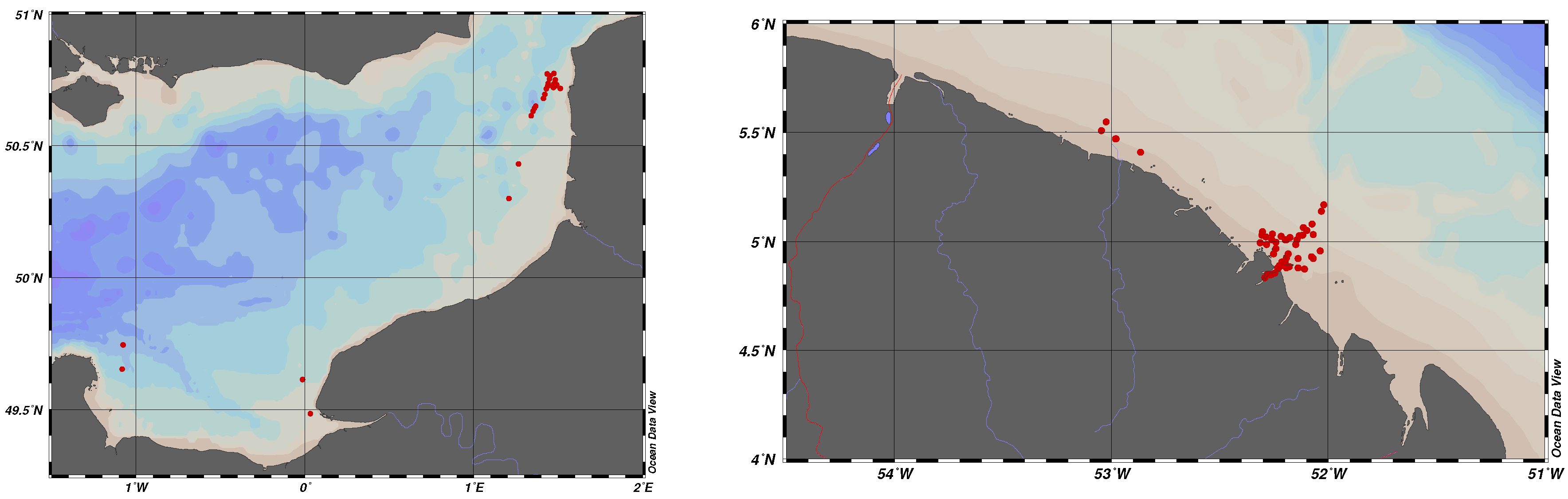
2.2.1. Study Area

The validation of OLCI-A ρ w retrievals is performed using field radiometric measurements collected in two contrasted coastal waters [78]: the Eastern English Channel and French Guiana coastal waters.
Figure 1 shows the location of the stations. For the measurements in the Eastern English Channel (left box of Figure 1), most of the stations are located in the northeast of the English Channel, except two stations in Somme Bay and four other stations in Seine Bay. For measurements in French Guiana (right box of Figure 1), the stations are mostly located in the east part of the coastal waters, near the capital Cayenne, except six located in the Mahury River.
As shown in Table 1, most of the field campaigns were conducted in French Guiana, leading to almost twice more stations and potential match-up numbers than in the Eastern English Channel. However 11 stations were removed in the absence of OLCI-A images. The potential match-ups were made with no additional selecting criteria than the availability of OLCI data.
The Eastern English Channel region has a temperate climate and moderate salinity influenced by the Seine and Escault rivers. This area is influenced by strong tide ranges, river inputs, and low bathymetry, leading to re-suspension of suspended materials, water masses mixing, and relatively intense spring blooms of phytoplankton. These factors make the Eastern English Channel a moderate turbid waters area [79].
The French Guiana region is subject to a tropical climate and to the dominant influence of the Amazon River plus other local rivers such as the Mahury River. This region is influenced by the south-equatorial current. The coastal waters are influenced by a strong fresh water input, very low bathymetry, strong tidal ranges, water masses mixing, and the migration of mud banks [80,81]. For these reasons, the French Guiana coastal waters are considered as very turbid (and sometimes extremely turbid) waters [82].
In these regions, the spatio-temporal distribution of the IOPs is highly variable [83]. In the coastal area of the Eastern English Channel, the bio-optical properties have a pronounced seasonal variation. Relevant differences are observed between winter and spring-summer periods. The CDOM largely dominates the total absorption in winter. In the spring-summer period, the phytoplankton absorption dominates [83]. In French Guiana, the Suspended Particulate Matter (SPM) mainly dominates the IOPs variability, which presents a very high temporal variability with daily high- and seasonal low-frequency variations. High heterogeneity of the optical water types is also observed [84].

2.2.2. Field-Measured Ocean Color Radiometry

The field radiometric measurements were collected using an Analytical Spectral Devices (ASD) FieldSpec 4 Standard-Res spectro-photometer (Analytical Spectral Devices, Inc., Boulder, CO, USA) with a spectral range between 350 and 2500 nm [85,86,87]. The mean nominal spectral resolution was about 3 nm (at 700 nm) and 10 nm (at 1400 nm or 2100 nm). The spectral sampling was about 1.4 nm (350–1000 nm) and 1.1 nm (1001–2500 nm). The scanning time was about 100 milliseconds, and the Field Of View (FOV) was 8 .
The ASD spectro-photometer measures the radiances of the back-scattered light by the water surface L t , the sky L s , and the Spectralon plate L p with a reflecting factor ρ p of about 99% [85,86,87,88], in a similar way as the TriOS-RAMSES above-water system [89,90]. For each measurement, 10 or three (after 3 July 2017) scans by parameter were recorded. Knaeps et al. [85] showed an inter-comparison between ASD and above TriOS system measurements, and overall, the spectra match very well with each other.
The initial sequence of measurements is: L p , L s , L t . For measurements collected from November 2017, the measurement order was changed to: L p , L s , L t , L s , and L p to avoid the high variability of sky and illumination conditions by increasing the measurements of L p and L s .
The viewing geometry of L t and L s measurements were defined with a zenith angle of 45 from the nadir and an azimuth angle of 135 from the Sun plane, keeping the Sun in the back to minimize the sun-glint [85,88]. For L p , the measurement geometry was perpendicular to the Spectralon plate [91]. When possible, the wind speed was measured. To generate the radiances, the radiometric calibration was carried out using the dedicated auxiliary data and software delivered with the ASD spectro-photometer.
After performing the radiometric calibration, the first step of the post-processing protocol consisted of double-checking the quality of the measured radiances L p , L s , and L t . For each station, the coefficient of variation (CV Med ), the standard deviation over the median ratio, were computed at each λ . If CV Med (L x ( λ ) ) was below 5%, 10%, and 10% for x = p , s , and t , respectively, the scans were conserved and used to compute the median value. If not, the relative median absolute difference (RMedD) was computed for each scan (L i , Equation (3)). The scans with values of RMedD(L i ( λ )) equal to or below 10% for L p , L s , and L t were conserved and used to recompute the median Med(L x ( λ )).
RMedD ( L i ( λ ) ) = L i ( λ ) Med ( L x ( λ ) ) Med ( L x ( λ ) ) 100
In a second step, ρ w was calculated using Equation (4) [85,86,88].
ρ w ( λ ) = L t ( λ ) ρ s L s ( λ ) L p ( λ ) ρ p ( λ )
with ρ p ( λ ) the wavelength-dependent Spectralon plate reflectance and ρ s the air-sea interface reflection coefficient, which depends on the wind speed W [89] and is wavelength independent [88]. The spectral variation of ρ p was delivered with the ASD Spectralon plate.
ρ s is computed as a function of W, following the sky plate Spectralon radiances ratio at 750 nm, dL s / p (750 nm), described in Equation (5). If dL s / p (750 nm) is <0.05 for clear sky conditions, ρ p is determined as a function of W, else if dL s / p (750 nm) is ≥0.05 for overcast sky, ρ p received a fixed value. When the wind speed was not available, W was assumed to be moderate and equal to 5 m·s 1 [89]. This led to W ranging between 0.37 and 5 m·s 1 with a mean of 3.97 m·s 1 (±1.70 m·s 1 ).
dL s / p ( 750 nm ) = L s ( 750 nm ) π L p ( 750 nm ) ρ p ( 750 nm )
The final step consists of a visual inspection of the spectrum shape. If the spectrum presents any discontinuity [89] or any anomalous shape, the spectrum is rejected. The quality assurance score (QAS) [92] was used for the selection of the spectra having QAS > 0.66. The QAS procedure is a four-step method. In the first step, the target reflectances are matched with the QAS reference reflectances with regards to the wavelength. In the next step, the target reflectances are normalized. Then, an optical water type is assigned to the target spectra by comparison to the QAS reference ones using the spectral similarity based on the spectral angle [93]. Finally, the total score is computed following the mean of the sum of the spectral scores, which receives a value of one if the target spectral reflectance is in between the upper and the lower boundaries of the QAS reference reflectance [92].

2.2.3. Field-Measured Biogeochemical Parameters

During the sea campaigns, surface water samples were collected. Biogeochemical and bio-optical parameters were measured such as the turbidity and the absorption coefficient of the colored dissolved organic matter ( a C D O M ).
The turbidity was measured using the HACH 2100Qis Portable Turbidimeter (HACH Company, Loveland, CO, USA), which meets the ISO-7027 norm and has a measurement range of 0–1000 Formazin Nephelometric Units (FNU) with a resolution of 0.01 FNU. Before each sea campaign, the turbidimeter was calibrated with the StabCal Formazin Standards. The turbidity was determined by calculating the mean and standard deviation values of ten replica by sample as described in Neukermans et al. [94].
The CDOM spectral absorption coefficient ( a C D O M ( λ ) ) was estimated based on the NASA protocol [95]. The method consists of filtering the seawater sample under a gentle vacuum (<5 in Hg) using a 0.2- μ m polycarbonate membrane. Using a double-beam UV-visible spectrophotometer (Shimadzu UV-2450 (Shimadzu Corporation, Kyoto, Japan)), CDOM absorbance was measured between 250 and 850 nm with 1 nm of spectral resolution. The CDOM absorbance was then used to compute a C D O M . The full details are given in [96].

2.2.4. Remotely-Sensed Ocean Color Radiometry

In the frame of the Sentinel-3 Validation Team, the last released version v2.23 Level-2 (L2) Full Resolution (FR, spatial resolution of 300 m) reprocessed ocean color data and Level-1B (L1B) FR reprocessed top of atmosphere remotely-sensed radiance data were available and used for the validation of the OLCI-A ρ w product. Data from 26 April 2016–November 29, 2017 were downloaded via Copernicus Online Data Access repro (CODArep (https://codarep.eumetsat.int/)). After 30 November 2017, data were collected via the Earth Observation Portal (EO-Portal (https://eoportal.eumetsat.int/)) and Copernicus Online Data Access (CODA (https://coda.eumetsat.int)).
The OLCI-A L2 was used for the validation of BlAC. L1B OCLI was processed using different software: the C2R-CC Processor Version 1.0 plug-in, under the Sentinels Application Platform (SNAP) v6.0 software [76] for C2R-CC and C2R-CCAltNets; the Polymer v4.10 archived package for Polymer [51]; the SeaWIFS Data Analysis System (SeaDAS) v7.5 for NASA [97]. BlAC and Polymer v4.10 were system vicariously calibrated (SVC), while this was not the case for the other ACs. The SVCs of these former AC were performed using Case I water measurements from the MOBY (Marine Optical BuoY) [98] and BOUSSOLE (BOUée pour l’acquiSition d’une Série Optique à Long termE) [99,100].

2.3. Match-Ups Exercise

The goal of a match-up exercise is to co-locate satellite images and in situ measurements in time and space [101]. To perform this comparison, the following steps have been taken into account.

2.3.1. Recommended Flags

The common and usually-used recommended flags for ρ w are: invalid, land, snow-ice, cloud, suspect, high sun-glint, whitecaps, high zenith angle, saturation, and AC failure pixels [101]. Other types of flags were used depending on the AC: the adjacency effect and ρ w negative value between 412 and 665 nm flags for BlAC [36,70,102], out of scope and out of range of atmospheric correction neural nets flags for C2R-CC and C2R-CCAltNets [40,76], negative back-scattering coefficient, out of bounds, exception, thick aerosol, high air mass, and inconsistency flags for Polymer [51,103], and stray light, very low 560-nm water-leaving radiance L w (560 nm) and navigation fail flags for NASA [19,37,77].

2.3.2. Selection Criteria

The match-ups exercise is based on selection criteria [20,21,101,104]. The selection criteria included a time window of ±2 h between the satellite overpass and in situ measurements times. In addition, the image pixels were extracted over a 3-by-3-pixel box centered on the in situ measurements. The number of valid pixels had to be at least 6 out of 9. The mean and the standard deviation of the valid pixels, in the 3-by-3-pixel box, were computed and used to determine the coefficient of variation at 560 nm (CV(560)), which has to be below 20% [101].
If a match-up passed the above-cited selection criteria (±2 h, valid pixels ≥6/9 and CV(560) ≤20%), the median of the pixel box was computed to avoid the outliers.

2.3.3. Statistics Analysis

The assessment of each AC was performed through the calculation of six statistical parameters alongside the scatterplots: the slope ( α ) and the intercept ( β ) of the regression line, the bias (Equation (6)), the relative error (RE, Equation (7)), the root mean squared error (RMSE, Equation (8)), and the correlation coefficient (R 2 ).
Bias = 1 N i = 1 N ( ρ w A C ρ w A S D ) ρ w A S D 100
RE = 1 N i = 1 N ( ρ w A C ρ w A S D ) ρ w A S D 100
RMSE = 1 N i = 1 N ( ρ w A C ρ w A S D ) 2
where N is the number of match-ups, ρ w A C is the water-leaving reflectance retrieved by the atmospheric correction algorithms, and ρ w A S D is the measured water-leaving reflectance using the ASD FieldSpec 4 spectro-photometer.
Full spectral statistical analyses were also performed to assess the full spectral quality of the AC ρ w retrievals: QAS [92], Chi-squared mean [104] ( χ 2 ¯ , Equation (9)), and spectral angle mean [93,105] (SAM, Equation (10)). QAS uses 7 wavelengths: 412, 443, 488, 510, 555, 667, and 687 nm, which are the only QAS reference ρ w wavelengths available and closer to the OLCI spectral bands wavelengths. If a wavelength does not exist for OLCI, the nearest wavelength was taken. This was the case at 448, 555, 665, and 687 nm (490-, 560-, 665-, and 681-nm OLCI spectral bands). χ 2 ¯ uses 11 wavelengths after excluding the 560 nm due to its use for error normalization (see Equation (6)): 400, 412, 490, 510, 620, 665, 674, 681, and 709 nm. SAM uses all 12 visible and NIR wavelengths: 400, 412, 443, 490, 510, 560, 620, 665, 674, 681, 709, and 754 nm.
χ 2 ¯ = 1 N i = 1 N j = 1 11 ( ( X j A C ( i ) X j A S D ( i ) ) 2 X j A S D ( i ) ) ; X j = ρ w ( λ j ) ρ w ( λ 560 n m )
S A M = 1 N i = 1 N a r c c o s ( ρ w A S D ( i ) , ρ w A C ( i ) ρ w A S D ( i ) ρ w A C ( i ) )
where i is the index of the spectrum, j is the index of the λ between 400 and 709 nm excluding the 560-nm wavelength, X j A C and X j A S D are ρ w A C ( λ j ) and ρ w A S D ( λ j ) normalized at 560 nm, respectively, and ρ w A S D , ρ w A C are the dot products of ρ w A S D , ρ w A C , and ρ w A S D . ρ w A C are the Euclidean norms of ρ w A S D and ρ w A C , respectively.
The number of match-ups provides information about the spatial coverage provided by each AC. QAS gives quantification of the full spectrum quality of ρ w retrievals with reference to an internal dataset [92]. QAS values have to be closer to one for the highest quality of retrieved spectra. χ 2 ¯ provides information about the full spectrum relative errors of AC retrievals and has to be null. SAM indicates the mean of the full spectrum difference between the AC retrieved and the field measured ρ w spectra and has to be equal to 0 .

2.3.4. Scoring Scheme

A scoring scheme was adapted from Müller et al. [104] with the aim to rank each AC following its performance in comparison to the other ACs. It was based on the scoring of the α , β , bias, RE, RMSE, R 2 , and N of each algorithm depending on their variation range between the minimum and the maximum values of each statistical parameter score considering all ACs. For example, in Equation (11), the algorithm presenting the closest slope to 1 received the highest score of 1 for a given wavelength λ j . The total score (S t o t ) is the sum of the slope score ( S α , Equation (11)), the intercept score ( S β , Equation (12)), the bias score ( S B i a s , Equation (13)), the RE score ( S R E , Equation (14)), the RMSE score ( S R M S E , Equation (15)), the R 2 score ( S R 2 , Equation (16)), and the N score ( S N , Equation (17)) as a function of wavelength λ j (Equation (18)).
S α ( λ j ) = | 1 α A C ( λ j ) | m a x ( | 1 α ( λ j ) | ) m i n ( | 1 α ( λ j ) | ) m a x ( | 1 α ( λ j ) | )
S β ( λ j ) = | β A C ( λ j ) | m a x ( | β ( λ j ) | ) m i n ( | β ( λ j ) | ) m a x ( | β ( λ j ) | )
S B i a s ( λ j ) = | B i a s A C ( λ j ) | m a x ( | B i a s ( λ j ) | ) m i n ( | B i a s ( λ j ) | ) m a x ( | B i a s ( λ j ) | )
S R E ( λ j ) = R E A C ( λ j ) m a x ( R E ( λ j ) ) m i n ( R E ( λ j ) ) m a x ( R E ( λ j ) )
S R M S E ( λ j ) = R M S E A C ( λ j ) m a x ( R M S E ( λ j ) ) m i n ( R M S E ( λ j ) ) m a x ( R M S E ( λ j ) )
S R 2 ( λ j ) = R 2 A C ( λ j ) m i n ( R 2 ( λ j ) ) m a x ( R 2 ( λ j ) ) m i n ( R 2 ( λ j ) )
S N ( λ j ) = N A C ( λ j ) N ρ w A C ( λ j ) < 0 m a x ( N ( λ j ) N ρ w A C ( λ j ) < 0
S t o t = j = 1 12 ( S α ( λ j ) + S β ( λ j ) + S B i a s ( λ j ) + S R E ( λ j ) + S R M S E ( λ j ) + S R 2 ( λ j ) + S N ( λ j ) )
As 12 wavelengths and seven statistical parameter scores are taken into account, the maximum value of S t o t is 84. Similar to QAS, SAM, and χ 2 ¯ , S t o t quantifies AC performance over the full spectrum of ρ w .

3. Results

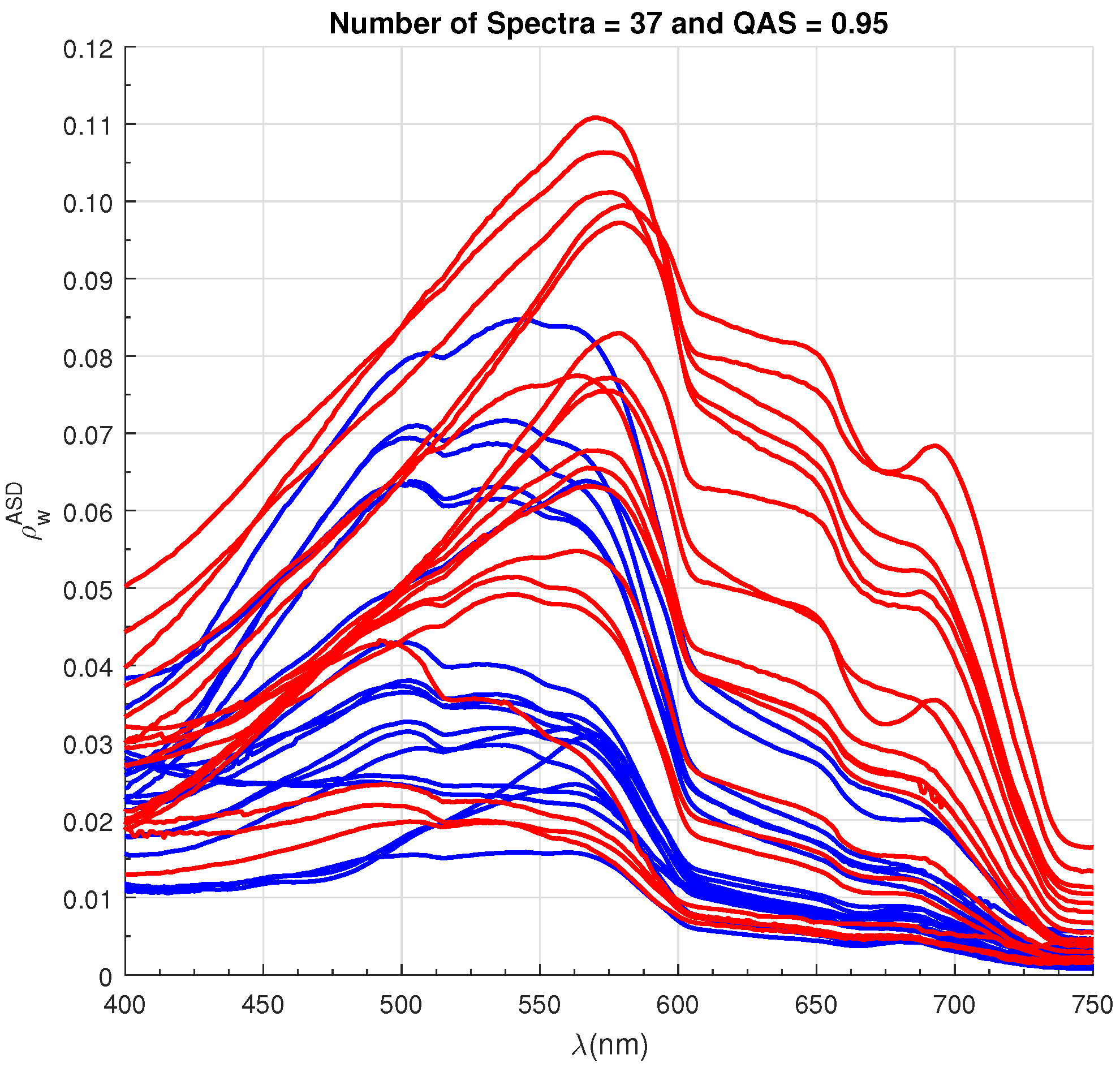
3.1. Field Ocean Color Radiometry

The ASD FieldSpec4 measurement range was between 350 and 2500 nm. We made the choice to show only the 400–750 nm range because it is relevant to commonly-used OLCI spectral bands to access the biogeochemical parameters. Applying all criteria and flags led to obtaining 37 (out of 76) valid match-ups: 18 in the Eastern English Channel and 19 in French Guiana. Figure 2 shows the 37 spectra of ρ w A S D between 400 and 750 nm used for the validation of all ACs. The QAS mean score was calculated to assess the quality of these spectra; its value was 0.95, very close to one, assuring the high quality of our in situ measurements.
The 37 in situ spectra are representative of a large range of bio-optical water types from weakly-turbid to very turbid waters, with a large range of magnitudes at 400 nm and a peak magnitude ranging around 490, 555, or 700 nm (or around 820 nm in French Guiana) [106,107]. The use of the QAS algorithm allowed us to get 10 out of 23 optical water type clusters following the clustering method developed by Wei et al. [92]. The 10 clusters stand for optical water types having their Chl-a between 0.94 and 10.41 mg·m 3 . The obtained clusters were used as a substitute to Chl-a concentration and allowed us to assess the AC accuracy following the optical water type clusters (see Section 4.2).

3.2. AC Overall Analysis

The number of match-ups depends on the selected AC: 18, 16, 19, 35, and 17 for BlAC, C2R-CC, C2R-CCAltNets, Polymer, and NASA, respectively, out of 37 valid match-ups. Figure 3 presents the scatterplots between the in situ ρ w (x-axis) and the estimated ρ w for all AC (y-axis) for λ between 400 and 754 nm. A visual inspection of the scatterplots shows that the accuracy of the retrievals was wavelength-dependent. For λ between 400 and 443 nm, the scattering of the retrievals was quite high for all ACs except C2R-CCAltNets. This is particularly true for λ at 400 nm. For λ between 490 and 674 nm, the scattering tended to decrease, and the AC performances seemed to increase, getting close to each other with increasing wavelength. For λ between 681 and 754 nm, the accuracy decreased, in particular for NASA at 681 nm.
The scatterplots analysis is in accordance with the spectral variation of the statistical parameters (Figure 4). The slope of the regression line, α , increased with the wavelength until 560 nm and flattened for λ greater than 560 nm. It was especially pronounced for NASA where a clear inflection was observed at 443 nm. C2R-CCAltNets presented the closest α values to one at 400 and 510 nm. Between 560 and 681 nm, it was C2R-CC, except at 620 nm (BlAC). For the longest wavelengths (≥709 nm), α was the closest to one for NASA. For most of the ACs, α increased from 400 nm–490 nm, except for C2R-CCAltNets, for which α was always close to one and did not seem to be wavelength-dependent.
The variations of R 2 (bottom right of Figure 4) were similar to those of α , but more pronounced, i.e., steeper increased values from 400–665 nm. All ACs had an R 2 value ≤90% between 400 and 560 nm, C2R-CCAltNets showing the highest values for this spectral range. From 560 nm, NASA presented the highest values, close to 100%.
The magnitude of the bias was wavelength-dependent, while its sign was algorithm-dependent. C2R-CCAltNets showed the lowest values at 400, 560, 620, 665, 674, 681, and 709 nm, whereas Polymer showed the lowest values at 412 nm. For 443 and 510 nm, C2R-CC was the least biased algorithm. BlAC was always negatively biased, while C2R-CCAltNets was always positively biased. For the other ACs, the sign of the bias depended on the wavelength.
RE showed the standard “smiley” shape with high values in the blue and in the red and low values in the green. Both Polymer and C2R-CC showed the lowest RE for all wavelengths, and their spectral variation were less pronounced compared to the other algorithms.
The spectral variation of RMSE was different from the other statistical parameters as its values continuously decreased with wavelength. For λ between 400 and 510 nm, C2R-CC showed the lowest values of RMSE, while the highest values were obtained for BlAC. For λ between 560 and 754 nm, C2R-CC and C2R-CCAltNets showed the lowest values, while the highest values were obtained for Polymer. It is worth noting that ρ w retrievals with NASA were affected by smile effect correction failure at 681 nm with peak of values for α , bias, RE, and RMSE.
BlAC and NASA performed better in French Guiana than in the Eastern English Channel waters. The other ACs performed equally well in both regions.
Table 2 gives the values of QAS, χ 2 ¯ , SAM, and S t o t for each AC for a time window of ±2-h. C2R-CCAltNets had the maximum value of QAS (0.98), while BlAC and NASA had the lowest value (0.82). C2R-CCAltNets and Polymer had the minimum values of χ 2 ¯ (2.28 and 2.00, respectively), while BlAC had the highest (3.30). When the accuracy of the ACs decreased, χ 2 ¯ increased due to the increase of the relative squared errors of the spectral bands normalized at 560 nm. Polymer presented the lowest value of SAM (7.29) and NASA the maximum value (14.60). SAM had to be 0 when the AC spectra were retrieved accurately, leading to a null angle to superpose the AC spectrum on the in situ-measured spectrum. For S t o t , C2R-CCAltNets was the best-performing AC and had the maximum score of 56.46. In second rank, C2R-CC had a value of 51.99. BlAC showed the lowest value of 36.01.

3.3. AC Concomitant Analysis

The preceding section presented the general evaluation of the AC for all match-ups. Here, we present the same analysis, but considering only the common match-ups to all AC. The number of match-ups decreased from 37 to 14; 10 in the Eastern English Channel and four in French Guiana. Figure 5 and Figure 6 are similar to Figure 3 and Figure 4. The trends observed in the previous section were similar when taking only the common match-ups. The retrievals were not accurate for λ between 400 and 443 nm and between 665 and 754 nm, while they were more accurate for λ between 490 and 620 nm.
Furthermore, for the spectral statistics variation, the ACs spectral shapes of the AC common match-ups were similar for α , β , R 2 , and RMSE. Moreover, C2R-CC and especially C2R-CCAltNets statistical performances decreased in comparison to the initial performance analyses, while the accuracy for the other ACs (NASA, BlAC, and Polymer) showed a relative increase. Here, Polymer became the most efficient AC when taking only the AC concomitant match-ups.
Table 3 is similar to Table 2. Taking into account only the common match-ups and the ±2-h time window gives quite a similar analysis in comparison to the other Δ t. C2R-CCAltNets had the highest QAS value (0.99), while BlAC had the lowest value (0.82). For χ 2 ¯ , NASA had the lowest value (2.18), while BlAC had the highest value (4.19).
In terms of SAM, the minimum value was obtained for Polymer (6.80) and the highest for NASA (15.01). For S t o t , Polymer had the maximum value (65.33) followed closely by C2R-CCAltNets (58.05), while BlAC presented the lowest score (36.11). On the common match-ups, the results were slightly different, with Polymer being the most accurate AC on our dataset, closely followed by C2R-CCAltNets. In all cases, the least accurate AC was BlAC.

4. Discussion

4.1. Impacts on the Number of Match-ups

The number of our field-measured OCR was somewhat limited, but the variability of ρ w was high, so we strongly believe that our in situ dataset was representative of a wide range of situations observed over the Eastern English Channel and French Guiana [21,83,84]. This is the reason why we used a ranking scheme and spectral analysis and not only the classic statistical parameters.

4.1.1. Impact of the Time Window

The match-ups exercise was repeated for different time-window values: ±1.5, ±1, and ±0.5 h to assess the ACs behavior in accordance with the time window. Comparing χ 2 ¯ , SAM, and S t o t values for each AC showed that the full spectrum of statistical parameters of each AC was slightly different, except for the shortest time-window for which the ranking based on S t o t changed (Table 1 and Table 2). For Δ t = ±0.5 h, C2R-CC was ranked first, followed by C2R-CCAltNets, and BlAC was still ranked at the last position. Moreover, a shorter time window can lead to better results in terms of S t o t (BlAC, C2R-CC, and NASA for the individual match-ups).
The number of match-ups depends on the selected AC. Furthermore, the time window highly impacts the number of match-ups. The shorter the time window is, the smaller the number of match-ups is: 21, 28, 33, and 45 stations were rejected due to the ±2-, ±1.5-, ±1-, and ±0.5-h time windows, respectively. Furthermore, for the initial time window (±2 h), only 50 stations were valid for match-ups. Based on the value of CV(560), only two stations were rejected for Polymer. For the other ACs, CV(560) was ≤20%.

4.1.2. Impact of the Recommended Flags

The flags used to get the match-ups can impact the number of valid values and the accuracy of the ACs. For instance, Polymer had 13 (out of 48) match-ups that were rejected. The principal flag was the cloud flag (11) and then the inconsistency flag (2), where t* ρ w or ρ a exceeded ρ t o a . Here, the only limitation for Polymer was the cloudy condition. For BlAC, 32 stations were rejected (out of 50) using the recommended flags: cloud (11), cloud margin (10), high solar zenithal angle (4), high glint (13), ρ w negative value between 412 and 665 nm (3), and the 560-nm optical thickness annotation (1). The high glint and clouds were the most limiting flags for BlAC. For NASA, 33 spectra (out of 50) were rejected due to the clouds (24), the high glint (5), the high zenithal angle (5), and the land (5) flags. Concerning C2R-CC and C2R-CCAltNets, both shared the same number of valid and rejected (31) match-ups due to the cloud (22), sun-glint risk (17), and the AC ANN out of scope and range (1) flags. Most of the ACs were highly limited by the high glint, except Polymer. It seems that the cloudy and sun-glinted stations were not flagged in the same way depending on the AC. This led to a different number of valid match-ups. The high solar zenithal angle flag was only limiting for BlAC and NASA. This happened for four stations in the Eastern English Channel. The presence of the high sun-glint situation occurred more often over French Guiana. The cloudy situation was limiting for both areas.

4.2. Sensitivity Studies

Even if any atmospheric and bio-optical parameters were measured during our sea cruises, we tried to understand the limitations of each AC as a function of physical and biogeochemical parameters: optical water type cluster indexes retrieved by QAS (QAS Cluster ID#), turbidity, a C D O M (412), and CV(560) for the valid match-ups of each AC (the figure is not shown here). The goal was to observe if any correlation existed between the statistical parameters and those external parameters.
For instance, the distribution of RE at 412 nm as a function of QAS clusters showed a dependence in the ACs. For BlAC, no trends existed. For NASA (except for one station (in Cluster 8)), RE(412) strongly increased with Chl-a (QAS cluster ID) increase. For Polymer, RE(412) was homogeneously distributed and did not exceed 80%. For both C2R-CC and C2R-CCAltNets, no relationship was observed between RE(412) and the optical water type clusters. In the turbidity-RE(412) scatter analyses, six stations were missing due to the absence of measurements, and one station presented a high relative standard deviation. No trends were observed between RE(412) and the turbidity for C2R-CC and C2R-CCAltNets. A positive relationship was observed for NASA: RE(412) increased with the increase of turbidity. For turbidity greater than 2 NTU, a positive RE(412)-turbidity relationship was observed for Polymer and BlAC. The RE(412)- a C D O M scatter analyses (12 stations were missing) also showed a logarithmic trend for NASA. No trends were observed for the other ACs. Concerning CV(560)-RE(412) scatter analyses, no particular trends were observed for all ACs. Polymer showed the lowest CV(560) in comparison to the other ACs.
This additional sensitivity study revealed no strong trends between physical and biogeochemical parameters and RE (at any wavelengths) such as observed for SeaWIFS by [20]. This suggests that ACs are less sensitive to the biogeochemical parameters. However, it suggests that Polymer can be affected by high values of turbidity where Chl-a and CDOM do not dominate the marine signal. CDOM, Chl-a, and their resulting turbidity (turbidity indirectly resulting from CDOM) could be limiting for NASA due to the use of Chl-a estimates in the Case-2 iteration scheme. The same could not be observed for the BlAC. The lack of atmosphere and more seawater parameter data limited our discussion.
The AC negative values were taken into account in the match-ups exercise and were included in the scatterplots and the statistics calculations except for BlAC between 412 and 665 nm, as applied by the its recommended flags. BlAC had negative values at 400 nm (1), 709 nm (2), and 754 nm (2), while Polymer and NASA had negative values (six and two, respectively) at 709 nm. The presence of negative values did not impact the statistical parameters of the retrievals. No obvious differences are observed between Figure 3 and Figure 7, wherein the negative values were used to compute the statistical parameters. It is worth noting that the SVC was not applied to all ACs except BlAC and Polymer. The absence of the SVC can explain the performance and the increase of the error retrieval for NASA, C2R-CC, and C2R-CCAltNets.

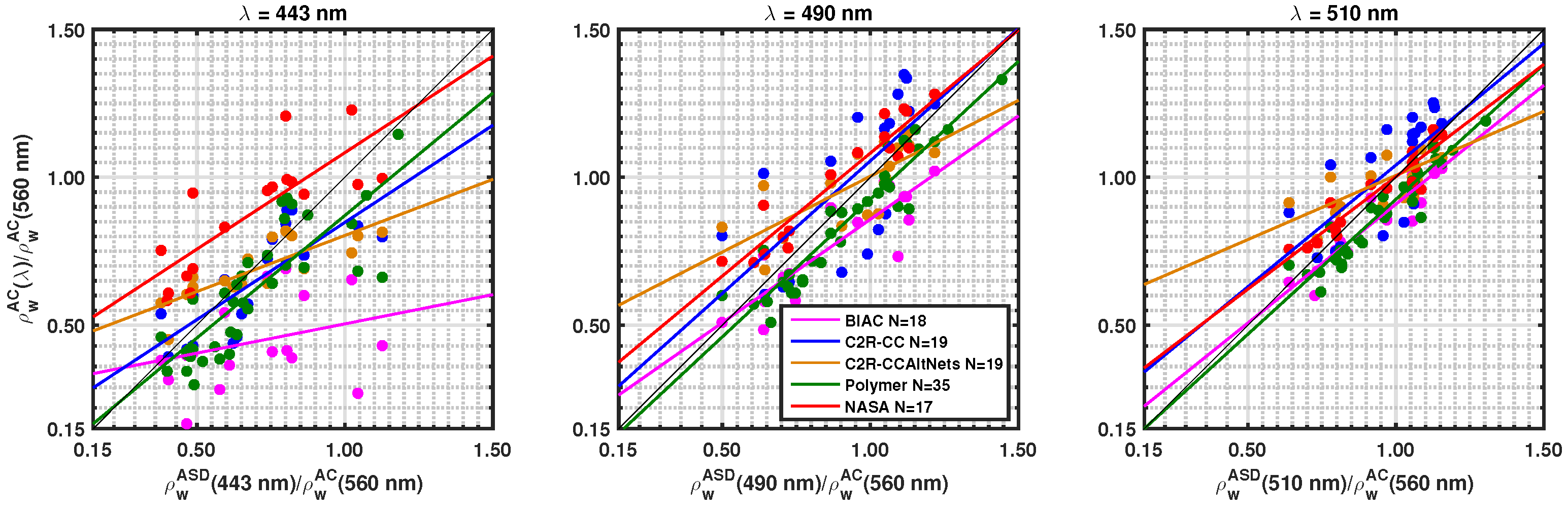
4.3. ACs Band Ratios Performance Impacts

Figure 8 shows the comparison between the water-leaving reflectances ratios for 443/560 nm, 490/560 nm, and 510/560 nm. The spectral bands ratios of AC retrieved and ASD measured ρ w were used to analyze the AC impact on the estimation of the Chl-a, as its estimation is very often based on combination of bands ratios (OC4v4 [108]). Table 4 shows the computed statistical parameters (RE, RMSE, and R 2 ) of the ACs retrieved ρ w 443/560 nm, 490/560 nm, and 510/560 nm bands ratios.
The 443/560-nm ρ w bands ratio match-ups showed the highest differences in terms of RE (34.03, 15.86, 15.85, 16.83, and 37.62% for BlAC, C2R-CC, C2R-CCAltNets, Polymer, and NASA, respectively) and RMSE (0.34, 0.14, 0.14, 0.15, and 0.24 for BlAC, C2R-CC, C2R-CCAltNets, Polymer, and NASA, respectively). The accuracy in the retrieved ratio increased with the increase of the wavelength in the numerator, leading to an accurate estimated ratio for 510/560 nm in terms of statistical values (for instance, R 2 was 84.33, 47.42, 51.77, 89.14, and 88.43% for BlAC, C2R-CC, C2R-CCAltNets, Polymer, and NASA, respectively).
Polymer provided the closest one-to-one regression line for all ratios, as well as the highest R 2 (66.39%, 89.14%, and 89.14% for 443/560 nm, 490/560 nm, and 510/560 nm bands ratios, respectively). BlAC estimates were the least accurate band ratios for 443/560 nm (RE = 34.03% and R 2 = 9.21%) and 490/560 nm (RE = 13.51% and R 2 = 75.74), and it was C2R-CCAltNets for the 510/560-nm ratio (RE = 9.53%, RMSE = 0.11 and R 2 = 51.08%). This is in concordance with the ACs performance inter-comparison results exposed in Section 3.2, and it suggests potentially that the estimation of the Chl-a concentration [108] is impacted by the AC ρ w retrievals (except if the ratio was 510/560 nm).
As the SPM concentration estimation is often based on the use of semi-analytical algorithms (SAA) [109,110,111], it is less impacted by the AC performance if the red spectral band is used in the SPM bio-optical model (560 or 665 nm). Furthermore, all ACs showed the best correlations and lower retrieval errors at the 665-nm spectral band instead of longer wavelengths ( λ > 709 nm). This suggests that the use of the red bands is recommended to estimate the SPM concentration instead of the NIR bands.

4.4. BRDF Effect Issue

The ACs retrieved ρ w were provided without BRDF correction (except for the NASA AC), so the ASD ρ w were not corrected for this effect. Besides, there was still no best solution for this, and it requires, at a given wavelength, a good knowledge of the IOPs, the geometry of observation, the wind speed, and, to a lesser extent, the atmospheric conditions. This correction is proportional to ( Q f ) ( f 0 Q 0 ) ( R 0 R ), where the index 0 stands for the Sun at zenith and a viewing angle at nadir. This factor typically varies between 0.6 and 1.2 [112]. While R 0 R accounts for all transmission and reflection effects at the air-sea interface, the f Q ratios, at a given wavelength, are driven by IOPs and the geometry of observations [113]. Note that the upwelling light fields can only be considered as purely isotropic (which provide a simple solution of the BRDF) for waters with extreme turbidity [114].

5. Conclusions

Validation of OLCI water-leaving reflectance products has been proposed over two contrasted French coastal waters obtained by five different atmospheric correction algorithms. Sea cruises radiometric measurements were collected using a spectro-photometer instrument. Post-processing was developed to assess the quality of the in situ water-leaving reflectances. These in situ measurements were used to conduct a match-up exercise leading to the estimation of statistical parameters and the ranking scheme used in the validation of the water-leaving reflectance retrievals.
The ranking scheme and statistical analysis used in this study show their usefulness for the assessment of the ACs. It allowed us to handle the spectral variations of the statistical parameters from 400–754 nm, which were presented in the match-up exercise results. Furthermore, the ACs performance was taken into account to give in the end a specific AC score that allowed us to rank the ACs following their efficiency. Such a scoring method is highly recommended for the ACs inter-comparison and can be easily extended to the other ocean color retrieval algorithms.
Over our in situ measurements, high performances were obtained for Polymer and C2R-CCAltNets. However, for all ACs, the performance was not very high at 400 and 443 nm. The ACs performances were higher between 490 and 560 nm for all ACs. A sensitivity study was performed to highlight the AC limitations depending on the turbidity or biogeochemical parameters. The sensitivity analysis showed no limitations and correlation with the chosen in-water parameters.
The ease of using the atmospheric correction processors is a very important criterion for the end-users. In terms of the processing time, Polymer had the fastest processing, followed by NASA and both C2R-CC versions. Polymer is recommended for atmospheric correction facility. The standard OLCI AC, BlAC, still needs improvements.
The common match-ups analyses allowed a better direct comparison of the performances of the AC. This allowed avoiding the impact of the ACs specific recommended flags that were used in the AC individual match-ups results. The match-ups number was highly impacted by the flags used, which indirectly impacted the resulting ACs performance assessments and the ACs score ranking. While C2R-CCAltNets was the most accurate AC over the individual match-up exercise, Polymer was the most efficient algorithm for the common match-ups. We recommend using either Polymer or C2R-CCAltNets to process OLCI images over our regions of interest or over similar regions.

Author Contributions

M.A.M. was in charge of collecting and processing the OLCI-A data, collecting and post-processing the ASD field measured data, preparing and analyzing the figures and tables, and pre-writing the manuscript. C.J. was in charge of programming the field cruises alongside V.V. and co-writing and improving the manuscript. H.L., C.J., and V.V. were involved in the development of measurement and post-processing protocols. H.L. and V.V. were involved in the manuscript co-writing. X.M. and A.C. were in charge of turbidity measurements processing. V.V., X.M., and A.C. were in charge of CDOM analysis and data processing. All authors took part in the field biogeophysical parameters and OCR collection during the field cruises.

Funding

The field campaigns were funded by the Centre National d’Etudes Spatiales (CNES) through the TOSCA program, by the Centre National de la Recherche Scientifique (Guyane), and the European Space Agency for the “MERIS validation and algorithm 4th reprocessing” (Contract No. ARG/003-025/1406/LOG). The PhD scholarship fellowship of M.A.M. was funded by the Université du Littoral Côte d’Opale and Région Hauts-de-France. An additional short-term contract of M.A.M. was funded by CNES. The ASD FieldSpec4 was purchased thanks to Université du Littroral-Côte d’Opale through “Bonus Qualité Recherche” and to CNES.

Acknowledgments

The authors would like to thank the Université du Littoral-Côte d’Opale and the Hauts-de-France region for the PhD scholarship fellowship and the CNRS for the short-term contract funding. The European Organization for the Exploitation of Meteorological Satellites (EUMETSAT) is acknowledged for support of the Sentinel-3A data delivery through the Sentinel-3 Validation Team for Ocean Color (S3VT-OC). The authors thank the crew of Wayki village for their help and patience during the field campaigns in French Guiana. The Sepia II and Côte de la Manche ship crews are acknowledged for their help and kindness during sea cruises in the Eastern English Channel. The authors are grateful to David Dessailly for the help in coding the SeaDAS processing loop. Furthermore, the authors would like to thank François Steinmetz for his help in handling the Polymer software and Sean Bailey for his help with the SeaDAS software.

Conflicts of Interest

The authors declare no conflict of interest about the work presented here.

References

  1. Crossland, C.J.; Baird, D.; Ducrotoy, J.P.; Lindeboom, H.; Buddemeier, R.W.; Dennison, W.C.; Maxwell, B.A.; Smith, S.V.; Swaney, D.P. The Coastal Zone—A Domain of Global Interactions. In Coastal Fluxes in the Anthropocene; Crossland, C.J., Kremer, H.H., Lindeboom, H.J., Marshall Crossland, J.I., Le Tissier, M.D.A., Eds.; Springer: Berlin/Heidelberg, Germany, 2005; pp. 1–37. [Google Scholar]
  2. Berger, M.; Moreno, J.; Johannessen, J.A.; Levelt, P.F.; Hanssen, R.F.; Berger, M.; Moreno, J.; Johannessen, J.A.; Levelt, P.F.; Hanssen, R.F. ESA’s sentinel missions in support of Earth system science. Remote Sens. Environ. 2012, 120, 84–90. [Google Scholar] [CrossRef]
  3. Mouw, C.B.; Greb, S.; Aurin, D.; DiGiacomo, P.M.; Lee, Z.; Twardowski, M.; Binding, C.; Hu, C.; Ma, R.; Moore, T.; et al. Aquatic color radiometry remote sensing of coastal and inland waters: Challenges and recommendations for future satellite missions. Remote Sens. Environ. 2015, 160, 15–30. [Google Scholar] [CrossRef]
  4. Morel, A. In-water and remote measurements of ocean color. Bound.-Layer Meteorol. 1980, 18, 177–201. [Google Scholar] [CrossRef]
  5. Morel, A.; Gordon, H.R. Report of the working group on water color. Bound.-Layer Meteorol. 1980, 18, 343–355. [Google Scholar] [CrossRef]
  6. Malenovský, Z.; Rott, H.; Cihlar, J.; Schaepman, M.E.; García-Santos, G.; Fernandes, R.; Berger, M. Sentinels for science: Potential of Sentinel-1, -2, and -3 missions for scientific observations of ocean, cryosphere, and land. Remote Sens. Environ. 2012, 120, 91–101. [Google Scholar] [CrossRef]
  7. IOCCG. Remote Sensing of Inherent Optical Properties: Fundamentals, Tests of Algorithms, and Applications; Reports of the International Ocean Colour Coordinating Group; IOCCG: Dartmouth, NS, Canada, 2006; Volume 5, p. 126. [Google Scholar] [CrossRef]
  8. IOCCG. Why Ocean Colour? The Societal Benefits of Ocean-Colour Technology; Reports of the International Ocean Colour Coordinating Group; IOCCG: Dartmouth, NS, Canada, 2008; Volume 7, p. 141. [Google Scholar]
  9. IOCCG. Remote Sensing in Fisheries and Aquaculture; Reports of the International Ocean Colour Coordinating Group; IOCCG: Dartmouth, NS, Canada, 2009; Volume 8, p. 120. [Google Scholar]
  10. IOCCG. Partition of the Ocean into Ecological Provinces: Role of Ocean-Colour Radiometry; Reports of the International Ocean Colour Coordinating Group; IOCCG: Dartmouth, NS, Canada, 2009; Volume 9, p. 99. [Google Scholar]
  11. IOCCG. Phytoplankton Functional Types from Space; Reports of the International Ocean Colour Coordinating Group; IOCCG: Dartmouth, NS, Canada, 2014; Volume 15, p. 153. [Google Scholar]
  12. IOCCG. Earth Observations in Support of Global Water Quality Monitoring; Reports of the International Ocean Colour Coordinating Group; IOCCG: Dartmouth, NS, Canada, 2018; Volume 17, p. 133. [Google Scholar]
  13. Donlon, C.; Berruti, B.; Buongiorno, A.; Ferreira, M.H.H.; Féménias, P.; Frerick, J.; Goryl, P.; Klein, U.; Laur, H.; Mavrocordatos, C.; et al. The Global Monitoring for Environment and Security (GMES) Sentinel-3 mission. Remote Sens. Environ. 2012, 120, 37–57. [Google Scholar] [CrossRef]
  14. Nieke, J.; Borde, F.; Mavrocordatos, C.; Berruti, B.; Delclaud, Y.; Riti, J.B.; Garnier, T. The Ocean and Land Colour Imager (OLCI) for the Sentinel 3 GMES Mission: Status and first test results. In Proceedings of the Earth Observing Missions and Sensors: Development, Implementation, and Characterization II, Kyoto, Japan, 29 October–1 November 2012; Shimoda, H., Xiong, X., Cao, C., Gu, X., Kim, C., Kiran Kumar, A.S., Eds.; SPIE: Kyoto, Japan, 2012; Volume 8528, p. 85280C. [Google Scholar] [CrossRef]
  15. Frerick, J.; Nieke, J.; Mavrocordatos, C.; Berruti, B.; Donlon, C.; Cosi, M.; Engel, W.; Bianchi, S.; Smith, D. Next generation along track scanning radiometer—SLSTR. In Proceedings of the Remote Sensing System Engineering IV, San Diego, CA, USA, 12–13 August 2012; Ardanuy, P.E., Puschell, J.J., Bloom, H.J., Eds.; SPIE: San Diego, CA, USA, 2012; Volume 8516, p. 851605. [Google Scholar] [CrossRef]
  16. Ruddick, K.; Vanhellemont, Q. Use of the New Olci and Slstr Bands for Atmospheric Correction Over Turbid Coastal and Inland Waters. In Proceedings of the Sentinel-3 for Science Workshop, Venice-Lido, Italy, 2–5 June 2015; Ouwehand, L., Ed.; ESA Special Publication: Venice-Lido, Italy, 2015. Number SP-734 in 734. pp. 1–5. [Google Scholar]
  17. IOCCG. Atmospheric Correction for Remotely-Sensed Ocean-Colour Products; Reports of the International Ocean Colour Coordinating Group; IOCCG: Dartmouth, NS, Canada, 2010; Volume 10, p. 78. [Google Scholar]
  18. Gordon, H.R. Atmospheric correction of ocean color imagery in the Earth Observing System era. J. Geophys. Res. Atmos. 1997, 102, 17081–17106. [Google Scholar] [CrossRef] [Green Version]
  19. Gordon, H.R.; Wang, M. Retrieval of water-leaving radiance and aerosol optical thickness over the oceans with SeaWiFS: A preliminary algorithm. Appl. Opt. 1994, 33, 443. [Google Scholar] [CrossRef] [PubMed]
  20. Jamet, C.; Loisel, H.; Kuchinke, C.P.; Ruddick, K.; Zibordi, G.; Feng, H. Comparison of three SeaWiFS atmospheric correction algorithms for turbid waters using AERONET-OC measurements. Remote Sens. Environ. 2011, 115, 1955–1965. [Google Scholar] [CrossRef]
  21. Goyens, C.; Jamet, C.; Schroeder, T. Evaluation of four atmospheric correction algorithms for MODIS-Aqua images over contrasted coastal waters. Remote Sens. Environ. 2013, 131, 63–75. [Google Scholar] [CrossRef]
  22. Hu, C.; Carder, K.L.; Muller-Karger, F.E. Atmospheric correction of seawifs imagery: Assestement of the use of alternative bands. Appl. Opt. 2000, 39, 3573. [Google Scholar] [CrossRef] [PubMed]
  23. Ruddick, K.G.; Ovidio, F.; Rijkeboer, M. Atmospheric correction of SeaWiFS imagery for turbid coastal and inland waters. Appl. Opt. 2000, 39, 897–912. [Google Scholar] [CrossRef] [PubMed]
  24. Wang, M.; Liu, X. The MODIS-SWIR Algorithm Theoretical Basis Document Version 1.0; NOAA NESDIS STAR, Ed.; Technical Report Feb; College Park, MD, USA, 2012. Available online: https://www.star.nesdis.noaa.gov/sod/mecb/color/documents/SWIR_ATBD_ver1-2012.pdf (accessed on 30 November 2015).
  25. Wang, M. Remote sensing of the ocean contributions from ultraviolet to near-infrared using the shortwave infrared bands: Simulations. Appl. Opt. 2007, 46, 1535. [Google Scholar] [CrossRef] [PubMed]
  26. Shi, W.; Wang, M. An assessment of the black ocean pixel assumption for MODIS SWIR bands. Remote Sens. Environ. 2009, 113, 1587–1597. [Google Scholar] [CrossRef]
  27. Dogliotti, A.; Ruddick, K. Improving water reflectance retrieval from MODIS imagery in the highly turbid waters of La Plata River. In Proceedings of the VI International Conference Current Problems in Optics of Natural Waters (ONW’2011), St. Petersburg, Russia, 6–10 September 2011; pp. 3–10. [Google Scholar]
  28. Chen, J.; Yin, S.; Xiao, R.; Xu, Q.; Lin, C. Deriving remote sensing reflectance from turbid Case II waters using green-shortwave infrared bands based model. Adv. Space Res. 2014, 53, 1229–1238. [Google Scholar] [CrossRef]
  29. He, Q.; Chen, C. A new approach for atmospheric correction of MODIS imagery in turbid coastal waters: A case study for the Pearl River Estuary. Remote Sensing Lett. 2014, 5, 249–257. [Google Scholar] [CrossRef]
  30. Vanhellemont, Q.; Ruddick, K. Advantages of high quality SWIR bands for ocean color processing: Examples from Landsat-8. Remote Sens. Environ. 2015, 161, 89–106. [Google Scholar] [CrossRef]
  31. Oo, M.; Vargas, M.; Gilerson, A.; Gross, B.; Moshary, F.; Ahmed, S. Improving atmospheric correction for highly productive coastal waters using the short wave infrared retrieval algorithm with water-leaving reflectance constraints at 412 nm. Appl. Opt. 2008, 47, 3846–3859. [Google Scholar] [CrossRef]
  32. He, T.; Liang, S.; Wang, D.; Wu, H.; Yu, Y.; Wang, J. Estimation of surface albedo and directional reflectance from Moderate Resolution Imaging Spectroradiometer (MODIS) observations. Remote Sens. Environ. 2012, 119, 286–300. [Google Scholar] [CrossRef]
  33. Moore, G.F.; Aiken, J.; Lavender, S.J. The atmospheric correction of water color and the quantitative retrieval of suspended particulate matter in Case II waters: Application to MERIS. Int. J. Remote Sens. 1999, 20, 1713–1733. [Google Scholar] [CrossRef]
  34. Siegel, D.A.; Wang, M.; Maritorena, S.; Robinson, W. Atmospheric correction of satellite ocean color imagery: The black pixel assumption. Appl. Opt. 2000, 39, 3582. [Google Scholar] [CrossRef]
  35. Stumpf, R.P.; Arnone, R.A.; Gould, R.W.; Martinolich, P.; Ransibrahmanakul, V. Algorithm Updates for the Fourth SeaWiFS Data Reprocessing (2003); Technical Report; Hooker, S.B., Ed.; NASA Goddard Space Flight Center: Greenbelt, MD, USA, 2012. Available online: https://oceancolor.gsfc.nasa.gov/docs/technical/seawifs_reports/postlaunch/PLVol22.pdf (accessed on 5 October 2016).
  36. Lavender, S.J.; Pinkerton, M.H.; Moore, G.F.; Aiken, J.; Blondeau-Patissier, D. Modification to the atmospheric correction of SeaWiFS ocean color images over turbid waters. Cont. Shelf Res. 2005, 25, 539–555. [Google Scholar] [CrossRef]
  37. Bailey, S.W.; Franz, B.A.; Werdell, P.J. Estimation of near-infrared water-leaving reflectance for satellite ocean color data processing. Opt. Express 2010, 18, 7521. [Google Scholar] [CrossRef] [PubMed]
  38. Goyens, C.; Jamet, C.; Ruddick, K.G. Spectral relationships for atmospheric correction II Improving NASA’s standard and MUMM near infra-red modeling schemes. Opt. Express 2013, 21, 21176. [Google Scholar] [CrossRef] [PubMed]
  39. Liang, X.; Ignatov, A. AVHRR, MODIS, and VIIRS radiometric stability and consistency in SST bands. J. Geophys. Res. Oceans 2013, 118, 3161–3171. [Google Scholar] [CrossRef] [Green Version]
  40. Doerffer, R.; Schiller, H. The MERIS case 2 water algorithm. Int. J. Remote Sens. 2007, 28, 517–535. [Google Scholar] [CrossRef]
  41. Schroeder, T.; Behnert, I.; Schaale, M.; Fischer, J.; Doerffer, R. Atmospheric correction algorithm for MERIS above case-2 waters. Int. J. Remote Sens. 2007, 28, 1469–1486. [Google Scholar] [CrossRef]
  42. Fan, Y.; Li, W.; Gatebe, C.K.; Jamet, C.; Zibordi, G.; Schroeder, T.; Stamnes, K. Atmospheric correction over coastal waters using multilayer neural networks. Remote Sens. Environ. 2017, 199, 218–240. [Google Scholar] [CrossRef]
  43. Schiller, H.; Doerffer, R. Neural network for emulation of an inverse model operational derivation of Case II water properties from MERIS data. Int. J. Remote Sens. 1999, 20, 1735–1746. [Google Scholar] [CrossRef]
  44. Chomko, R.M.; Gordon, H.R.; Maritorena, S.; Siegel, D.A. Simultaneous retrieval of oceanic and atmospheric parameters for ocean color imagery by spectral optimization: A validation. Remote Sens. Environ. 2003, 84, 208–220. [Google Scholar] [CrossRef]
  45. Stamnes, K.; Li, W.; Yan, B.; Eide, H.; Barnard, A.; Pegau, W.S.; Stamnes, J.J. Accurate and self-consistent ocean color algorithm: Simultaneous retrieval of aerosol optical properties and chlorophyll concentrations. Appl. Opt. 2003, 42, 939. [Google Scholar] [CrossRef]
  46. Jamet, C.; Thiria, S.; Moulin, C.; Crepon, M. Use of a neurovariational inversion for retrieving oceanic and atmospheric constituents from ocean colar imagery: A feasibility study. J. Atmos. Ocean. Technol. 2005, 22, 460–475. [Google Scholar] [CrossRef]
  47. Brajard, J.; Jamet, C.; Moulin, C.; Thiria, S. Use of a neuro-variational inversion for retrieving oceanic and atmospheric constituents from satellite ocean color sensor: Application to absorbing aerosols. Neural Netw. 2006, 19, 178–185. [Google Scholar] [CrossRef] [PubMed]
  48. Brajard, J.; Moulin, C.; Thiria, S. Atmospheric correction of SeaWiFS ocean color imagery in the presence of absorbing aerosols off the Indian coast using a neuro-variational method. Geophys. Res. Lett. 2008, 35, L20604. [Google Scholar] [CrossRef]
  49. Kuchinke, C.P.; Gordon, H.R.; Harding, L.W.; Voss, K.J. Spectral optimization for constituent retrieval in Case 2 waters II: Validation study in the Chesapeake Bay. Remote Sens. Environ. 2009, 113, 610–621. [Google Scholar] [CrossRef]
  50. Brajard, J.; Santer, R.; Crépon, M.; Thiria, S. Atmospheric correction of MERIS data for case-2 waters using a neuro-variational inversion. Remote Sens. Environ. 2012, 126, 51–61. [Google Scholar] [CrossRef]
  51. Steinmetz, F.; Deschamps, P.Y.; Ramon, D. Atmospheric correction in presence of sun glint: Application to MERIS. Opt. Express 2011, 19, 9783. [Google Scholar] [CrossRef] [PubMed]
  52. Bi, S.; Li, Y.; Wang, Q.; Lyu, H.; Liu, G.; Zheng, Z.; Du, C.; Mu, M.; Xu, J.; Lei, S.; et al. Inland water Atmospheric Correction based on Turbidity Classification using OLCI and SLSTR synergistic observations. Remote Sens. 2018, 10, 1002. [Google Scholar] [CrossRef]
  53. Elterman, L. UV, Visible, and IR Attenuation for Altitudes to 50 Km, 1968; Environmental Research Papers No. 285; Air Force Cambridge Research Laboratories, Ed.; Office of Aerospace Research U.S. Air Force: Bedford, MA, USA, 1968; p. 49. [Google Scholar]
  54. Gordon, H.R.; Brown, J.W.; Evans, R.H. Exact Rayleigh scattering calculations for use with the Nimbus-7 Coastal Zone Color Scanner. Appl. Opt. 1988, 27, 862. [Google Scholar] [CrossRef]
  55. Gordon, H.R.; Wang, M. Surface-roughness considerations for atmospheric correction of ocean color sensors 1: The Rayleigh-scattering component. Appl. Opt. 1992, 31, 4247. [Google Scholar] [CrossRef]
  56. Wang, M. The Rayleigh lookup tables for the SeaWiFS data processing: Accounting for the effects of ocean surface roughness. Int. J. Remote Sens. 2002, 23, 2693–2702. [Google Scholar] [CrossRef]
  57. Wang, M. A refinement for the Rayleigh radiance computation with variation of the atmospheric pressure. Int. J. Remote Sens. 2005, 26, 5651–5663. [Google Scholar] [CrossRef]
  58. Deschamps, P.Y.; Herman, M.; Tanre, D. Modeling of the atmospheric effects and its application to the remote sensing of ocean color. Appl. Opt. 1983, 22, 3751. [Google Scholar] [CrossRef]
  59. Wang, M.; Gordon, H.R. A simple, moderately accurate, atmospheric correction algorithm for SeaWiFS. Remote Sens. Environ. 1994, 50, 231–239. [Google Scholar] [CrossRef]
  60. Wang, M.; Bailey, S.W. Correction of sun glint contamination on the SeaWiFS ocean and atmosphere products. Appl. Opt. 2001, 40, 4790. [Google Scholar] [CrossRef] [PubMed]
  61. Koepke, P. Effective reflectance of oceanic whitecaps. Appl. Opt. 1984, 23, 1816. [Google Scholar] [CrossRef]
  62. Gordon, H.R.; Wang, M. Influence of oceanic whitecaps on atmospheric correction of ocean-color sensors. Appl. Opt. 1994, 33, 7754. [Google Scholar] [CrossRef]
  63. Frouin, R.; Schwindling, M.; Deschamps, P.Y. Spectral reflectance of sea foam in the visible and near-infrared: In situ measurements and remote sensing implications. J. Geophys. Res. Oceans 1996, 101, 14361–14371. [Google Scholar] [CrossRef]
  64. Stramska, M.; Petelski, T. Observations of oceanic whitecaps in the north polar waters of the Atlantic. J. Geophys. Res. 2003, 108, 3086. [Google Scholar] [CrossRef]
  65. Preisendorfer, R.W. Hydrologic Optics; U.S. Department of Commerce, National Oceanic and Atmospheric Administration, Environmental Research Laboratories, Pacific Marine Environmental Laboratory: Honolulu, HI, USA, 1976; Volume I, p. 1757.
  66. Gordon, H.R.; Brown, O.B.; Evans, R.H.; Brown, J.W.; Smith, R.C.; Baker, K.S.; Clark, D.K. A semianalytic radiance model of ocean color. J. Geophys. Res. 1988, 93, 10909. [Google Scholar] [CrossRef]
  67. Yang, H.; Gordon, H.R. Remote sensing of ocean color: Assessment of water-leaving radiance bidirectional effects on atmospheric diffuse transmittance. Appl. Opt. 1997, 36, 7887. [Google Scholar] [CrossRef] [PubMed]
  68. Wang, M. Atmospheric correction of ocean color sensors: Computing atmospheric diffuse transmittance. Appl. Opt. 1999, 38, 451. [Google Scholar] [CrossRef] [PubMed]
  69. Ahmad, Z.; McClain, C.R.; Herman, J.R.; Franz, B.A.; Kwiatkowska, E.J.; Robinson, W.D.; Bucsela, E.J.; Tzortziou, M. Atmospheric correction for NO2 absorption in retrieving water-leaving reflectances from the SeaWiFS and MODIS measurements. Appl. Opt. 2007, 46, 6504. [Google Scholar] [CrossRef] [PubMed]
  70. Antoine, D.; Morel, A. A multiple scattering algorithm for atmospheric correction of remotely sensed ocean color (MERIS instrument): Principle and implementation for atmospheres carrying various aerosols including absorbing ones. Int. J. Remote Sens. 1999, 20, 1875–1916. [Google Scholar] [CrossRef]
  71. Morel, A.; Prieur, L. Analysis of variations in ocean color. Limnol. Oceanogr. 1977, 22, 709–722. [Google Scholar] [CrossRef]
  72. Sathyendranath, S.; Platt, T. Analytic model of ocean color. Appl. Opt. 1997, 36, 2620–2629. [Google Scholar] [CrossRef]
  73. IOCCG. Remote Sensing of Ocean Colour in Coastal, and Other Optically-Complex, Waters; Reports of the International Ocean Colour Coordinating Group; IOCCG: Dartmouth, NS, Canada, 2000; Volume 3, p. 140. [Google Scholar]
  74. Antoine, D.; Morel, A. Relative importance of multiple scattering by air molecules and aerosols in forming the atmospheric path radiance in the visible and near-infrared parts of the spectrum. Appl. Opt. 1998, 37, 2245–2259. [Google Scholar] [CrossRef]
  75. Nobileau, D.; Antoine, D. Detection of blue-absorbing aerosols using near infrared and visible (ocean color) remote sensing observations. Remote Sens. Environ. 2005, 95, 368–387. [Google Scholar] [CrossRef]
  76. Brockmann, C.; Doerffer, R.; Peters, M.; Stelzer, K.; Embacher, S.; Ruescas, A. Evolution of the C2RCC neural network for Sentinel 2 and 3 for the retrieval of ocean color products in normal and extreme optically complex waters. In Proceedings of the Living Planet Symposium 2016, Prague, Czech Republic, 9–13 May 2016; European Space Agency Special Publication: Prague, Czech Republic, 2016; Volume ESA SP, pp. 1–6. [Google Scholar]
  77. Ahmad, Z.; Franz, B.A.; McClain, C.R.; Kwiatkowska, E.J.; Werdell, J.; Shettle, E.P.; Holben, B.N. New aerosol models for the retrieval of aerosol optical thickness and normalized water-leaving radiances from the SeaWiFS and MODIS sensors over coastal regions and open oceans. Appl. Opt. 2010, 49, 5545. [Google Scholar] [CrossRef] [PubMed]
  78. Szeto, M.; Werdell, P.J.; Moore, T.S.; Campbell, J.W. Are the world’s oceans optically different? J. Geophys. Res. Oceans 2011, 116, 1–14. [Google Scholar] [CrossRef]
  79. Lubac, B.; Loisel, H. Variability and classification of remote sensing reflectance spectra in the eastern English Channel and southern North Sea. Remote Sens. Environ. 2007, 110, 45–58. [Google Scholar] [CrossRef]
  80. Vantrepotte, V.; Loisel, H.; Meriaux, X.; Neukermans, G.; Dessailly, D.; Jamet, C.; Gensac, E.; Gardel, A. Seasonal and inter-annual (2002–2010) variability of the suspended particulate matter as retrieved from satellite ocean color sensor over the French Guiana coastal waters. J. Coast. Res. 2011, 1750–1754. [Google Scholar]
  81. Vantrepotte, V.; Gensac, E.; Loisel, H.; Gardel, A.; Dessailly, D.; Mériaux, X. Satellite assessment of the coupling between in water suspended particulate matter and mud banks dynamics over the French Guiana coastal domain. J. S. Am. Earth Sci. 2013, 44, 25–34. [Google Scholar] [CrossRef]
  82. Loisel, H.; Mériaux, X.; Poteau, A.; Artigas, L.F.; Lubac, B.; Gardel, A.; Caillaud, J.; Lesourd, S. Analyze of the inherent optical properties of French Guiana coastal waters for remote sensing applications. J. Coast. Res. 2009, 2, 1532–1536. [Google Scholar] [CrossRef]
  83. Vantrepotte, V.; Brunet, C.; Mériaux, X.; Lécuyer, E.; Vellucci, V.; Santer, R. Bio-optical properties of coastal waters in the Eastern English Channel. Estuar. Coast. Shelf Sci. 2007, 72, 201–212. [Google Scholar] [CrossRef]
  84. Vantrepotte, V.; Loisel, H.; Dessailly, D.; Mériaux, X. Optical classification of contrasted coastal waters. Remote Sens. Environ. 2012, 123, 306–323. [Google Scholar] [CrossRef]
  85. Knaeps, E.; Dogliotti, A.I.; Raymaekers, D.; Ruddick, K.; Sterckx, S. In situ evidence of non-zero reflectance in the OLCI 1020nm band for a turbid estuary. Remote Sens. Environ. 2012, 120, 133–144. [Google Scholar] [CrossRef]
  86. de Moraes Rudorff, N.; Frouin, R.; Kampel, M.; Goyens, C.; Meriaux, X.; Schieber, B.; Mitchell, B.G. Ocean-color radiometry across the Southern Atlantic and Southeastern Pacific: Accuracy and remote sensing implications. Remote Sens. Environ. 2014, 149, 13–32. [Google Scholar] [CrossRef]
  87. Knaeps, E.; Ruddick, K.G.; Doxaran, D.; Dogliotti, A.I.; Nechad, B.; Raymaekers, D.; Sterckx, S. A SWIR based algorithm to retrieve total suspended matter in extremely turbid waters. Remote Sens. Environ. 2015, 168, 66–79. [Google Scholar] [CrossRef]
  88. Mobley, C.D. Estimation of the remote-sensing reflectance from above-surface measurements. Appl. Opt. 1999, 38, 7442. [Google Scholar] [CrossRef] [PubMed]
  89. Ruddick, K.G.; De Cauwer, V.; Park, Y.J.; Moore, G. Seaborne measurements of near infrared water-leaving reflectance: The similarity spectrum for turbid waters. Limnol. Oceanogr. 2006, 51, 1167–1179. [Google Scholar] [CrossRef] [Green Version]
  90. Goyens, C.; Jamet, C.; Ruddick, K.G. Spectral relationships for atmospheric correction I Validation of red and near infra-red marine reflectance relationships. Opt. Express 2013, 21, 21162. [Google Scholar] [CrossRef] [PubMed] [Green Version]
  91. Doxaran, D.; Cherukuru, N.C.; Lavender, S.J.; Moore, G.F. Use of a Spectralon panel to measure the downwelling irradiance signal: Case studies and recommendations. Appl. Opt. 2004, 43, 5981–5986. [Google Scholar] [CrossRef] [PubMed]
  92. Wei, J.; Lee, Z.; Shang, S. A system to measure the data quality of spectral remote sensing reflectance of aquatic environments. J. Geophys. Res. Oceans 2016, 121, 8189–8207. [Google Scholar] [CrossRef]
  93. Kruse, F.; Lefkoff, A.; Boardman, J.; Heidebrecht, K.; Shapiro, A.; Barloon, P.; Goetz, A. The spectral image processing system (SIPS)—Interactive visualization and analysis of imaging spectrometer data. Remote Sens. Environ. 1993, 44, 145–163. [Google Scholar] [CrossRef]
  94. Neukermans, G.; Ruddick, K.; Loisel, H.; Roose, P. Optimization and quality control of suspended particulate matter concentration measurement using turbidity measurements. Limnol. Oceanogr. Methods 2012, 10, 1011–1023. [Google Scholar] [CrossRef] [Green Version]
  95. Mueller, J.L.; Pietras, C.; Hooker, S.B.; Austin, R.W.; Miller, M.; Knobelspiesse, K.D.; Frouin, R.; Holben, B.; Voss, K.J. Ocean Optics Protocols for Satellite Ocean Color Sensor Validation, Revision 4, Volume II: Instrument Specifications, Characterization And Calibration; Ocean Color Web Page; NASA Center for Aerospace Information: Hanover, MD, USA, 2003; Volume II, p. 57.
  96. Vantrepotte, V.; Danhiez, F.P.; Loisel, H.; Ouillon, S.; Mériaux, X.; Cauvin, A.; Dessailly, D. CDOM-DOC relationship in contrasted coastal waters: Implication for DOC retrieval from ocean color remote sensing observation. Opt. Express 2015, 23, 33. [Google Scholar] [CrossRef]
  97. Baith, K.; Lindsay, R.; Fu, G.; McClain, C.R. Data analysis system developed for ocean color satellite sensors. Eos Trans. Am. Geophys. Union 2001, 82, 202. [Google Scholar] [CrossRef]
  98. Clark, D.K.; Yarbrough, M.A.; Feinholz, M.E.; Flora, S.; Broenkow, W.; Kim, Y.S.; Johnson, B.C.; Brown, S.W.; Yuen, M.; Mueller, J.L. MOBY, a radiometric buoy for performance monitoring and vicarious calibration of satellite ocean color sensors: Measurement and data analysis protocols. In Ocean Optics Protocols for Satellite Ocean Color Sensor Validation, Revision 4, Volume VI: Special Topics in Ocean Optics Protocols and Appendices; Mueller, J.L., Fargion, G.S., McClain, C.R., Eds.; NASA Goddard Space Flight Center: Greenbelt, MD, USA, 2003; Volume VI, pp. 3–34. [Google Scholar]
  99. Antoine, D.; Chami, M.; Claustre, H.; d’Ortenzio, F.; Morel, A.; Bécu, G.; Gentili, B.; Louis, F.; Ras, J.; Roussier, E.; et al. BOUSSOLE: A joint CNRS-INSU, ESA, CNES, and NASA Ocean Color Calibration and Validation Activity; NASA Goddard Space Flight Center: Greenbelt, MD, USA, 2003; 59p.
  100. Antoine, D.; Guevel, P.; Desté, J.-F.; Bécu, G.; Louis, F.; Scott, A.J.; Bardey, P. The ‘BOUSSOLE’ Buoy—A New Transparent-to-Swell Taut Mooring Dedicated to Marine Optics: Design, Tests, and Performance at Sea. J. Atmos. Ocean. Technol. 2008, 25, 968–989. [Google Scholar] [CrossRef]
  101. Bailey, S.W.; Werdell, P.J. A multi-sensor approach for the on-orbit validation of ocean color satellite data products. Remote Sens. Environ. 2006, 102, 12–23. [Google Scholar] [CrossRef]
  102. Lavender, S. Sentinel-3 OLCI Marine Handbook; EUMETSAT: Darmstadt, Germany, 2018; p. 38. Available online: http://www.eumetsat.int/website/wcm/idc/idcplg?IdcService=GET_FILE&dDocName=PDF_DMT_907205&RevisionSelectionMethod=LatestReleased&Rendition=Web (accessed on 19 July 2012).
  103. Steinmetz, F.; Ramon, D.; Deschamps, P.Y. ATBD V1—Polymer Atmospheric Correction Algorithm; Technical Report; Plymouth Marine Laboratory: Plymouth, UK, 2016. [Google Scholar]
  104. Müller, D.; Krasemann, H.; Brewin, R.J.; Brockmann, C.; Deschamps, P.Y.; Doerffer, R.; Fomferra, N.; Franz, B.A.; Grant, M.G.; Groom, S.B.; et al. The Ocean Colour Climate Change Initiative: I. A methodology for assessing atmospheric correction processors based on in situ measurements. Remote Sens. Environ. 2015, 162, 242–256. [Google Scholar] [CrossRef]
  105. Keshava, N. Distance metrics and band selection in hyperspectral processing with applications to material identification and spectral libraries. IEEE Trans. Geosci. Remote Sens. 2004, 42, 1552–1565. [Google Scholar] [CrossRef]
  106. Mélin, F.; Vantrepotte, V. How optically diverse is the coastal ocean? Remote Sens. Environ. 2015, 160, 235–251. [Google Scholar] [CrossRef] [Green Version]
  107. Ye, H.; Li, J.; Li, T.; Shen, Q.; Zhu, J.; Wang, X.; Zhang, F.; Zhang, J.; Zhang, B. Spectral classification of the Yellow Sea and implications for coastal ocean color remote sensing. Remote Sens. 2016, 8, 321. [Google Scholar] [CrossRef]
  108. O’Reilly, J.E.; Maritorena, S.; Mitchell, B.G.; Siegel, D.A.; Carder, K.L.; Garver, S.A.; Kahru, M.; McClain, C. Ocean color chlorophyll algorithms for SeaWiFS. J. Geophys. Res. Oceans 1998, 103, 24937–24953. [Google Scholar] [CrossRef] [Green Version]
  109. Nechad, B.; Ruddick, K.G.; Park, Y. Calibration and validation of a generic multisensor algorithm for mapping of total suspended matter in turbid waters. Remote Sens. Environ. 2010, 114, 854–866. [Google Scholar] [CrossRef]
  110. Loisel, H.; Mangin, A.; Vantrepotte, V.; Dessailly, D.; Ngoc Dinh, D.; Garnesson, P.; Ouillon, S.; Lefebvre, J.P.; Mériaux, X.; Minh Phan, T. Variability of suspended particulate matter concentration in coastal waters under the Mekong’s influence from ocean color (MERIS) remote sensing over the last decade. Remote Sens. Environ. 2014, 150, 218–230. [Google Scholar] [CrossRef]
  111. Han, B.; Loisel, H.; Vantrepotte, V.; Mériaux, X.; Bryère, P.; Ouillon, S.; Dessailly, D.; Xing, Q.; Zhu, J. Development of a semi-analytical algorithm for the retrieval of suspended particulate matter from remote sensing over clear to very turbid waters. Remote Sens. 2016, 8, 211. [Google Scholar] [CrossRef]
  112. Mobley, C.D.; Werdell, P.J.; Franz, B.; Ahmad, Z.; Bailey, S.W. Atmospheric Correction for Satellite Ocean Color Radiometry; Technical Report June; NASA Goddard Space Flight Center: Greenbelt, MD, USA, 2016.
  113. Morel, A.; Antoine, D.; Gentili, B. Bidirectional reflectance of oceanic waters: Accounting for Raman emission and varying particle scattering phase function. Appl. Opt. 2002, 41, 6289. [Google Scholar] [CrossRef]
  114. Loisel, H.; Morel, A. Non-isotropy of the upward radiance field in typical coastal (Case 2) waters. Int. J. Remote Sens. 2001, 22, 275–295. [Google Scholar] [CrossRef]
Sample Availability: The ASD field measured OCR data and the corresponding OLCI-A L1B and L2 data are available from the corresponding author under request.
Figure 1. Maps of field OCR measurements locations over the Eastern English Channel (left) and French Guiana (right).
Remotesensing 11 00668 g001
Figure 2. Spectral variation of the in situ ρ w obtained with the ASD spectro-photometer between 400 nm and 750 nm. The blue color represents the Eastern English Channel station, whereas the red one represents the French Guiana stations. The total number of spectra is given in the top of the panel in addition to the mean of the quality assurance score (QAS).
Remotesensing 11 00668 g002
Figure 3. Scatterplots of the match-up exercise of the atmospheric correction algorithm (AC) retrieval and the field measured water-leaving reflectance for 400, 412, 443, 490, 510, 560, 620, 665, 674, 681, 709, and 754 nm. In the multiple scatterplots figure, the field measured OCR ( ρ w A S D ) ) are represented in the x-axis and the water-leaving reflectance AC retrieval ( ρ w A C ) ) is represented in the y-axis. The black solid lines represent the 1:1 line. The colored solid lines show the linear regression lines between the field-measured and AC retrievals of ρ w . The color lines code and the number of match-ups are indicated in the text box of the top left scatterplot ( λ = 400 nm), where magenta, blue, orange, green, and red colors stand for the baseline atmospheric correction algorithm (BlAC), the Case 2 regional coast color atmospheric correction algorithm (C2R-CC), the alternative neural nets of C2R-CC atmospheric correction algorithm (C2R-CCAltNets), Polymer, and NASA, respectively.
Remotesensing 11 00668 g003
Figure 4. Spectral variation of the statistical parameters between 440 and 750 nm: α (top-left), β (top-middle), bias (top-right), RE (bottom-left), RMSE (bottom-middle), and R 2 (bottom-right). The color code is similar to Figure 3 and given in the text box of the top middle subplot in addition to the match-up numbers.
Remotesensing 11 00668 g004
Figure 5. Scatterplots of the AC concomitant match-ups of the AC retrieval and the field measured water-leaving reflectance for 400, 412, 443, 490, 510, 560, 620, 665, 674, 681, 709, and 754 nm. In the multiple scatterplots figure, the field measured OCR ( ρ w A S D ) ) are represented in the x-axis and the water-leaving reflectance AC retrieval ( ρ w A C ) ) are represented in the y-axis. The black solid lines represent the 1:1 line. The colored solid lines show the linear regression lines between the field-measured and AC retrievals of ρ w . The color code is similar to that in Figure 3, and the number of match-ups is indicated in the text box of the left-top scatterplot ( λ = 400 nm).
Remotesensing 11 00668 g005
Figure 6. Statistical properties of the AC concomitant match-ups evolution as a function of wavelength between 400 and 750 nm. The statistical properties: slope ( α ), intercept ( β ), bias, relative error (RE), root mean squared error (RMSE), and correlation coefficient ( R 2 ) are represented in the y-axes in the subplots starting from the left-top subplot until the right-bottom subplot, respectively. The x-axes represents the variation of the wavelength between 400 and 750 nm. The color code is similar to that in Figure 3 and given with the match-ups numbers in the top-middle subplot text box.
Remotesensing 11 00668 g006
Figure 7. Statistical properties without negative values between 400 and 754 of the AC match-ups evolution as a function of wavelength between 400 and 750 nm. The statistical properties: slope ( α ), intercept ( β ), bias, relative error (RE), root mean squared error (RMSE), and correlation coefficient ( R 2 ) are represented in the y-axes in the subplots starting from the left-top subplot until the right-bottom subplot, respectively. The x-axis represents the variation of the wavelength between 400 and 750 nm. The color code is similar to that in Figure 3 and given in the top middle subplot with the match-ups numbers.
Remotesensing 11 00668 g007
Figure 8. Scatterplots of the AC retrieval and the field measured water-leaving reflectance ratios for 443/560 nm, 490/560 nm, and 510/560 nm wavelengths ratios. In situ OCR ratios ( ρ w A S D ( λ ) / ρ w A S D (560 nm)) are represented in the x-axis and the ACs retrieved ratios ( ρ w A C ( λ ) / ρ w A C (560 nm)) in the y-axis. The color code is similar to that in Figure 3, and the number of match-ups is provided in the text box of the middle scatterplot.
Remotesensing 11 00668 g008
Table 1. The number of days, stations, and stations where OLCI data were not available and potential match-ups by study area.
Study AreasDaysStationsNo OLCIPotential Match-Ups
Eastern English Channel11270027
French Guiana14601149
Total25871176
Table 2. Values of QAS, χ 2 ¯ , SAM and S t o t associated with different time windows. N is the number of match-ups and Δ t is the time window. SAM, spectral angle mean.
ACs Δ t (h)NQAS χ 2 ¯ (%)SAM ( ) S tot
BlAC±2180.823.3013.9736.01
±1.5150.833.1114.4234.54
±1110.812.7013.8532.71
±0.5060.792.1212.6236.21
C2R-CC±2190.962.9510.1451.99
±1.5160.982.8010.6554.22
±1130.982.3409.7756.51
±0.5080.981.4608.0159.81
C2R-CCAltNets±2190.982.2808.5156.46
±1.5160.982.2309.1755.08
±1130.981.8108.5855.45
±0.5080.981.0707.4851.95
Polymer±2350.902.0007.2944.58
±1.5290.922.1407.1642.92
±1250.912.1006.8841.37
±0.5130.891.4507.1137.05
NASA±2170.822.6714.6040.34
±1.5130.842.4014.2440.96
±1100.872.5513.9339.83
±0.5060.862.4114.0142.94
Table 3. Values of QAS, χ 2 ¯ , SAM, and S t o t associated with different time windows and the AC common match-ups. N is the number of match-ups, and Δ t is the time window.
ACs Δ t (h)NQAS χ 2 ¯ (%)SAM ( ) S tot
BlAC±2140.824.1913.8836.11
±1.5120.853.8513.7132.02
±1090.813.2713.4031.08
±0.5050.802.5012.4335.22
C2R-CC±2140.973.8411.4451.63
±1.5120.983.7111.9452.62
±1090.973.3611.0855.24
±0.5050.972.2909.0855.19
C2R-CCAltNets±2140.992.9309.2458.05
±1.5120.992.8309.8557.52
±1090.982.4209.2354.54
±0.5050.971.4307.5553.47
Polymer±2140.932.5606.8065.33
±1.5120.922.4406.7963.07
±1090.922.2206.1165.26
±0.5050.911.4705.3366.40
NASA±2140.832.1815.0147.67
±1.5120.852.0414.4648.38
±1090.892.0814.1947.07
±0.550.891.5414.4845.26
Table 4. Values of RE, RMSE, and R 2 associated with BlAC, C2R-CC, C2R-CCAltNets, Polymer, and NASA retrievals for 443/560 nm, 490/560 nm, and 510/560 nm ratios.
ρ w ASD (443 nm)/ ρ w ASD (560 nm) ρ w ASD (490 nm)/ ρ w ASD (560 nm) ρ w ASD (510 nm)/ ρ w ASD (560 nm)
ACsRE (%)RMSER 2 (%)RE (%)RMSER 2 (%)RE (%)RMSER 2 (%)
BlAC34.030.349.2113.510.1575.749.050.1084.33
C2R-CC15.860.1464.0620.210.1948.4512.970.1447.42
C2R-CCAltNets15.850.1464.4413.260.1357.089.530.1151,77
Polymer16.830.1566.399.900.1089.148.320.0989.14
NASA37.620.2464.1013.850.1289.725.610.0688.43

