Article

Sentinel-3A SRAL Global Statistical Assessment and Cross-Calibration with Jason-3

1
First Institute of Oceanography, Ministry of Natural Resources, Qingdao 266061, China
2
School of Data Science and Software Engineering, Qingdao University, Qingdao 266071, China
*
Author to whom correspondence should be addressed.
Remote Sens. 2019, 11(13), 1573; https://doi.org/10.3390/rs11131573
Submission received: 20 May 2019 / Revised: 30 June 2019 / Accepted: 1 July 2019 / Published: 3 July 2019

Abstract

:
The Sentinel-3A satellite, equipped with Synthetic Aperture Radar (SAR) Altimeter (SRAL) instrument to derive sea surface height, significant wave height and surface wind speed over the global ocean, was launched on 16 February 2016. The assessment of data quality and the system performance of the altimeter are very important to data application. In this article, Sentinel-3A SRAL data quality is assessed and altimetry system performance is estimated by verifying data availability and monitoring the parameters of altimeter and radiometer through the global statistical analyses of Sentinel-3A Non-Time-Critical (NTC) Marine Level 2 products during the period from 13 March 2016 to 25 February 2019, in comparison with self-crossovers and cross-calibration with the Jason-3 mission. The global statistical analyses and the comparisons at self-crossovers show that Sentinel-3A SRAL data and performance are stable and have no trend over time, and the total cycle average root mean square errors (RMSEs) of sea surface height (SSH) differences at self-crossovers is about 5.4 cm. The comparisons at the dual-crossovers show the consistency of the observation between Sentinel-3A SRAL and Jason-3, and indicate that the systemic bias of SSH is about 2.96 cm. In general, it can be concluded that Sentinel-3A SRAL has good and stable data quality and system performance for operational ocean forecasting and scientific research.

Graphical Abstract

1. Introduction

Sentinel-3 is an Earth observation satellite mission of the Copernicus programme which, previously known as GMES (Global Monitoring for Environment and Security), is the European Programme for the establishment of a European capacity for Earth Observation. The Sentinel-3 mission is jointly operated by the European Space Agency (ESA) and the European Organization for the Exploitation of Meteorological Satellites (EUMETSAT) to ensure the long-term collection and operational delivery of high-quality measurements to ocean, land and atmospheric services. The main objective of the Sentinel-3 mission is to measure sea surface topography, sea and land surface temperature, and ocean and land surface color with high accuracy and reliability in order to support ocean forecasting systems, environmental monitoring and climate monitoring [1,2]. The Sentinel-3A satellite was launched on 16 February 2016. Sentinel-3A is a sun-synchronous polar-orbiting satellite operating at a mean altitude of 815 km and an inclination of 98.6°. The Sentinel-3B satellite was launched on 25 April 2018. In addition to the Sentinel-3 mission, the Copernicus programme also includes the Sentinel-1 and Sentinel-2 missions. The Sentinel-1 mission carries a C-band synthetic-aperture radar instrument which provides a collection of data in all-weather, day or night. The Sentinel-2 mission systematically acquires optical imagery at high spatial resolution over land and coastal waters.
The SAR Altimeter (SRAL) instrument is equipped on Sentinel-3A to derive sea surface height (SSH), significant wave height (SWH) and surface wind speed over the global ocean at an accuracy and precision equivalent to that formerly achieved by ENVISAT Radar Altimeter-2 (RA-2), but with enhanced surface topography measurements in the coastal zones, sea ice regions and over inland rivers and lakes. The SRAL instrument is a dual-frequency (Ku- and C-band) nadir-looking radar altimeter that employs SAR altimetry technologies inherited from the CryoSat-2 mission. The technical characteristics of the Sentinel-3A SRAL instrument are shown in Table 1. The Sentinel-3A mission is also equipped with a microwave radiometer used for wet tropospheric correction and an on-board precise orbit determination (POD) system composed of a GPS receiver and a Laser Retro-Reflector for accurate orbit determination. Sentinel-3A has a repeat cycle of 27 days in order to provide a global ocean topography, as well as significant wave height and wind speed measurements. The measurement modes of the SRAL are composed of two radar modes associated with two tracking modes. The two radar modes are Low Resolution Mode (LRM) and SAR mode. LRM is a conventional altimeter pulse limited mode based on a 3Ku/1C/3Ku pulse pattern and SAR mode is a high along-track resolution mode composed of bursts of 64 Ku-band pulses surrounded by 2 C-Band pulses [3]. However, as only one operational mode can be used at a given time, and as the ability to emulate LRM from the SAR mode is developed by the reduced SAR mode technique, which results in pseudo-LRM (PLRM), SRAL works always in SAR mode.
Altimeter data with high accuracy are required by scientific research and operational oceanography. Calibration and validation activities are an important part of any satellite altimetry mission. The main activities of the calibration and validation are intrinsic mono-mission monitoring, cross-calibration with other altimeter missions, and comparison with external data such as tide gauge data or buoy data. Cross-calibration with other missions enables the detection of instrument drifts and inter-mission biases, which are essential to obtaining a consistent multi-satellite data set. A precise calibration between missions, as well as the careful monitoring of the mission performance over time is crucial to ensuring the continuity of the historical satellite altimeter record and allowing the combination of different altimeter mission data to obtain the essential data for operational oceanography [4]. The calibration and validation of Jason-1 [5,6,7], Jason-2 [8,9], Envisat [10] and SARAL/Altika [11,12] are conducted to assess the data quality and to estimate the altimeter system performance. The data quality of the Sentinel-3 mission is validated by the validation and calibration team, and the data product quality reports are disseminated. Each report covers a period of 27 days and the details of each Sentinel-3 orbital cycle are available. The reports summarize the assessment of the altimetry mission, split per instrument, or thematic topic: SRAL, MWR, Ocean Validation, Winds & Waves, and Land & Sea Ice. The Ocean Validation reports summarize validation results obtained from SRAL/Sentinel-3 STC Marine Level 2 products processed by the Marine Centre by monitoring the following parameters: Sea Level Anomaly (SLA), Significant Wave Height, Backscattering Coefficient, and Altimeter Wind Speed [13].
This paper focuses on the long-term monitoring of the Sentinel-3A SRAL system over the ocean. It includes continuous monitoring of altimeter and radiometer parameters, performance assessment, geophysical evaluation, and cross-calibration with Jason-3 measurements, which are not conducted in the routine validation work of Sentinel-3A SRAL. Jason-3 has been validated to have good data quality, like its predecessor Jason-2 [14]. There are four sections in this paper. Section 1 is the introduction. Section 2 is the description of the data and methods used in this study. Section 3 is the data quality analysis of Sentinel-3A SRAL, including the validation of the data, the analysis of the key altimeter and radiometer parameters and the assessment of mission performance using Sea Level Anomaly (SLA) differences at crossovers. The conclusions are summarized in Section 4.

2. Data and Methods

2.1. Sentinel-3A Data

The Sentinel-3A SRAL Non-Time-Critical (NTC) Marine Level 2 products from 13 March 2016 to 25 February 2019 (Cycle 3-41) are used in this study. These data are distributed by EUMETSAT through Copernicus Online Data Access (https://coda.eumetat.int/#/home (after 20 January 2018) and https://codarep.eumetat.int/#/home (before 20 January 2018)). Every complete product contains three NetCDF files, which are reduced measurement, standard measurement and enhanced measurement data [15]. Reduced measurement data contain a subset of the main 1 Hz data. Standard measurement data contain standard 1 Hz and 20 Hz Ku and C band parameters. Enhanced measurement data contain additional information, the waveforms, and the necessary parameters to reprocess the data, in addition to the standard measurement information. The standard measurement data of SRAL products are used in this study. Only the Ku-band SAR and PLRM mode data are selected in the study. Thresholds used for the main altimeter and radiometer parameters in the Sentinel-3A SRAL data editing procedures are shown in Table 2.

2.2. Jason-3 Data

Jason-3 Geophysical Data Records (GDRs) data from 27 February 2016 to 13 January 2019 (Cycle 2-107) distributed by CNES (Centre national d’études spatiales) AVISO (Archiving, Validation and Interpretation of Satellite Oceanographic Data) (ftp://avisoftp.cnes.fr) are used in this study. Jason-3 is an international cooperative satellite altimeter mission between the National Aeronautics and Space Administration (NASA), National Oceanic and Atmospheric Administration (NOAA), EUMETSAT and CNES. Jason-3, which was launched on 17 January 2016, is the successor to the Jason-2, Jason-1 and T/P mission, which measured ocean surface topography, SWH and wind speed from 1992 to the present. These satellites’ mission is to provide a unique global view of the oceans and to supply data for scientific and practical applications to sea level rise, ocean circulation and climate change. The Jason-3 satellite altimeter operates at the Ku and C bands. Jason-3 has a repeat cycle of approximately 10 days. Ku-band data of Jason-3 is used in the assessment of Sentinel-3A SRAL data based on comparisons between Sentinel-3A and Jason-3.

2.3. Data Analysis Methods

Sentinel-3A SRAL data are evaluated by the cycle based on cycle global statistical analyses of Sentinel-3A SRAL data, comparisons at the self-crossovers of Sentinel-3A SRAL, and comparisons between Sentinel-3A and Jason-3. The statistical analyses include the cycle by cycle calculation and comparison of the means and standard deviations of parameters. The means and standard deviations of the parameters of Sentinel-3A SRAL data are computed using the following expression.
a m e a n = 1 N i = 1 N a i
a S D = 1 N i = 1 N ( a i a m e a n ) 2
where ai is the ith value of parameter a during the given time period. N is the total observation number. amean and aSD are the mean and standard deviation of a.
The first step of the comparisons at the self-crossovers and dual-crossovers is to determine the crossover. Ground-track crossover points are selected when the time difference between the measurements of the two altimeter passes is less than a given duration. The crossover points and their parameter data are obtained by bilinear interpolation of four points at the two altimeter passes closest to the crossover point. For the comparison at the self-crossovers, the measurement time differences at the self-crossovers are refined to less than 9 h to obtain more collocated data, which is significantly less than the routine validation work of 10 days [9]. For the comparisons at the dual-crossovers between Sentinel-3A SRAL and Jason-3, the measurement time differences between the two altimeters are confined to less than 30 min based on the result analysis of the differences between the different measurement times (not shown here). Figure 1 shows the schematic diagram of the spatial distribution of self-crossovers with a time difference of less than 9 h and dual-crossovers with a time difference of less than 30 min.
The differences in parameters between SAR and PLRM modes of Sentinel-3A SRAL at the self-crossovers or dual-crossovers are compared cycle by cycle and their biases and root-mean-square errors (RMSEs) are calculated using the following expression.
b i a s = 1 N i = 1 N ( a i b i )
R M S E = 1 N i = 1 N ( a i b i ) 2
where ai and bi are the ith collocated data of SAR or PLRM mode parameter in the given time period. N is the total number of collocated data pairs. The bias and RMSE are the bias and root mean square error of the differences of parameter a and b.

3. Results and Discussion

To evaluate the global performance of Sentinel-3A SRAL, the edited measurements of Sentinel-3A SRAL, the parameters of SRAL, and the radiometer, including wet tropospheric correction, dual frequency ionospheric correction, Sea State Bias (SSB) correction, Significant Wave Height (SWH), backscattering coefficient (Sigma0), wind speed and Sea Level Anomaly (SLA), are analyzed statistically. The following comprise the detailed statistical analyses and comparisons of the parameters of Sentinel-3A mentioned above.

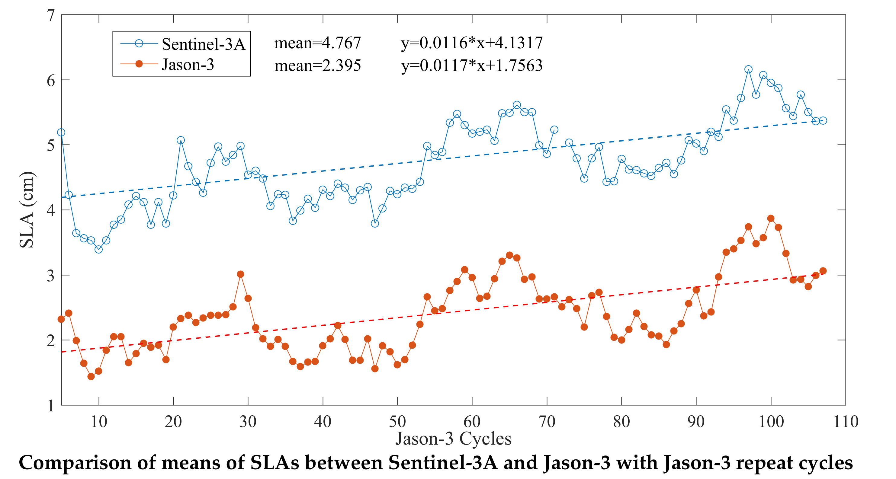
3.1. Edited Measurements

Data editing is necessary to obtain valid measurements. The analysis of the edited measurement of Sentinel-3A SRAL can validate the availability of Sentinel-3A SRAL data. The corresponding cycle by cycle percentages of rejected measurement based on some of the editing criteria of different parameters (as shown in Table 2) in the ocean are presented in Figure 2. These parameters include the number of 20 Hz range measurements, the standard deviation of 20 Hz range measurements, radiometer wet tropospheric correction, dual frequency ionospheric correction, SWH, Sigma0, the number of Sigma0 measurements, and the standard deviation of Sigma0 measurements. The rejected measurements are related the measurement of the backscattering coefficient, SWH and some parameters related to SSH calculation. As shown in Figure 2, most of percentages of the rejected measurements are less than 1%, except for the standard deviation of 20 Hz Sigma0 measurements, and their variabilities, with a total mean of less than 0.63% over time, are stable. The percentage of the standard deviation of 20 Hz Sigma0 measurements is less than 3%, and it has a slight descending trend, with a total mean of less than 1.7%. The analysis of edited measurements shows that the measurements of Sentinel-3A SRAL are stable with high data availability in the ocean.
To analyze the performance of Sentinel-3A SRAL measurements, the cycle by cycle means of the number and standard deviation of 20 Hz range measurements of Sentinel-3A SRAL are compared to those of Jason-3 based on Jason-3 cycles, as shown in Figure 3. It is shown in Figure 3 that the number of 20 Hz range measurements of Sentinel-3A SRAL is larger than that of Jason-3, and the standard deviation of 20 Hz range measurements of Sentinel-3A SRAL is less than that of Jason-3. The total cycle average of the number of 20 Hz range measurements of 19.85 for Sentinel-3A is larger than that of Jason-3 of 19.63. The total cycle average of standard deviation of 20 Hz range measurements of 5.69 cm is less than that of Jason-3 of 7.98 cm. The comparisons of standard deviation of number and standard deviation of 20 Hz range measurements between Sentinel-3A SRAL and Jason-3 (not shown here) present the same results. These results show that Sentinel-3A SRAL has better measurement performance and data availability than Jason-3.

3.2. Cycle by Cycle Statistical Analyses

Based on Sentinel-3A cycle, cycle by cycle global statistical analyses of Sentinel-3A SRAL parameters including wet tropospheric correction, ionospheric correction, sea state bias (SSB) correction, SWH, backscattering coefficient (Sigma0), wind speed and sea surface height (SSH) are conducted to evaluate the stability and accuracy of Sentinel-3A SRAL data.

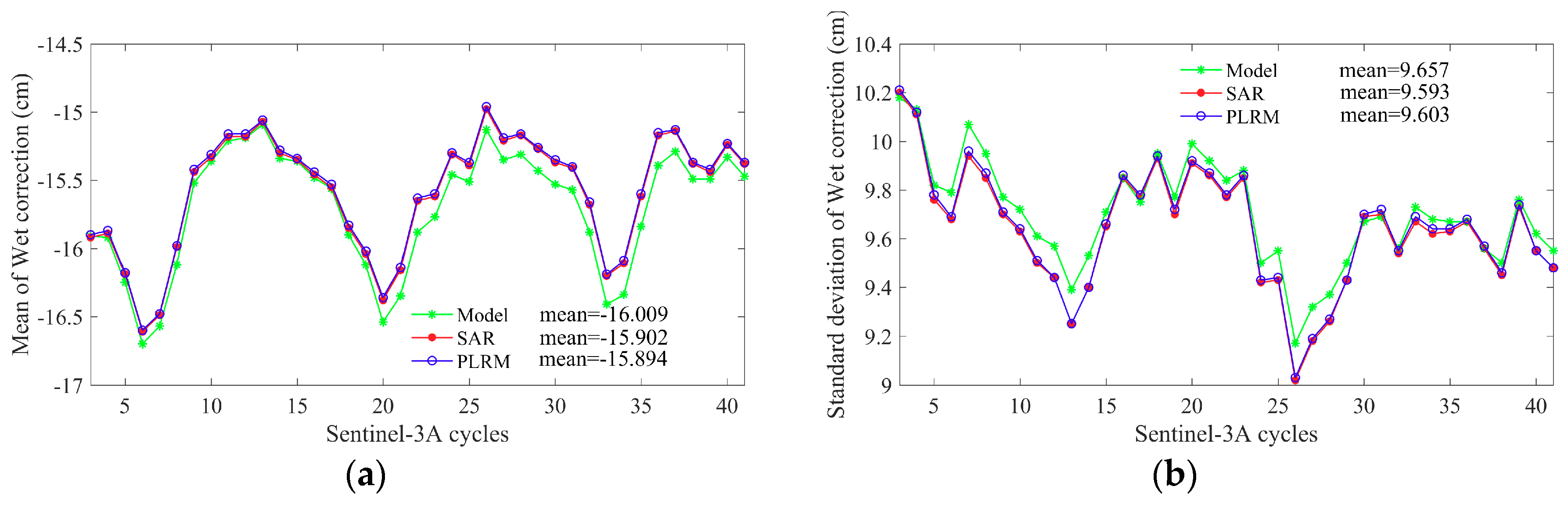
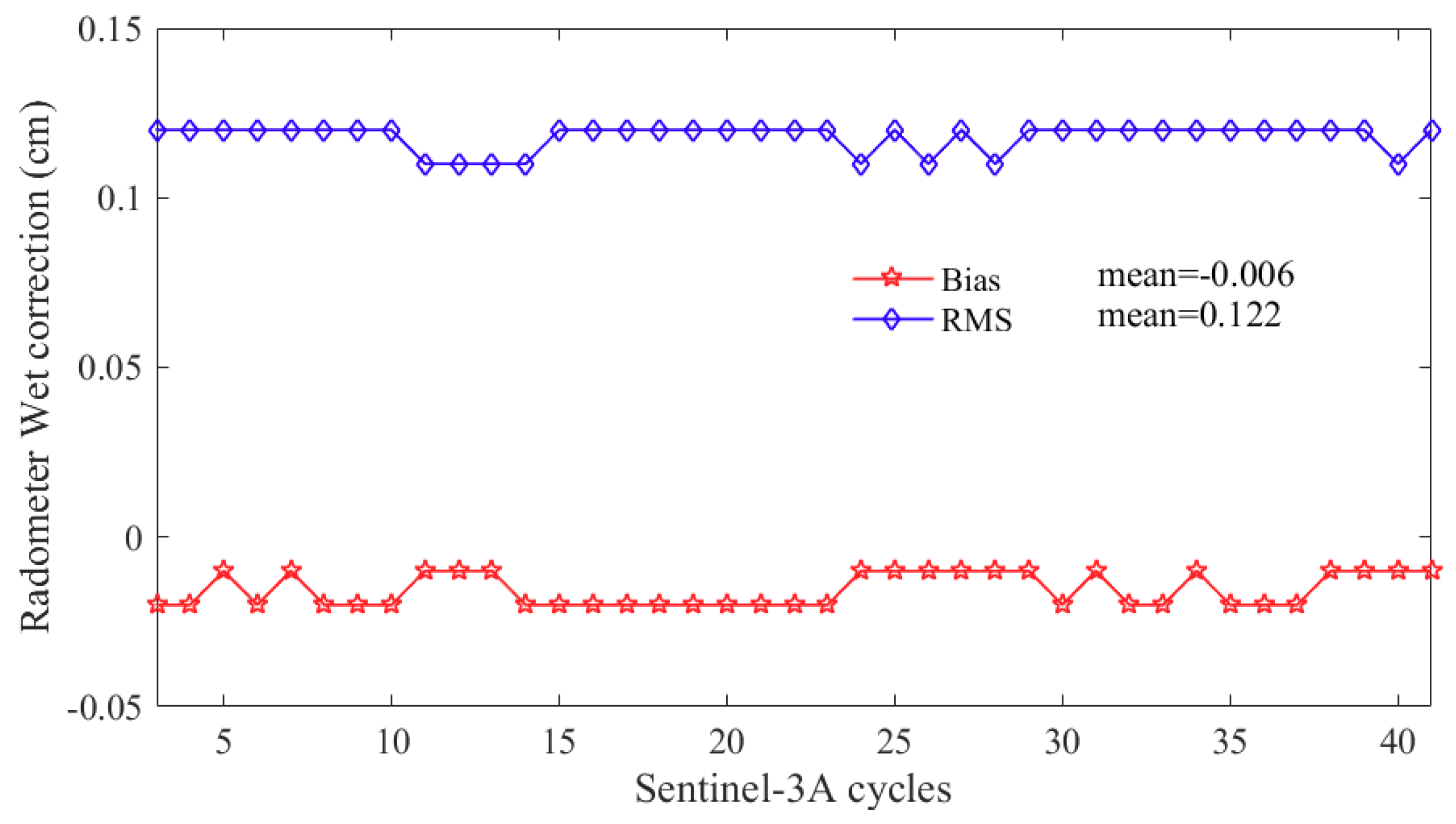
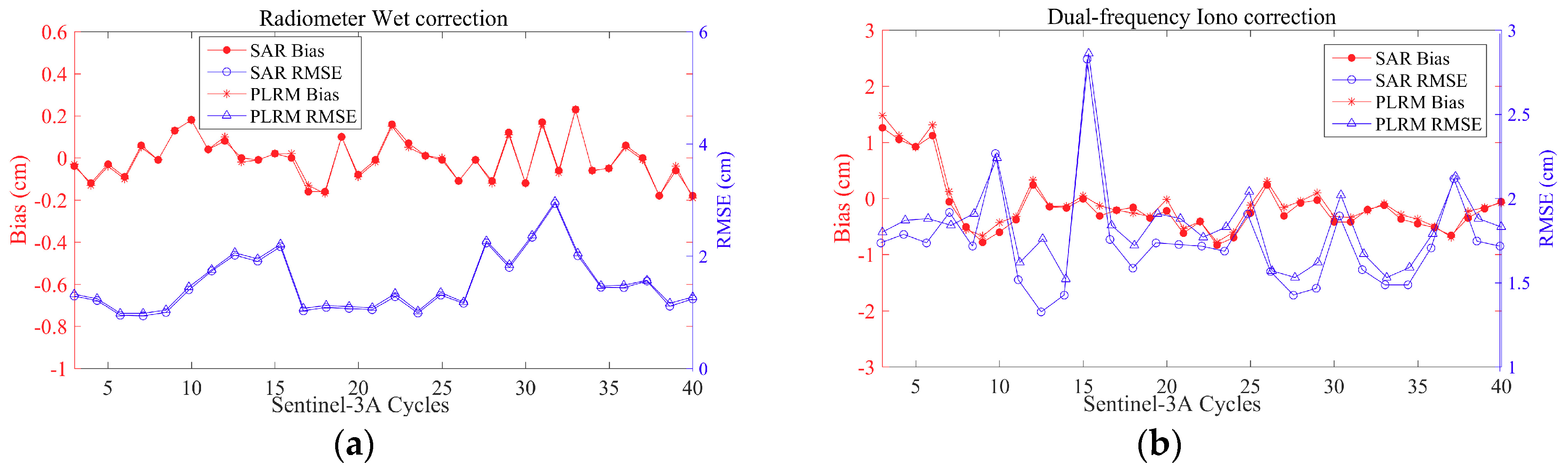
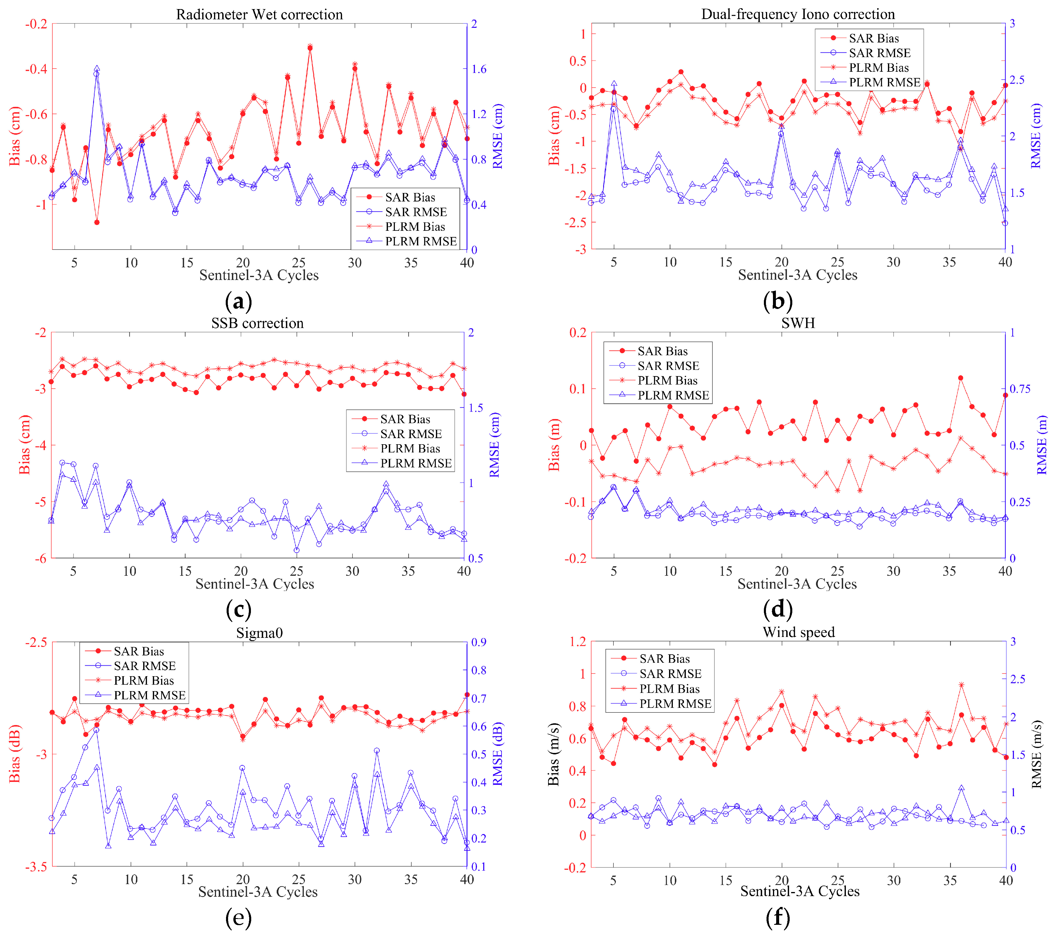
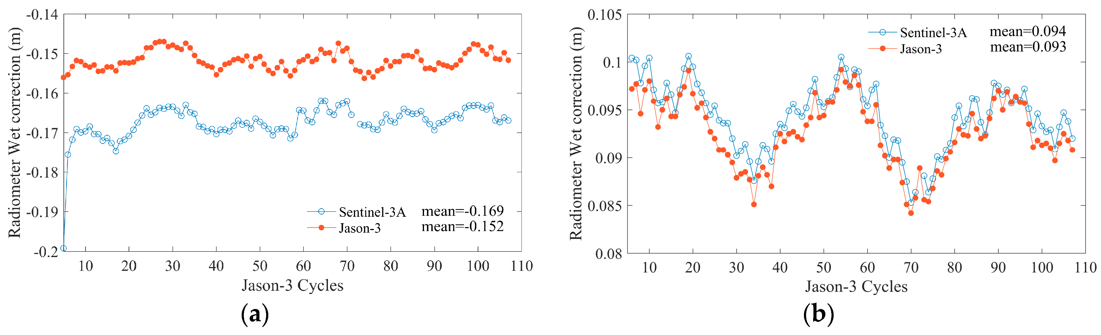
3.2.1. Wet Tropospheric Correction

The wet tropospheric path delay is the delay effect of the altimeter pulse signal due to the water vapor and cloud liquid water in the atmosphere. It is usually corrected by the atmospheric model or the measurement of the radiometer. Three kinds of wet tropospheric corrections, including model, SAR mode and PLRM mode, are compared and analyzed. The cycle by cycle means and standard deviations of the wet tropospheric corrections based on the Sentinel-3A repeat cycles are compared in Figure 4. It is shown that the change of means of wet tropospheric corrections has a period of about one year, and local minima in cycle 7, cycle 20 and cycle 33. This is relative to the annual cyclic variations of water vapor and cloud liquid water in the atmosphere. Global atmospheric water vapor content reaches a maximum in summer, and wet tropospheric correction also reaches a maximum value [16]. There is a small difference between model and radiometer wet tropospheric correction. Cycle by cycle standard deviations of wet tropospheric correction show the stabilities of wet tropospheric corrections, and there is no obvious trend or drift with time. The cycle by cycle biases and RMSEs of differences between SAR and PLRM mode radiometer wet tropospheric correction are shown in Figure 5. SAR mode radiometer wet tropospheric correction has a systemic bias of -0.006 cm relative to that of PLRM mode. The variations of bias and RMSE have no trend. This indicates the stability of Sentinel-3A’s performance.

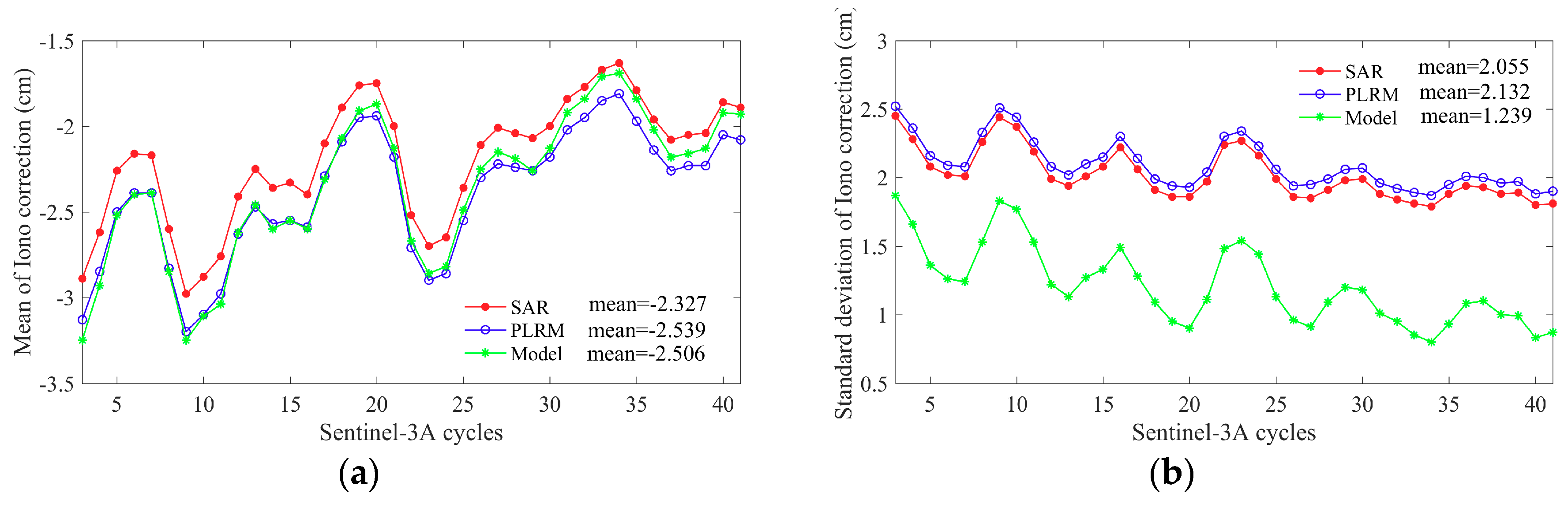
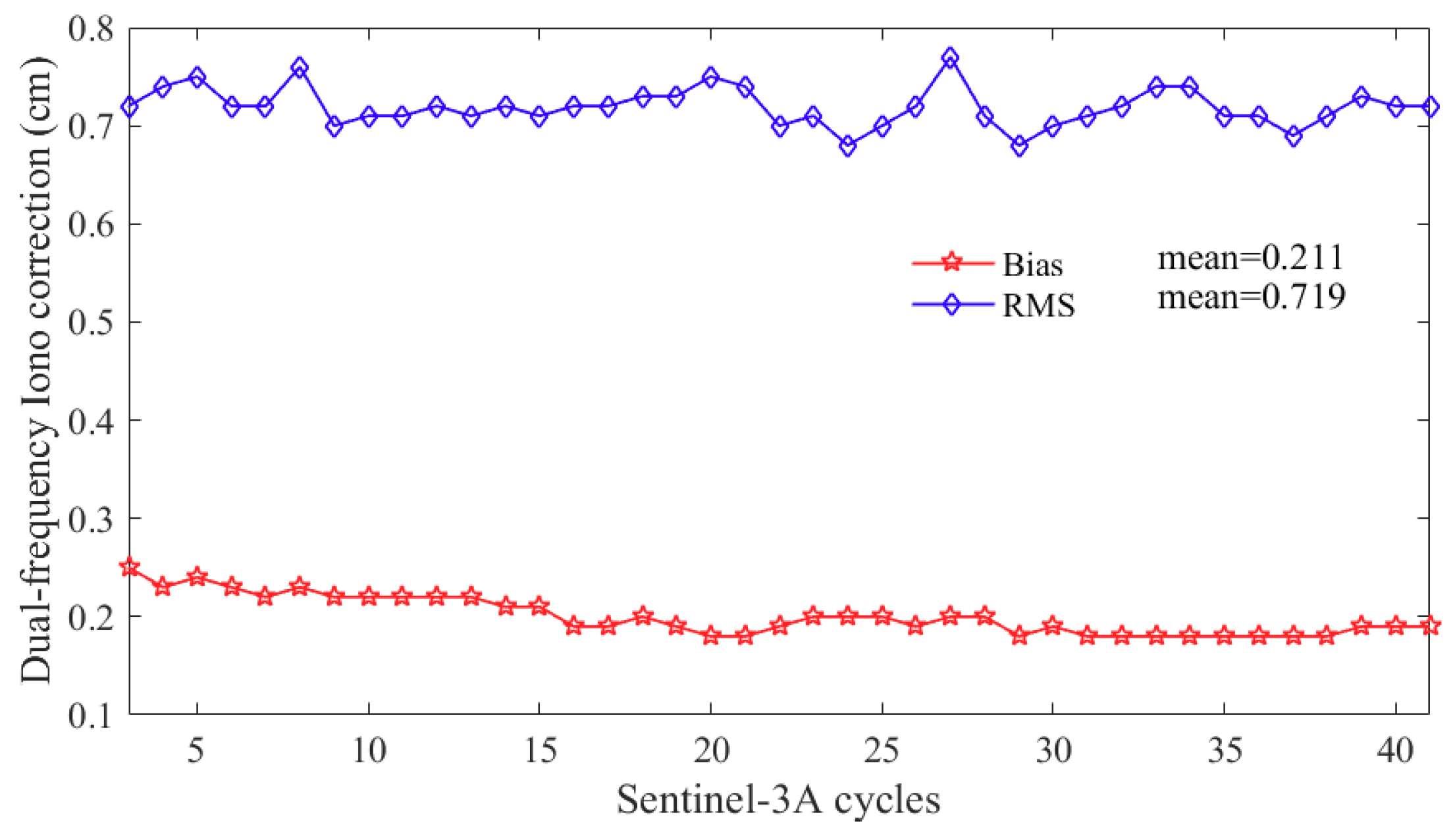
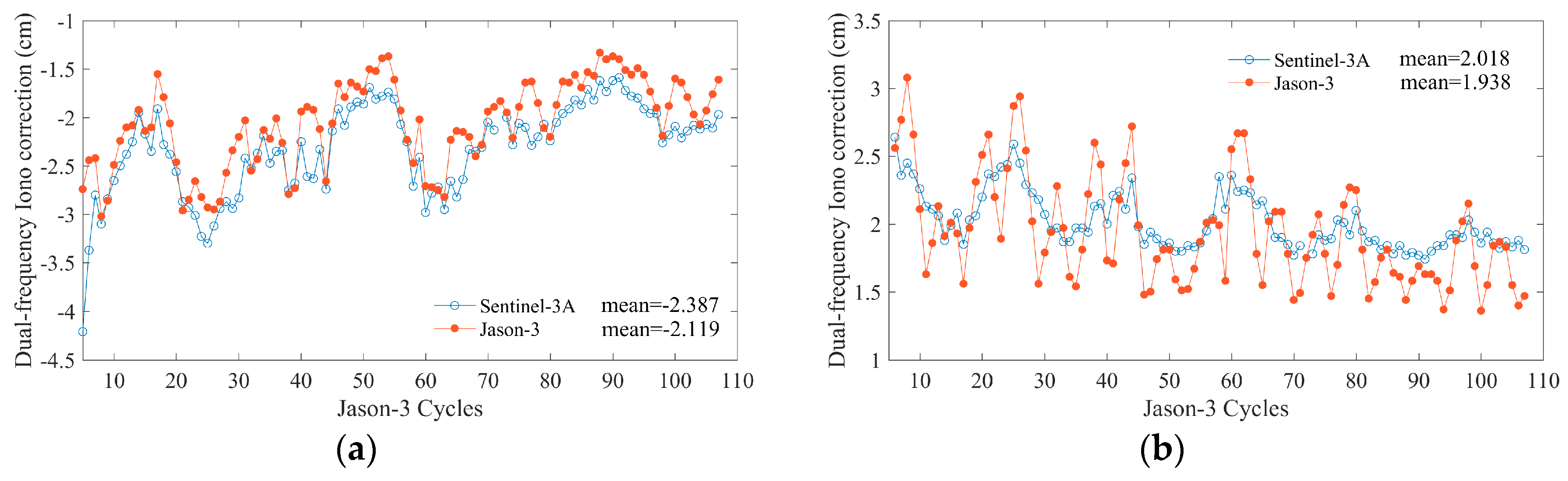
3.2.2. Ionospheric Correction

The ionospheric path delay is caused by the refraction of the altimeter pulse signal by free electrons in the atmosphere. Correction of ionospheric path delay is also critical for accurate altimetric estimation of the range from the satellite to the sea surface. The ionospheric path delay is generally corrected using the Global Ionosphere Maps (GIM) model or measurements from the dual frequency altimeter. Dual frequency ionospheric correction is the best solution. Three kinds of ionospheric corrections, including the GIM model, SAR mode dual frequency, and PLRM mode dual frequency, are compared and analyzed. The cycle by cycle means and standard deviations of ionospheric corrections based on Sentinel-3A repeat cycles are compared in Figure 6. The variations of means of ionospheric corrections have a slightly descending trend. The variations of standard deviations of ionospheric corrections have a period of about half a year. The variations of ionospheric corrections are relative to the free electron content in the atmosphere. The cycle by cycle biases and RMSEs of dual frequency ionospheric correction differences between SAR and PLRM mode are shown in Figure 7. The biases and RMSEs are stable. SAR mode dual frequency ionospheric correction has a systemic bias of 0.211 cm relative to PLRM mode. The variations of bias and RMSE have no trend, and this indicates the good performance of Sentinel-3A.

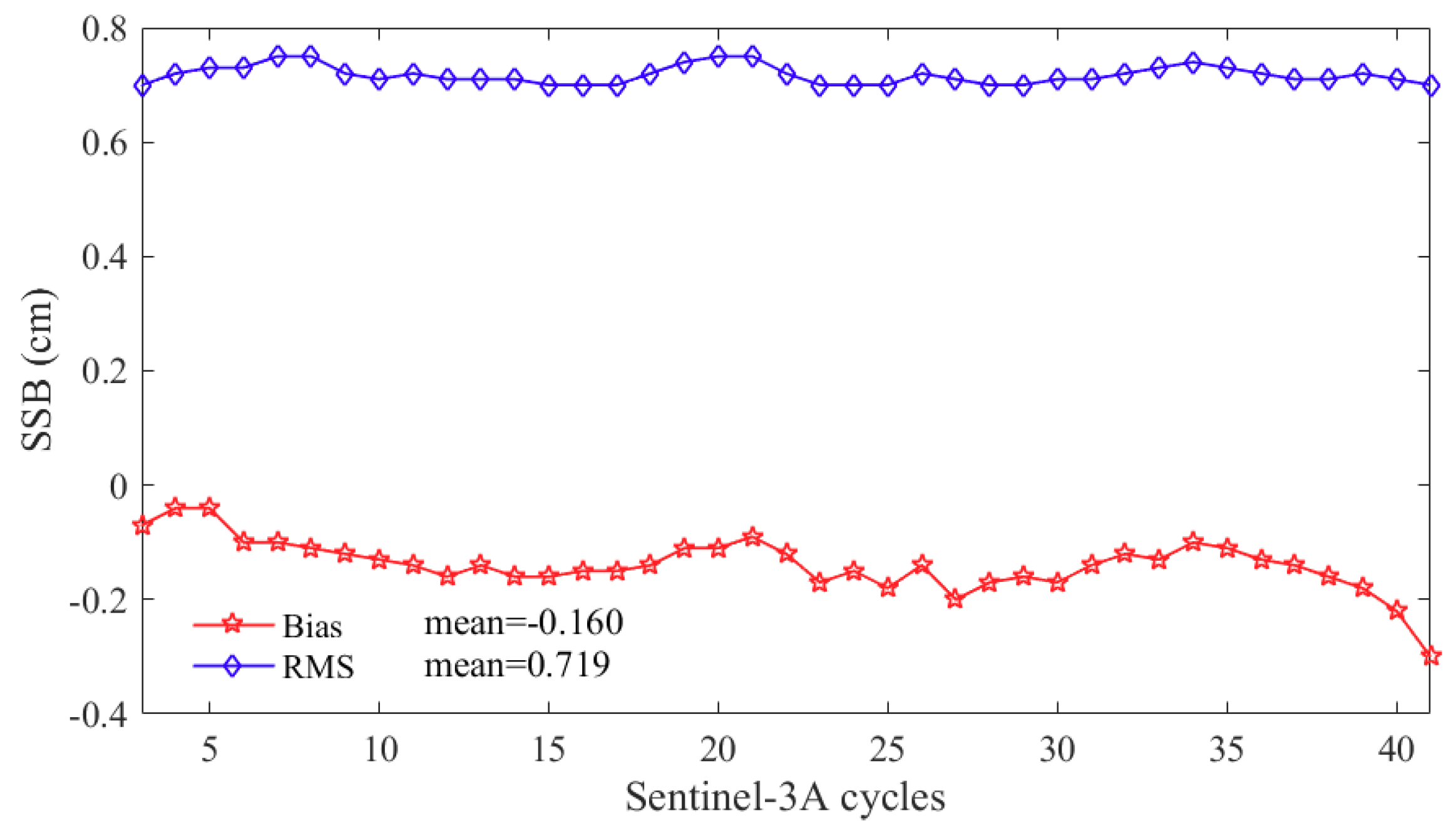
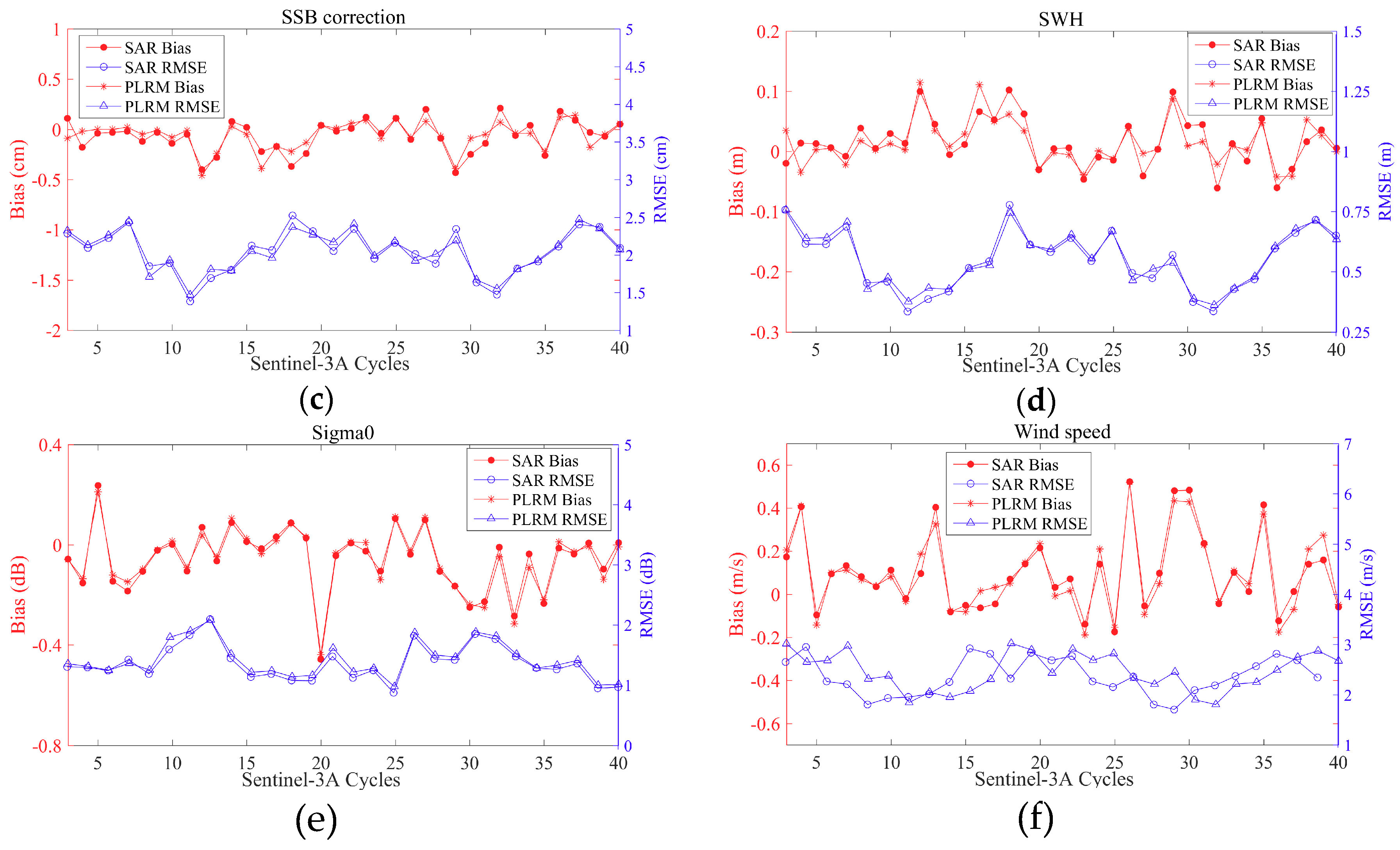
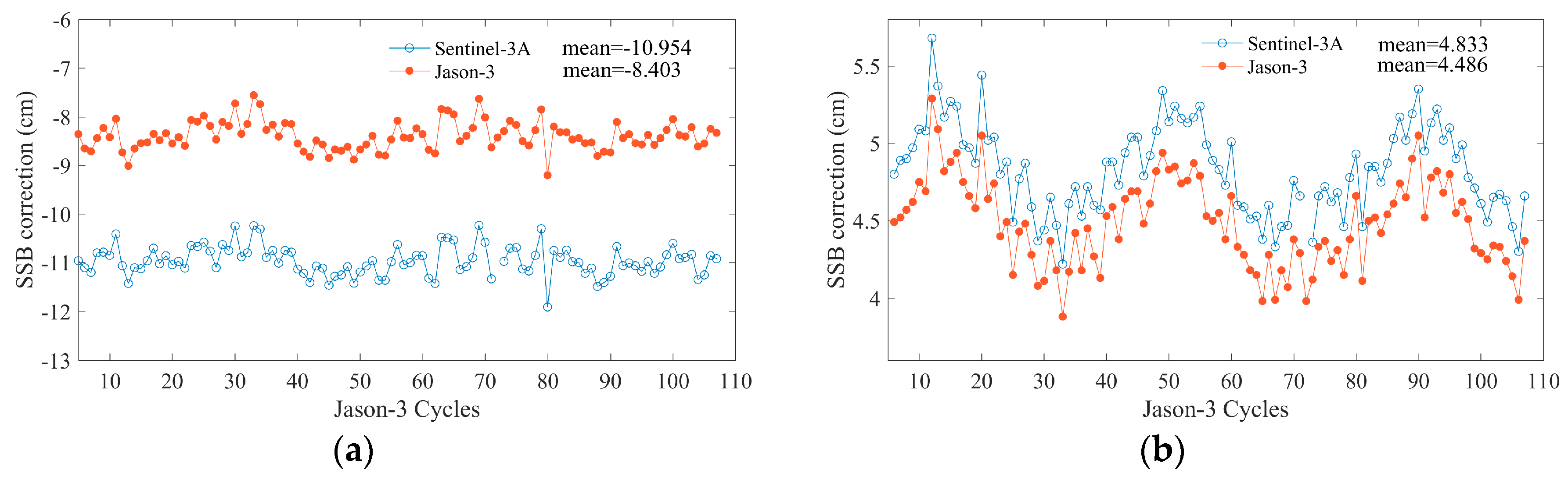
3.2.3. Sea State Bias (SSB) Correction

The shape of the altimeter return waveform is determined by the distribution of specular scatterers of small wave facets within the antenna footprint. The altimeter range measurements must be corrected for biases in the estimate of mean sea level that arise due to the distributions of the scatters and the sea surface height. This is sea state bias correction. SSB correction is related to SWH, and SWH measured by SRAL is used for SSB correction. The cycle by cycle means and standard deviations of SSB corrections according to Sentinel-3A repeat cycles are compared in Figure 8. The variations of means and standard deviation of SSB corrections with time have no trend. The variations of standard deviations of SSB corrections have a period of about a year. This shows the stability of SSB corrections with time. The cycle by cycle biases and RMSEs of SSB correction differences between SAR and PLRM mode are shown in Figure 9. The biases and RMSEs are stable and have no trend. SAR mode SSB correction has a systemic bias of 0.719 cm relative to PLRM mode.

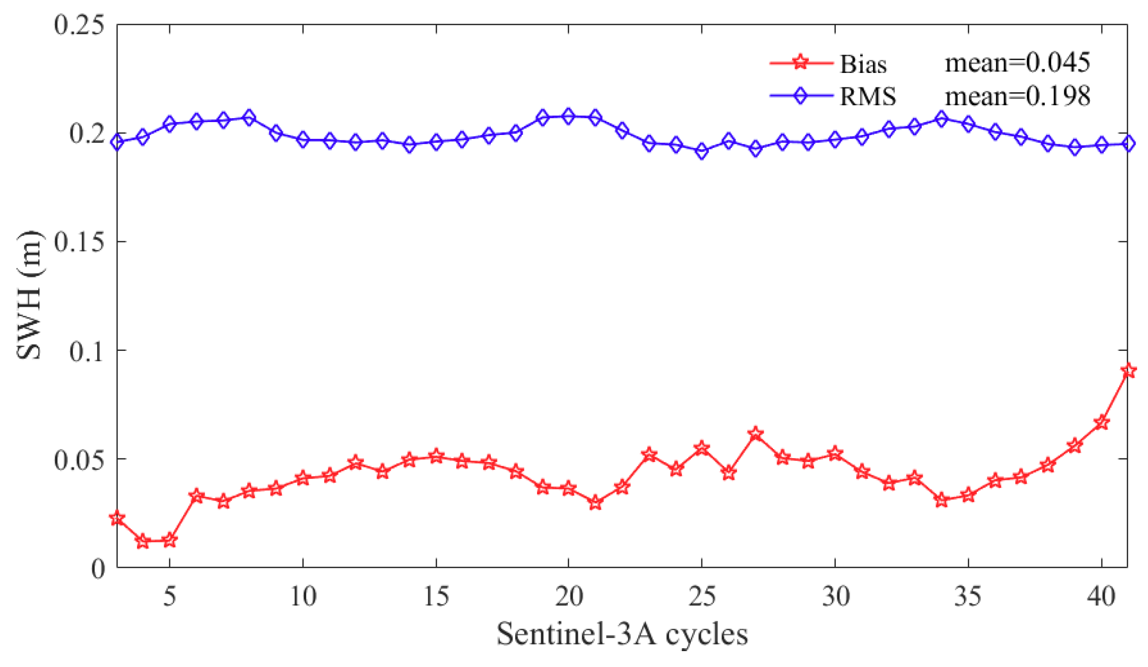
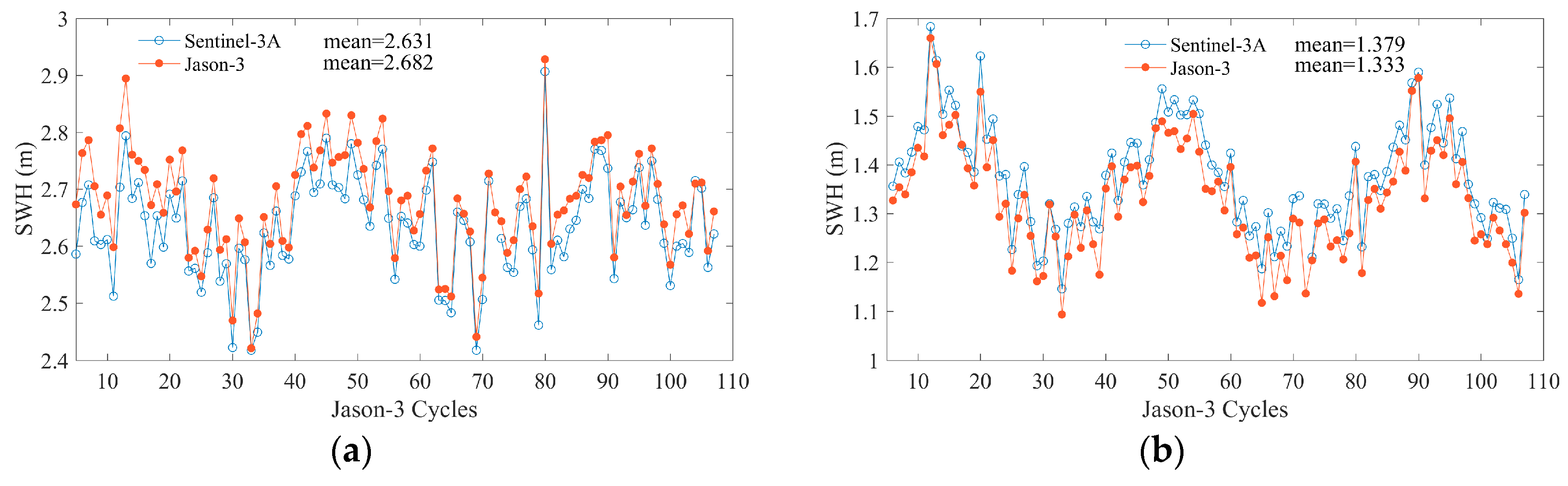
3.2.4. Significant Wave Height

Significant Wave Height (SWH) can be determined based on the slope of the altimeter return waveform. SWH is one of the most important measurement parameters carried out by the altimeter. The cycle by cycle means and standard deviations of SWHs according to Sentinel-3A repeat cycles are compared in Figure 10. The variations of standard deviations of SWHs have a period of about a year. This is related to the seasonal variations of the global ocean. The variations of the mean and standard deviation of the SWHs have no trend. The cycle by cycle biases and RMSEs of SWH differences between SAR and PLRM mode are shown in Figure 11. The biases and RMSEs of SWH differences are stable and the mean of the biases is less than 0.05 m. This means that there is a small difference between SAR and PLRM mode SWH, with a systemic bias of 0.045 m.

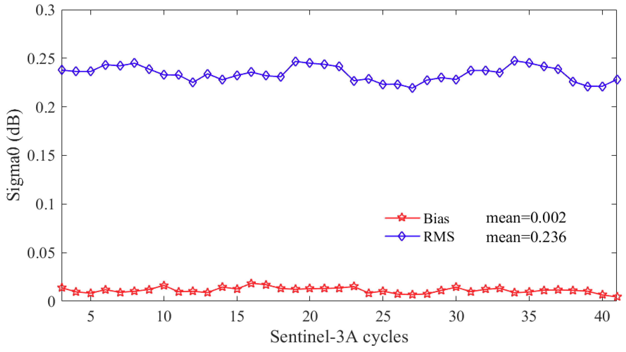
3.2.5. Backscattering Coefficient (Sigma0)
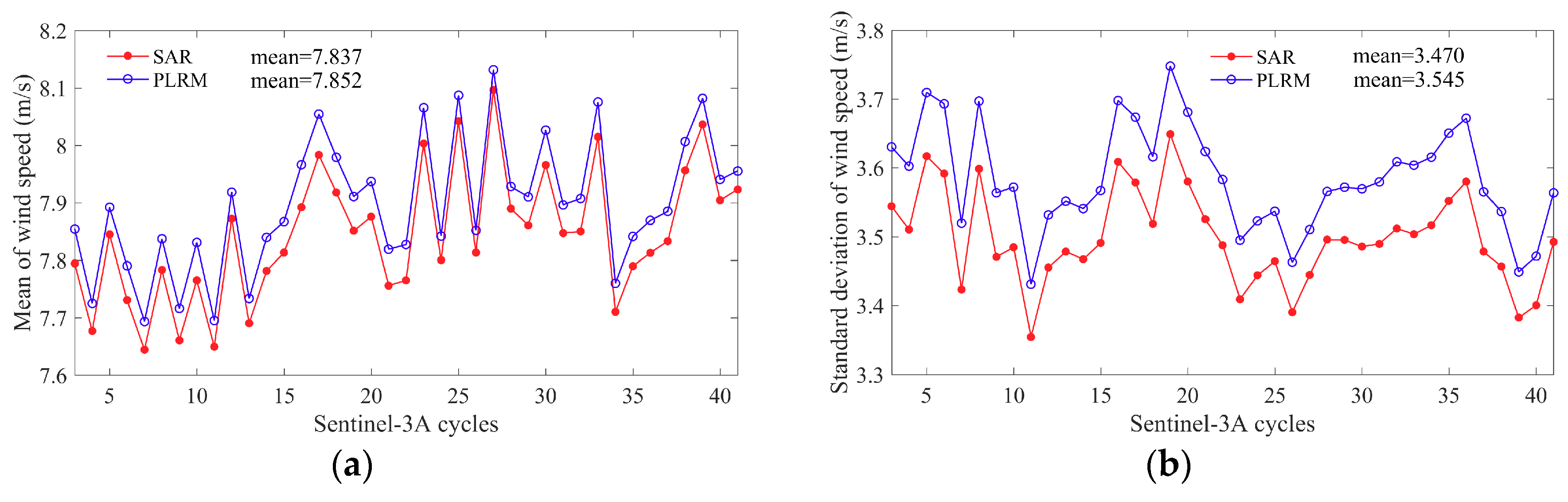
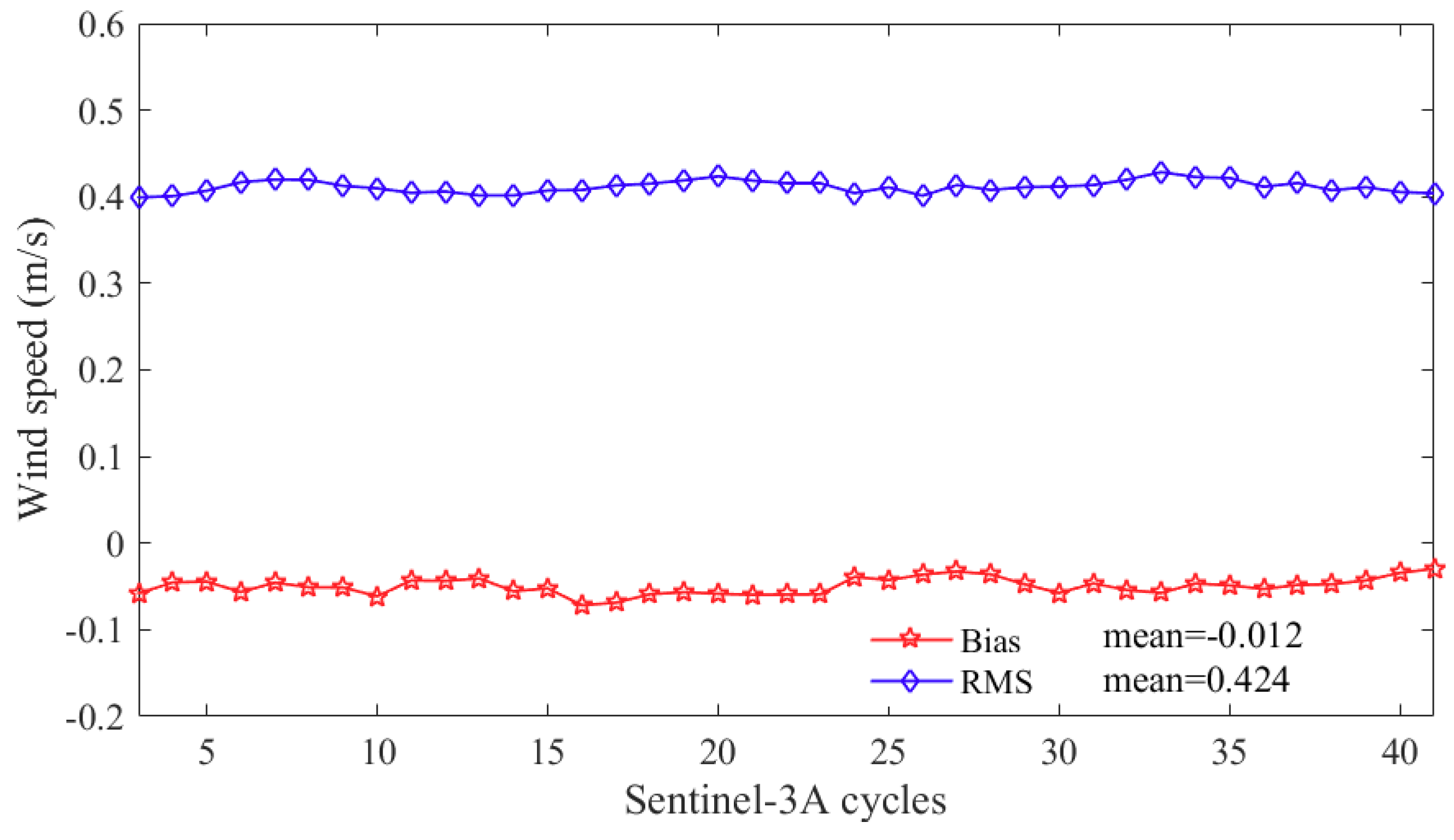
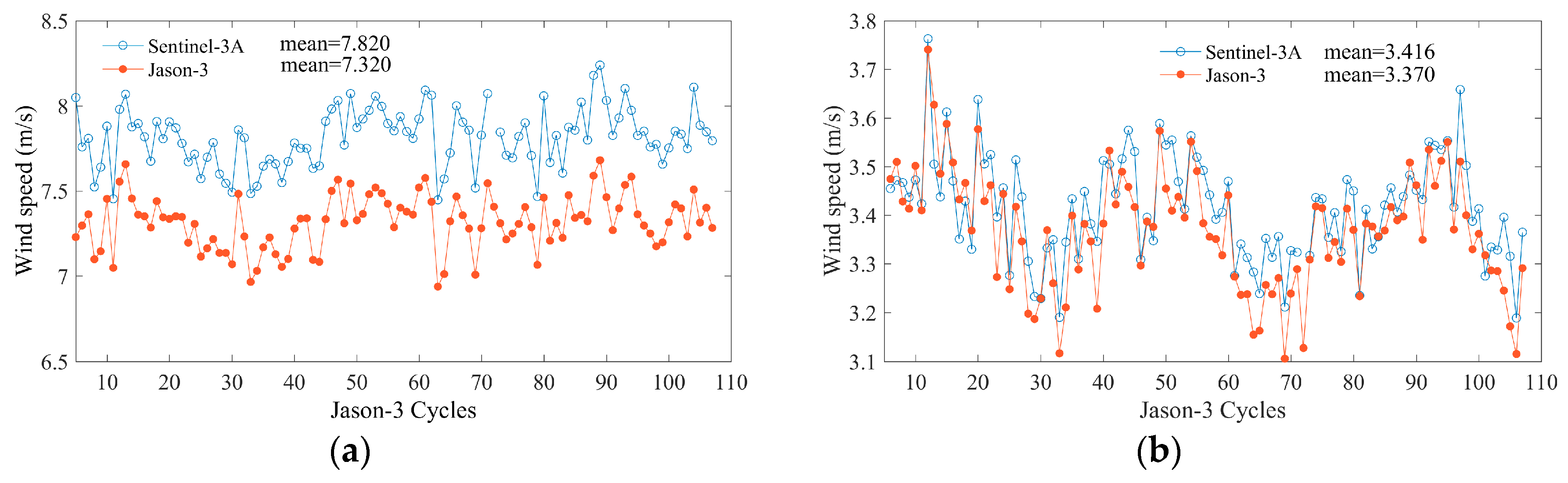
The amplitude of radar altimeter echo signals with respect to the emission amplitude gives the backscattering coefficient. The backscattering coefficient can be related to wind speed. Empirical models establish a relation between the wind speed, and the sea surface backscattering coefficient and significant wave height. The cycle by cycle means and standard deviations of backscattering coefficients according to Sentinel-3A repeat cycles are compared in Figure 12. The backscattering coefficients of SAR and PLRM mode are very consistent. The variations of means and standard deviations of backscattering coefficients have no obvious trend. The cycle by cycle biases and RMSEs of the differences in backscattering coefficient between SAR and PLRM modes are shown in Figure 13. The biases of backscattering coefficient differences are close to 0. The RMSEs of backscattering coefficient differences are less than 0.25 dB. The biases and RMSEs are stable and have no trend over time. This indicates the consistency of the backscattering coefficients between the SAR and PLRM modes.

3.2.6. Wind Speed

Wind speed is derived from the backscattering coefficient by the inversion model function. The cycle by cycle means and standard deviations of wind speed according to Sentinel-3A repeat cycles are compared in Figure 14. It can be seen that the wind speed of SAR and PLRM mode are very consistent. The variations of means and standard deviations of wind speeds have no trend and drift with time. The cycle by cycle biases and RMSEs of wind speed differences between SAR and PLRM mode are shown in Figure 15. The biases and RMSEs of wind speed differences are stable. The biases are close to 0, and the RMSEs are less than 0.5 m/s. This also proves the consistency of SAR and PLRM mode backscattering coefficient measurement.

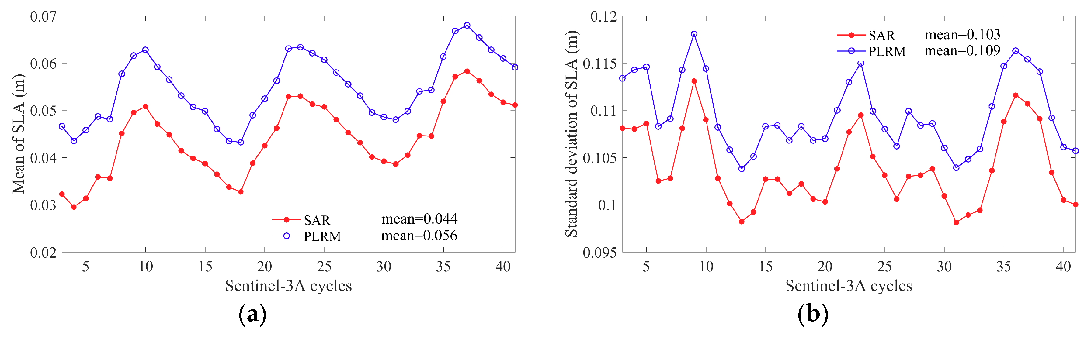
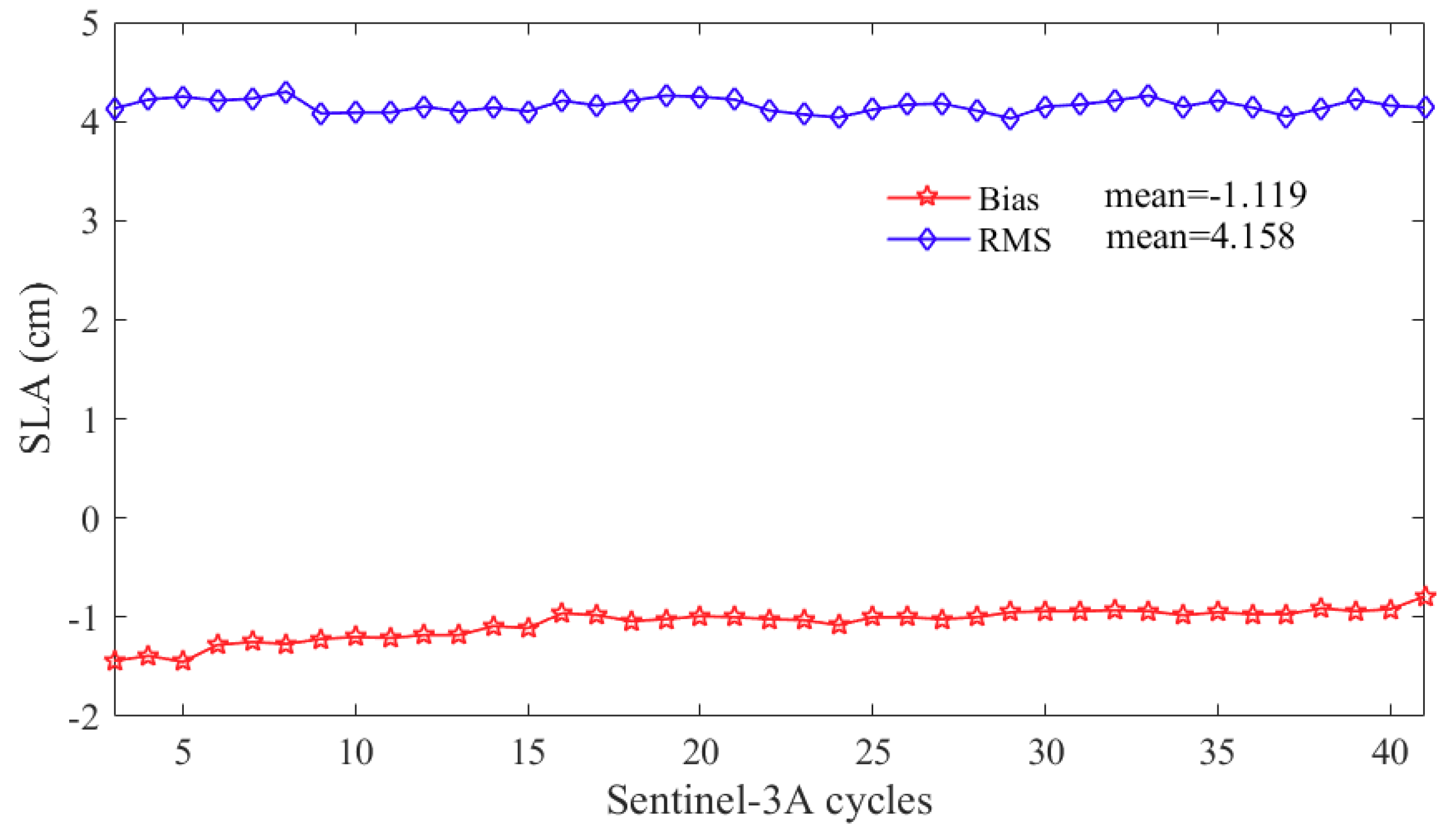
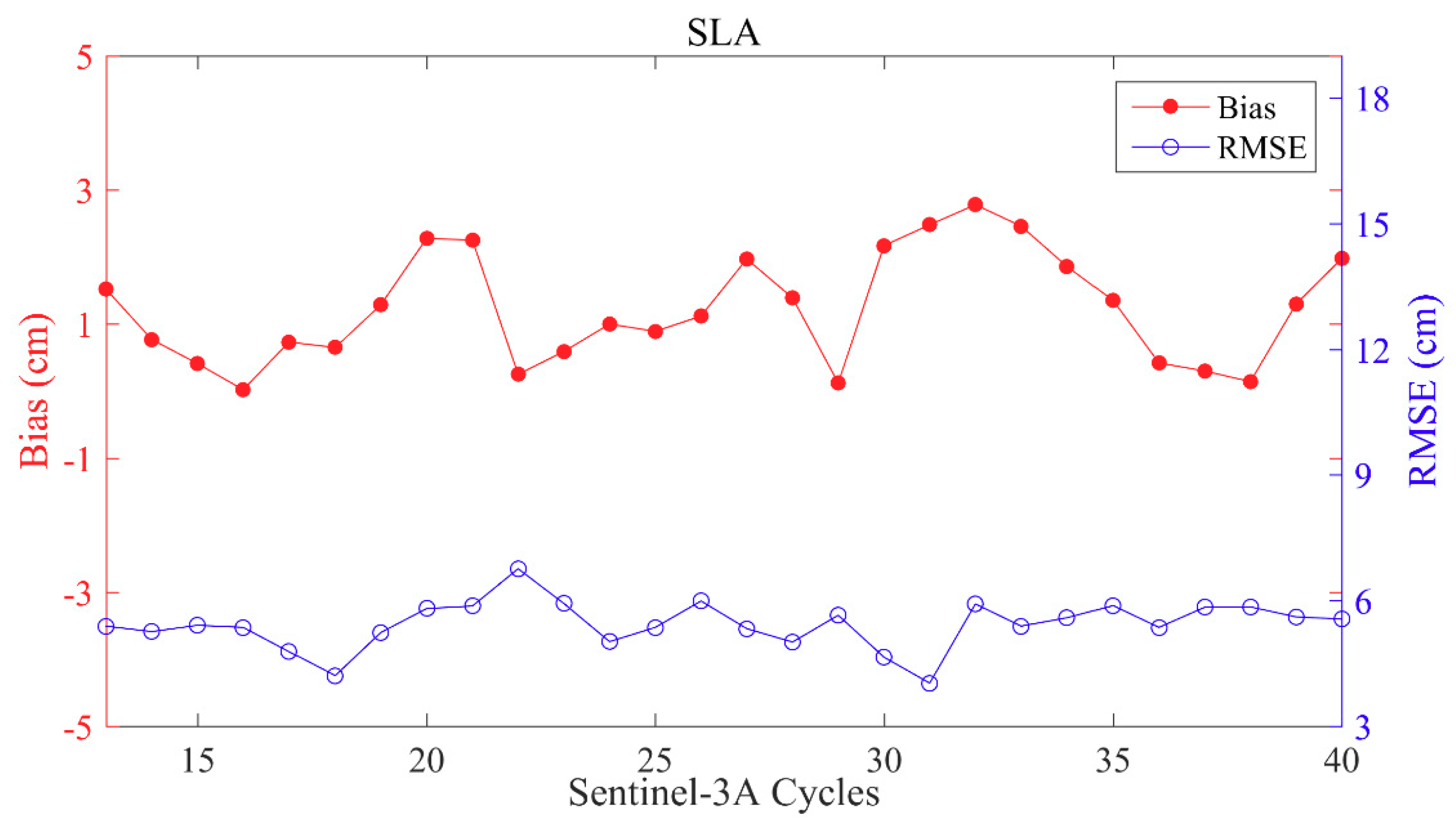
3.2.7. Sea Surface Height

Sea Surface Height (SSH) is one of the most important parameters measured by the altimeter. The range from the satellite to the sea surface can be measured by the altimeter. By combining the height of orbit, range corrections and geophysical corrections, the calculation of SSH is defined as follows:
SSH = Orbit Altimeter   Range c o r r e c t i o n s
where, corrections includes dry tropospheric correction, inverse barometer correction, radiometer wet tropospheric correction, dual frequency ionospheric correction, SSB correction, ocean tide correction, earth tide correction and pole tide correction. Sea level anomaly (SLA), defined as the difference between SSH and the mean sea surface (MSS), is the most important parameter of the altimeter used in scientific research. Therefore, the evaluation of SLA is used to validate SSH and the performance of the altimeter. The cycle by cycle means and standard deviations of the SLA of SAR and PLRM modes according to Sentinel-3A repeat cycles are presented in Figure 16. The means of SLA are less than 7 cm and have a slight ascending trend, which is related to the rising global sea level. The standard deviations of SLA have no trend over time. All these demonstrate the stability of SSH measurement by Sentinel-3A SRAL.
The cycle by cycle biases and RMSEs of SLA differences between SAR and PLRM mode are given in Figure 17. The absolute biases of SLA differences between SAR and PLRM mode are less than 1.12 cm, and the RMSEs are less than 5 cm. These results also prove the stability of Sentinel-3A SRAL SSH measurement.

3.3. Comparisons at Self-Crossovers

In theory, Sentinel-3A SRAL parameters at its self-crossovers with short measurement time differences should be consistent. Comparisons of these parameters at self-crossovers make it possible to evaluate the stability and accuracy of Sentinel-3A SRAL data. Self-crossovers are the ground track cross-points of different passes in the same cycle of Sentinel-3A. Sentinel-3A SRAL data, including radiometer wet tropospheric correction, dual frequency ionospheric correction, SSB correction, SWH, Sigma0 and wind speed, are compared within a measurement time difference of less than 9 h. The cycle by cycle biases and RMSEs of differences of these parameters are shown in Figure 18.
It can be seen in Figure 18 that the total cycle average biases of wet tropospheric correction, inonospheric correction, SSB correction and SWH differences are very close to 0, except that of backscattering coefficient (−0.04 dB) and wind speed (0.07 m/s). This demonstrates the stabilities of all Sentinel-3A parameters and performances. The total cycle average RMSEs of wet tropospheric correction differences, ionospheric correction differences and SSB correction differences are 1.6 cm, 1.9 cm and 2.1 cm, respectively. Good accuracies of these corrections ensure the good performance of Sentinel-3A SRAL SSH measurements. The total cycle average RMSE of SWH differences is less than 0.55 m [17]. Ocean waves change rapidly, and the self-crossover measurement time difference of 9 h causes large differences in SWH at the self-crossovers. The total cycle average RMSEs of backscattering coefficient and wind speed differences are 1.4 dB and 2.4 m/s, respectively. These are due to the rapid change in sea surface wind speed and the time difference of 9 h. The biases and RMSEs fluctuate slightly in different cycles and have no trend with time. This means that the performance of Sentinel-3A SRAL is stable and has good accuracy.
The SLA comparisons at the self-crossovers of Sentinel-3A SRAL with measurement time difference of less than 9 h are used to validate the performance of Sentinel-3A SRAL. The RMSEs of SLA differences conventionally provide an estimate of the overall performance of the altimeter system. The mean of self-crossover SLA differences represents the average of SLA differences between ascending and descending passes of Sentinel-3A SRAL. The cycle by cycle biases and RMSEs of SAR mode SLA differences at the self-crossovers is given in Figure 19. As shown in Figure 19, the total cycle average biases and RMSEs of SLA differences are 1.2 cm and 5.4 cm, respectively. This means that Sentinel-3A SRAL has good performance and accuracy for SSH measurement. The map of self-crossover SLA differences averaged over the whole mission is plotted in Figure 20. The SLA differences mainly range between -10 cm and 10 cm. The regions with large SLA differences are always high ocean variability areas such as equatorial current, Antarctic Circumpolar Current and high-latitude areas. This also proves that Sentinel-3A has good performance.

3.4. Comparisons with Jason-3

3.4.1. Cross-Calibration with Jason-3

Due to the high accuracy of Jason-3 data, the radiometer wet tropospheric correction, dual frequency ionospheric correction, SSB correction, SWH, Sigma0, wind speed and SLA of Sentinel-3A SRAL are compared with those of Jason-3 at their dual-crossovers based on measurement time differences of 30 min. Dual-crossovers are the ground track cross-points between passes of Sentinel-3A and Jason-3. The cycle by cycle biases and RMSEs of these parameter differences at the dual-crossovers are shown in Figure 21 and Figure 22.
As shown in Figure 21, the total cycle average bias and RMSE of radiometer wet tropospheric correction differences are −0.69 cm and 0.67 cm. The total cycle average bias and RMSE of dual frequency ionospheric differences are −0.42 cm and 1.66 cm. The total cycle average bias and RMSE of SSB correction differences are −2.86 cm and 0.8 cm. The biases and RMSEs of radiometer wet tropospheric correction, dual frequency ionospheric correction and SSB correction differences fluctuate slightly and have no trend with time. These results prove the stabilities of the corrections and the good performance of radiometer and SRAL measurement. The total cycle average bias and RMSE of SWH differences are 0.039 m and 0.203 m for SAR mode SWH and −0.037 m and 0.211 m for PLRM mode SWH. The small biases and the RMSEs of less than 0.25 m show good performance of Sentinel-3A SRAL SWH measurement. The total cycle average bias and RMSE of backscattering coefficient differences is −2.84 dB and 0.33 dB. The total cycle average bias and RMSE of wind speed differences is 0.69 m/s and 0.72 m/s. These results demonstrate that the performance of Sentinel-3A SRAL wind speed measurement is as good as that of Jason-3.
Like the comparisons of other parameters, SAR mode SLA of Sentinel-3A are compared to SLA of Jason-3 at their dual-crossovers with measurement time differences of less than 30 min in order to evaluate the performance of Sentinel-3A SRAL SSH measurement. The bias of SLA differences at dual-crossovers represents the average SLA differences between Sentinel-3A SRAL and Jason-3. The total cycle average bias and RMSE of SLA differences are 2.96 cm and 4.67 cm. These results show the consistency between Sentinel-3A and Jason-3, and that the performance of the Sentinel-3A SRAL SSH measurements are as good as those of Jason-3.

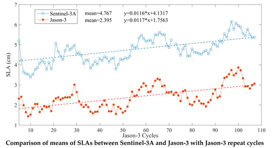
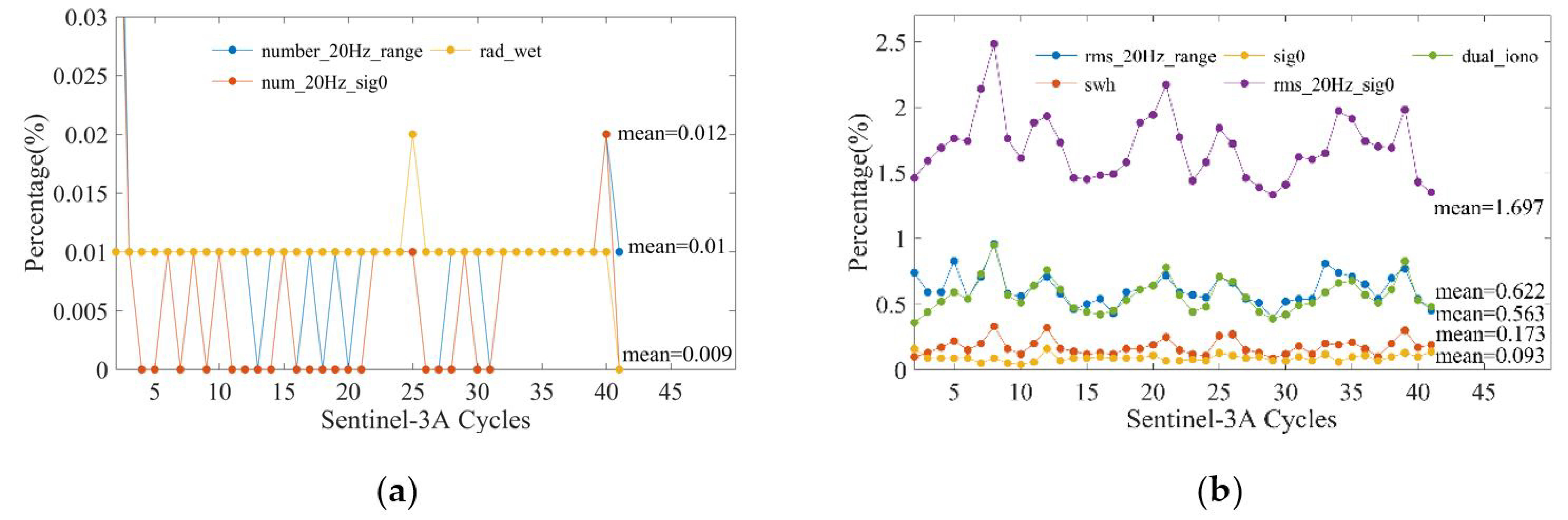
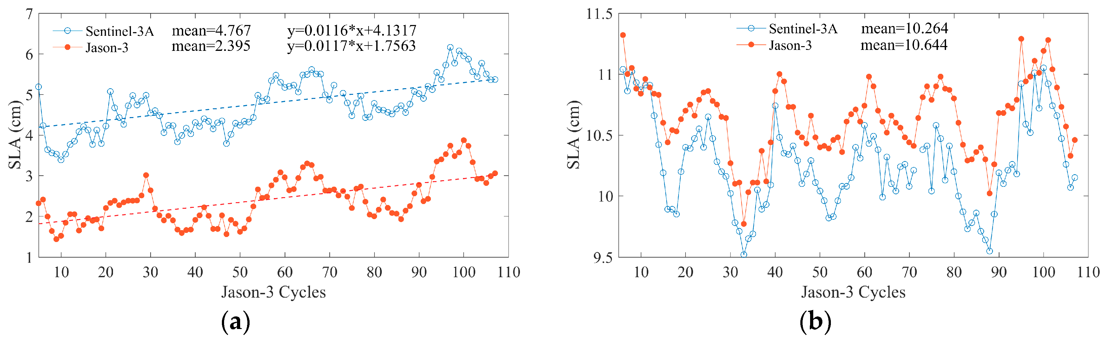
3.4.2. Cycle by Cycle Statistical Analysis on Jason-3 Cycle

Because the spatial coverage of Sentinel-3A is larger than Jason-3, the data of Sentinel-3A SRAL is limited to the same spatial coverage area as Jason-3 (between 66°N and 66°S) for this comparison. Sentinel-3A SRAL data are divided into different subsets according to Jason-3 cycles. Sentinel-3A data from the same time period as the Jason-3 cycle of 10 days forms one subset. The cycle by cycle means and standard deviations of these limited Sentinel-3A and Jason-3 data are calculated and compared. The cycle by cycle means and standard deviations of radiometer wet tropospheric corrections, dual ionospheric corrections, SSB corrections, SWHs, backscattering coefficients and wind speeds of Sentinel-3A and Jason-3 according to Jason-3 repeat cycles are compared in Figure 23, Figure 24, Figure 25, Figure 26, Figure 27 and Figure 28.
The differences in mean and standard deviation of radiometer wet tropospheric corrections between Sentinel-3A and Jason-3 are about 0.017 m and 0.046 m. They are almost equal, with the same variations. It is shown that the performance of the radiometer wet tropospheric corrections of Sentinel-3A is similar to that of Jason-3. The differences in the mean and standard deviation of dual frequency ionospheric corrections are about 0.268 cm and 0.08 cm. The slight fluctuations of RMSEs show that the dual frequency ionospheric correction of Sentinel-3A is more stable than Jason-3. This means that the performance of the dual frequency ionospheric correction of Sentinel-3A is better than Jason-3. The differences in the mean and standard deviation of SSB corrections are about 2.65 cm and 0.35 cm. The fluctuations of RMSEs of Sentinel-3A are similar to those of Jason-3. This means the performance of SSB correction is consistent with that of Jason-3. The differences in mean and standard deviation of SWHs are about 0.66 m and 0.046 m. This is due to the different spatial coverage between Sentinel-3A and Jason-3. The small difference in standard deviation means that the SWH of Sentinel-3A has the same accuracy as Jason-3. All these results mean that the performance of SWH measurement is consistent with Jason-3. The differences in the total mean show that the backscattering coefficients of Sentinel-3A SRAL have a systemic bias of about 3 dB compared with those of Jason-3. The differences in mean and standard deviation between the backscattering coefficients are about 2.76 dB and 0.10 dB. This demonstrates the consistency of the backscattering coefficients between Sentinel-3A SRAL and Jason-3. The differences in mean and standard deviation of wind speed are about 0.5 m/s and 0.046 m/s. This means that wind speeds between Sentinel-3A and Jason-3 have a small difference, arising from their different spatial coverages, and it also proves the consistency of the data accuracy of wind speed between Sentinel-3A SRAL and Jason-3. All of the above comparisons between Sentinel-3A and Jason-3 show consistency and accuracies as good for Sentinel-3A as they are for Jason-3.
Apart from the dual-crossover comparisons, Sentinel-3A SRAL SAR mode SLA is compared to Jason-3 with the same global coverage and time period for the evaluation of Sentinel-3A SLA global distribution. Ignoring the differences in geophysical corrections for Sentinel-3A SRAL and Jason-3, cycle by cycle means and standard deviations of SLAs with a global coverage between 66°S and 66°N are calculated in the period of Jason-3 repeat cycles as shown in Figure 29. The differences of mean and standard deviation of SLAs between Sentinel-3A and Jason-3 are about 2.47 cm and 0.38 cm. This means SSH measurement of Sentinel-3A has a systemic bias of about 2.5 cm relative to SSH measurement of Jason-3. The variations of means of SLA between Sentinel-3A and Jason-3 are similar and have the same ascending trend (as shown in Figure 29a) corresponding to the rise in global sea level. Their standard deviations are also similar, and their total average difference is less than 1 cm. These results show that good performance of Sentinel-3A SRAL SSH measurement is as that of Jason-3.

4. Conclusions

In this paper, the data quality of Sentinel-3A SRAL is assessed and the performance of SRAL is estimated by verifying the data availability and monitoring the parameters of the altimeter and radiometer, which include wet tropospheric correction, ionospheric correction, Sea State Bias (SSB) correction, Significant Wave Height (SWH), backscattering coefficient (Sigma0), wind speed and Sea Surface Height (SSH) (Sea Level Anomaly (SLA) is always used in oceanography study), through global statistical analysis of Sentinel-3A data and comparison at self-crossovers, as well as comparisons with the Jason-3 mission.
The results of data verification show that Sentinel-3A SRAL, which has a larger number of 20 Hz range measurements and a smaller standard deviation of 20 Hz range measurements relative to Jason-3, has better measurement performance and data availability than Jason-3. The cycle by cycle global statistical analysis of Sentinel-3A SRAL data according to Sentinel-3A cycles showed the good performance and data stability of Sentinel-3A SRAL data. The results showed that the parameters of the SAR and PLRM modes had very small differences. The mean biases of radiometer wet tropospheric correction, dual frequency ionospheric correction, SSB correction, SWH, Sigma0 and wind speed between SAR and PLRM mode were −0.006 cm, 0.211 cm, −0.16 cm, 0.045 cm, 0.002 dB and 0.012 m/s, respectively. Comparisons at the self-crossovers and cross-calibration with Jason-3 show the performance stabilities and high accuracy of parameters, and their variations have no trend with time. The global statistical analysis of parameters between Sentinel-3A and Jason-3 according to Jason-3 repeat cycles show the consistencies of Sentinel-3A and Jason-3, and there are only small systemic biases of parameters between Sentinel-3A and Jason-3. The absolute systemic biases of radiometer wet tropospheric correction, dual frequency ionospheric correction, SSB correction, SWH, Sigma0 and wind speed between Sentinel-3A and Jason-3 were no more than 0.69 cm, 0.42 cm, 2.86 cm, 0.04 m, 2.84 dB and 0.69 m/s, respectively. With respect to the analysis of sea surface height (SSH), the mean bias of SLA between SAR and PLRM mode was about 1 cm. Cross-calibration with Jason-3 showed that the total cycle average RMSE of SLA difference was about 4.67 cm. The systemic bias of SLA between Sentinel-3A and Jason-3 was about 2.96 cm. In general, the global statistical analysis of the parameters of SRAL and the radiometer demonstrate the performance stabilities of these parameters, and the variations of the parameters have no trend with time. The results show that Sentinel-3A has very good performance and data accuracy. Sentinel-3A is a new kind of altimetry data for the global ocean studies and operational ocean forecasting.

Author Contributions

Conceptualization, J.Y. and J.Z.; methodology, J.Y.; validation, J.Y. and C.W.; formal analysis, J.Y.; writing—original draft preparation, J.Y.; writing—review and editing, J.Y. and C.W.; visualization, J.Y. and C.W.

Funding

This research was funded by National Key R and D Program of China (grant number 2016YFC1401800), the National Natural Science Foundation of China (41576176) and Dragon 4 Project (ID.32292).

Acknowledgments

The authors would like to thank the EUMETSAT for Sentinel-3A/3B data, the CNES AVISO for Jason-3 data.

Conflicts of Interest

The authors declare no conflict of interest.

References

  1. Donlon, C.; Berruti, B.; Buongiorno, A.; Ferreira, M.H.; Femenias, P.; Frerick, J.; Goryl, P.; Klein, U.; Laur, H.; Mavrocordatos, C.; et al. The Global Monitoring for Environment and Security (GMES) Sentinel-3 mission. Remote Sens. Environ. 2012, 120, 37–57. [Google Scholar] [CrossRef]
  2. Le Roy, Y.; Deschaux-Beaume, M.; Mavrocordatos, C.; Aguirre, M.; Heliere, F. SRAL SAR radar altimeter for sentinel-3 mission. In Proceedings of the 2007 IEEE International Geoscience and Remote Sensing Symposium, Barcelona, Spain, 23–28 July 2007. [Google Scholar]
  3. Le Roy, Y.; Deschaux-Beaume, M.; Mavrocordatos, C.; Borde, F. SRAL, A radar altimeter designed to measure a wide range of surface types. In Proceedings of the 2009 IEEE International Geoscience and Remote Sensing Symposium, Cape Town, South Africa, 12–17 July 2009. [Google Scholar] [CrossRef]
  4. Mitchum, G.T. Monitoring the Stability of Satellite Altimeters with Tide Gauges. J. Atmos. Ocean. Technol. 1998, 15, 721–730. [Google Scholar] [CrossRef]
  5. Vincent, P.; Desai, S.D.; Dorandeu, J.; Ablain, M.; Soussi, B.; Callahan, P.S.; Haines, B.J. Jason-1 Geophysical Performance Evaluation. Mar. Geod. 2003, 26, 167–186. [Google Scholar] [CrossRef]
  6. Perbos, J.; Escudier, P.; Parisot, F.; Zaouche, G.; Vincent, P.; Menard, Y.; Manon, F.; Kunstmann, G.; Royer, D.; Fu, L.L. Jason-1: Assessement of the System Performances. Mar. Geod. 2003, 26, 147–157. [Google Scholar] [CrossRef]
  7. Dorandeu, J.; Ablain, M.; Faugere, Y.; Mertz, F.; Soussi, B.; Vincent, P. Jason-1 global statistical evaluation and performance assessment: Calibration and cross-calibration results. Mar. Geod. 2004, 27, 345–372. [Google Scholar] [CrossRef]
  8. Ablain, M.; Philipps, S.; Picot, N.; Bronner, E. Jason-2 Global Statistical Assessment and Cross-Calibration with Jason-1. Mar. Geod. 2010, 33, 162–185. [Google Scholar] [CrossRef]
  9. Ablain, M.; Philipps, S.; Thibaut, P.; Picot, N.; Lombard, A. Global Quality Assessment of Jason-2 measurements and consistency with Jason-1. In Proceedings of the AGU 2008 Fall Meeting, San Francisco, CA, USA, 15–19 December 2008. [Google Scholar]
  10. Faugere, Y.; Dorandeu, J.; Lefevre, F.; Picot, N.; Femenias, P. Envisat Ocean Altimetry Performance Assessment and Cross-calibration. Sensors 2006, 6, 100–130. [Google Scholar] [CrossRef] [Green Version]
  11. Prandi, P.; Philipps, S.; Pignot, V.; Picot, N. SARAL/AltiKa Global Statistical Assessment and Cross-Calibration with Jason-2. Mar. Geod. 2015, 38, 297–312. [Google Scholar] [CrossRef]
  12. Dettmering, D.; Schwatke, C.; Bosch, W. Global Calibration of SARAL/AltiKa Using Multi-Mission Sea Surface Height Crossovers. Mar. Geod. 2015, 38, 206–218. [Google Scholar] [CrossRef]
  13. Data Product Quality Reports. Available online: https://sentinel.esa.int/web/sentinel/technical-guides/sentinel-3-altimetry/data-quality-reports (accessed on 15 May 2019).
  14. Jason-3 GDR Quality Assessment Report Cycle 094 (SALP-RP-JALT3-EX-23103-CLS094). Available online: ftp://avisoftp.cnes.fr/Niveau0/AVISO/pub/jason-3/gdr_d_validation_report (accessed on 13 June 2019).
  15. Sentinel-3 SRAL Marine User Handbook (EUM/OPS-SEN3/MAN/17/920901, v1A e-signed). Available online: https://www.eumetsat.int/website/wcm/idc/idcplg?IdcService=GET_FILE&dDocName=PDF_S3_SRAL_HANDBOOK&RevisionSelectionMethod=LatestReleased&Rendition=Web (accessed on 5 May 2019).
  16. Gao, B.; Chan, P.K.; Li, R. A global water vapor data set obtained by merging the SSMI and MODIS data. Geophys. Res. Lett. 2004, 31. [Google Scholar] [CrossRef]
  17. Yang, J.G.; Zhang, J. Validation of Sentinel-3A/3B Satellite Altimetry Wave Heights with Buoys and Jason-3 Data. Sensors 2019, 19, 2914. [Google Scholar] [CrossRef]
Figure 1. The spatial distribution of self-crossovers of Sentinel-3A (blue) and dual-crossovers between Sentinel-3A and Jason-3 (red).
Remotesensing 11 01573 g001
Figure 2. Cycle by cycle percentages of rejected measurement by Sentinel-3A SRAL by the thresholds of (a) number of 20 Hz range measurements, number of 20 Hz Sigma0 measurements and radiometer wet tropospheric correction, and (b) RMS of 20 Hz range measurements, RMS of 20 Hz Sigma0 measurements, dual frequency ionospheric correction, Sigma0 and SWH during cycle 3–41.
Remotesensing 11 01573 g002
Figure 3. Cycle by cycle mean of (a) number and (b) RMS of 20 Hz range measurements according to Jason-3 repeat cycles.
Remotesensing 11 01573 g003
Figure 4. Cycle by cycle (a) means and (b) standard deviations of wet tropospheric corrections according to Sentinel-3A repeat cycles.
Remotesensing 11 01573 g004
Figure 5. Cycle by cycle biases and RMSEs of differences of wet tropospheric correction between SAR and PLRM mode.
Remotesensing 11 01573 g005
Figure 6. Cycle by cycle (a) means and (b) standard deviations of ionospheric corrections according to Sentinel-3A repeat cycles.
Remotesensing 11 01573 g006
Figure 7. Cycle by cycle biases and RMSEs of differences of dual frequency ionospheric correction between SAR and PLRM mode.
Remotesensing 11 01573 g007
Figure 8. Cycle by cycle (a) means and (b) standard deviations of SSB corrections according to Sentinel-3A repeat cycles.
Remotesensing 11 01573 g008
Figure 9. Cycle by cycle biases and RMSEs of differences of SSB correction between SAR and PLRM mode.
Remotesensing 11 01573 g009
Figure 10. Cycle by cycle (a) means and (b) standard deviations of SWHs according to Sentinel-3A repeat cycles.
Remotesensing 11 01573 g010
Figure 11. Cycle by cycle biases and RMSEs of SWH differences between SAR and PLRM mode.
Remotesensing 11 01573 g011
Figure 12. Cycle by cycle (a) means and (b) standard deviations of backscattering coefficients according to Sentinel-3A repeat cycles.
Remotesensing 11 01573 g012
Figure 13. Cycle by cycle biases and RMSEs of differences of backscattering coefficients between SAR and PLRM mode.
Remotesensing 11 01573 g013
Figure 14. Cycle by cycle (a) means and (b) standard deviations of wind speeds according to Sentinel-3A repeat cycles.
Remotesensing 11 01573 g014
Figure 15. Cycle by cycle biases and RMSEs of wind speed differences between SAR and PLRM mode.
Remotesensing 11 01573 g015
Figure 16. Cycle by cycle (a) means and (b) standard deviations of SLA according to Sentinel-3A repeat cycles.
Remotesensing 11 01573 g016
Figure 17. Cycle by cycle biases and standard deviations of SLA differences between SAR and PLRM mode.
Remotesensing 11 01573 g017
Figure 18. Cycle by cycle biases and RMSEs of differences of (a) radiometer wet tropospheric correction, (b) dual frequency ionospheric correction, (c) SSB correction, (d) SWH, (e) Sigma0 and (f) wind speed at the self-crossovers of Sentinel-3A
Remotesensing 11 01573 g018aRemotesensing 11 01573 g018b
Figure 19. Cycle by cycle biases and RMSEs of SAR mode SLA differences at the self-crossovers of Sentinel-3A.
Remotesensing 11 01573 g019
Figure 20. Map of Sentinel-3A SRAL SAR mode SLA differences at the self-crossovers.
Remotesensing 11 01573 g020
Figure 21. Cycle by cycle biases and RMSEs of (a) radiometer wet tropospheric correction, (b) dual frequency ionospheric correction, (c) SSB correction, (d) SWH, (e) backscattering coefficient, and (f) wind speed differences at dual-crossovers between Sentinel-3A and Jason-3 with measurement time difference of 30 min.
Remotesensing 11 01573 g021
Figure 22. Cycle by cycle biases and RMSEs of SLA differences at dual-crossovers between Sentinel-3A and Jason-3 with measurement time difference of 30 min.
Remotesensing 11 01573 g022
Figure 23. Comparison of cycle by cycle (a) means and (b) standard deviations of radiometer wet tropospheric corrections between Sentinel-3A and Jason-3 according to Jason-3 repeat cycles.
Remotesensing 11 01573 g023
Figure 24. Comparison of cycle by cycle (a) means and (b) standard deviations of dual frequency ionospheric corrections between Sentinel-3A and Jason-3 according to Jason-3 repeat cycles.
Remotesensing 11 01573 g024
Figure 25. Comparison of cycle by cycle (a) means and (b) standard deviations of SSB corrections between Sentinel-3A and Jason-3 according to Jason-3 repeat cycles.
Remotesensing 11 01573 g025
Figure 26. Comparison of cycle by cycle (a) means and (b) standard deviations of SWHs between Sentinel-3A and Jason-3 according to Jason-3 repeat cycles.
Remotesensing 11 01573 g026
Figure 27. Comparison of cycle by cycle (a) means and (b) standard deviations of backscattering coefficients between Sentinel-3A and Jason-3 according to Jason-3 repeat cycles.
Remotesensing 11 01573 g027
Figure 28. Comparison of cycle by cycle (a) means and (b) standard deviations of wind speeds between Sentinel-3A and Jason-3 with Jason-3 repeat cycles.
Remotesensing 11 01573 g028
Figure 29. Comparison of cycle by cycle (a) means and (b) standard deviations of SLAs between Sentinel-3A and Jason-3 with Jason-3 repeat cycles.
Remotesensing 11 01573 g029
Table 1. Technical characteristics of the Sentinel-3A SRAL instrument.
ParameterKu BandC Band
Frequency13.575 GHz5.41 GHz
Bandwidth350 MHz320 MHz
Tracking modesClosed loop and open loop
LRM pulse repetition frequency1920 Hz
SAR mode pulse repetition frequency18 kHz
SAR along track solution~300 m
Table 2. Thresholds used for the main altimeter and radiometer parameters in the Sentinel-3A SRAL data editing procedures.
ParameterMinimumMaximum
Orbit-Range−130 m100 m
Sea level Anomaly−2 m2 m
Number of 20 Hz range measurements10-
Standard deviation of 20 Hz range measurements0 m0.2 m
Dry tropospheric correction−2.5 m−1.9 m
Wet tropospheric correction−0.5 m−0.001 m
Dual frequency ionosphere correction−0.4 m0.04 m
Sea state bias correction−0.5 m0 m
Backscattering coefficient5.0 dB28.0 dB
Standard deviation of 20 Hz Sigma0 measurements0 dB0.7 dB
Number of 20 Hz Sigma0 measurements10-
Significant wave height0 m11 m
Wind speed0 m/s30 m/s
Ocean tide−5 m5 m
Solid earth tide−1 m1 m
Pole tide−0.15 m0.15 m

