A Filter for SAR Image Despeckling Using Pre-Trained Convolutional Neural Network Model

Abstract

Despeckling is a longstanding topic in synthetic aperture radar (SAR) images. Recently, many convolutional neural network (CNN) based methods have been proposed and shown state-of-the-art performance for SAR despeckling problem. However, these CNN based methods always need many training data or can only deal with specific noise level. To solve these problems, we directly embed an efficient CNN pre-trained model for additive white Gaussian noise (AWGN) with Multi-channel Logarithm with Gaussian denoising (MuLoG) algorithm to deal with the multiplicative noise in SAR images. This flexible pre-trained CNN model takes the noise level as input, thus only a single pre-trained model is needed to deal with different noise levels. We also use a detector to find the homogeneous region automatically to estimate the noise level of image as input. Embedded with MuLoG, our proposed filter can despeckle not only single channel but also multi-channel SAR images. Finally, both simulated and real (Pol)SAR images were tested in experiments, and the results show that the proposed method has better and more robust performance than others.

1. Introduction

Synthetic aperture radar (SAR) is a widely used technique for earth observation due to its all-weather and day-and-night imaging acquisition, providing large scale and high resolution reflectivity image of the Earth surface and cloud-penetrating capabilities [1]. Thus, SAR images have been widely used in many fields, such as topographic mapping, environmental protection, resource exploration, disaster monitoring, and urban planning [1].

However, coherent combination of a large amount scatters within each resolution cell results in the inherent phenomenon of SAR: speckle [2]. The existence of speckle increases the difficulty of SAR image processing and leads to a severe decrease of the performance for scene interpretation, such as classification and object detection [3]. To solve this problem, many despeckling techniques for SAR images have been proposed over the last three decades, but there is still a pressing need for new methods that can efficiently eliminate speckle without sacrificing the spatial resolution [4].

Many SAR image denoising methods have been proposed in the literature. According to the tutorials [3,4], early works on despeckling are deployed in the spatial domain. Boxcar filter or multi-looking, which assigns pixel with the mean of its neighbors, is a straight and simple way to remove the speckle at the cost of resolution loss [4]. Lee filter [5], refined Lee filter [6], Frost filter [7], Kuan filter [8], and $\Gamma$-MAP filter [9] all are very famous Bayesian methods in spatial domain, which were carefully designed by making assumptions on the statistical properties of reflectivity and speckle, such as distribution. Lee and Kuan worked in a very similar way where a LMMSE solution was derived by linearizing the multiplicative noise model around the mean of the noisy signal within a fixed size sliding window. Based on Lee, the refined Lee filter [6] introduced eight edge-directed non-square windows to overcome the drawback that Lee left edge be noisy. However, in the areas with abundant texture, some artifacts may occur [3]. Compared with Lee or Kuan, a linear combination of pixel values with a Gaussian kernel within a local window was used for Frost filter [7], depending on the ratio of local standard deviation to local mean. The $\Gamma$-MAP filter [9] assumed the intensity and speckle followed a Gamma distribution to solve a maximum a posteriori (MAP) optimization problem. This filter can despeckle the noise while preserving the edges well. However, the window size has great influence on filter’s behaviour, which is also the common failing of other spatial domain filters [3,10].

Some other Bayesian based methods exploit the discrete wavelet transform (DWT). Some filters work in the wavelet-homomorphic domain, i.e., log-transformed SAR data, which have been widely used. In [11], two translation invariant wavelet transformations were investigated: the double-density DWT and the dual tree complex wavelet transformation. The despeckling was obtained by thresholdsing through nonlinear function, e.g., sigmoid function, on the subband image coefficients. In [12,13], the ideas of hard or soft thresholding were also used. In [14], a filter embedding the Markov-random-filed-based image regularization in wavelet Bayesian denoising technique for speckle reduction was proposed, which had better performance than refined Lee filter. In [15], a heavy tailed density, e.g., $\alpha$-stable distribution, was used to model the subband decompositions of logarithmically transformed SAR images. Then, a MAP estimator was designed using this priori information. Some filters work in the nonhomomorphic wavelet domain, always facing complex estimation of the parameters of the signal or speckle. In [16], a MMSE filtering was used in the wavelet domain by means of an adaptive rescaling of the detail coefficients which outperformed the Kuan filter. In [17], a Bayesian wavelet shrinkage factor was derived to estimate noise-free coefficients while a ratio edge detector was introduced to help the despeckling.

There are also many state-of-the-art filters which do not follow a Bayesian approach such as Bilateral filter (BF) [18], which was first introduced for gray scale images. The nonlocal mean filter [19], in which the weight of pixel is considered according to its similarity with surrounding pixel or patch with a function of the Euclidean distance, is also a non-Bayesian method. The NL-SAR filter [20] proposed by Deledalle et al. adopted this nonlocal idea in which the similarity between noisy patches was defined from the noise distribution. Similarly, the block matching 3D filter (BM3D) [21] divides image patches into 3-D arrays based on their similarity and performs a collaborative filtering procedure to obtain the 2-D estimates for all blocks. Inspired by this work, Parrilli et al. [22] proposed SAR-BM3D by adopting a local LMMSE estimator. SAR-BM3D always has a good performance but is time consuming. Another famous non-Bayesian method filter is the total variation regularization filter (TV) [23], which formulates the estimation problem as an optimization problem depending on the whole image. For variational methods, several regularization terms have been considered in the literature, e.g., total variation (TV) [23], curvelets [24], and Gaussian mixture models [25]. Liu et al. [26] argued that the gradients of the despeckled images are sparse, and proposed to use the $L0$-minimization strategy to smooth the homogeneous areas while preserving significant structures in SAR images. The filters mentioned above can all be utilized for single channel SAR, but not multi-channel SAR. For single channel SAR, modulus and intensity are the most used in despeckling, and, for multi-channel SAR, the empirical covariance matrix is the most used, which carries much more information. However, the covariance matrix is more challenging in calculation. For example, some filters can easily extend the homogeneity or similarity criteria from intensity (modulus) to covariance matrix [27,28]. However, for the homomorphic transform approach, no variance stabilization transform is known for multi-channel SAR [29]. In [29], a framework called as Multi-channel Logarithm with Gaussian denoising (MuLoG) for single or multi-channel SAR despeckling was proposed, which achieves excellent performance. No matter single channel or multi-channel SAR images, the multiplicative speckle can be transformed into addictive ones using different strategies, such as homomorphic transform, and then a Gaussian filter can be embedded to solve the despeckling problem.

Our work aims to solve the single channel and multi-channel SAR despeckling using the deep learning which can learn how to denoise images from the training data directly rather than relying on predefined image priors or filters. For natural image denoising, a feed-forward denoising convolutional neural network (DnCNN) [30] based on residual learning was designed. Residual learning directly predicts the noise rather than a noise-free image, often achieving better performance. Its extension, a fast and flexible denoising convolutional neural network (FFDNet) [31], which takes the noise variance as input, was also proposed. In this way, a single model can handle various noise variance to get more precise denoising. More and more deep learning methods have been proposed for data restoration in SAR images [32,33,34,35]. Chierchia et. al. [32] followed the paradigm in [30] by proposing a convolutional neural network (SAR-CNN). To deal with the multiplicative noise, it used the homomorphic approach with coupled log and exponential transform, and redefined the loss function. This method achieves a comparable result to non-CNN based methods, but a larger number of co-registered temporal real SAR images are needed for the training. The image despeckling convolutional neural network (ID-CNN) proposed in [33] also used a very similar network architecture to the one in [30], which directly added multiplicative noise to natural images as training data. However, the training step is always time consuming and complicated. Besides, the authors proposed to jointly minimize both the Euclidean loss and the total variation (TV) loss to optimize the network. The methods proposed in [34] worked with an end-to-end fashion. They designed a dilated residual network (SAR-DRN) to get a better performance in high level speckle, and the dilated convolutions enlarged the receptive field while keeping filter size and the depth of the architecture. In [10], a deep encoder–decoder CNN network was proposed, which focused on the texture preservation. The network was an adaptation of U-Net, and allowed for the extraction of features at different scales.

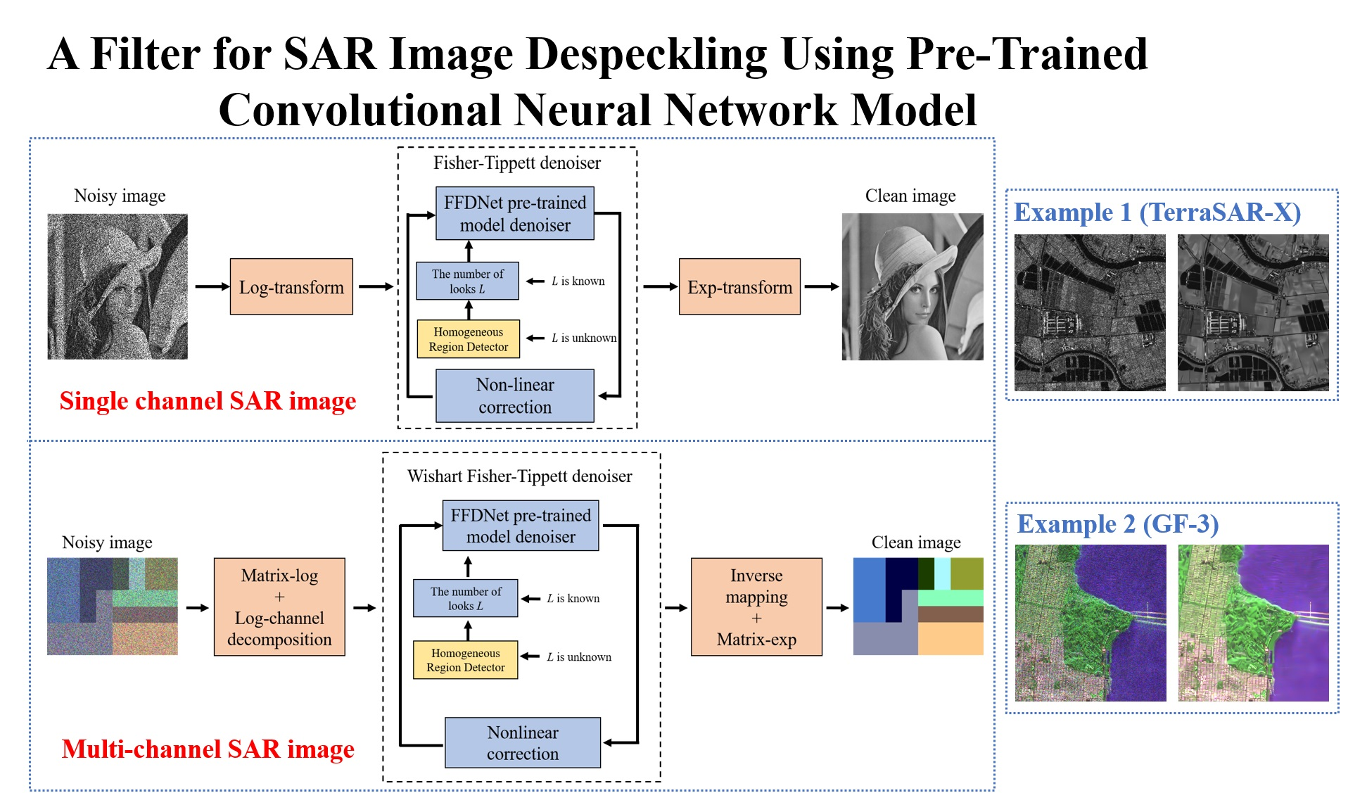
To avoid the preparation of huge SAR dataset, well-designed network or loss function, and complicated training, the work in [36] directly embedded the pre-trained CNN model [30], which was trained on abundant nature gray images with AWGN, with the MuLoG framework [29] for SAR despeckling, and it achieved the satisfying performance. However, the problem in [36] is that 14 pre-trained models for specific preset noise levels were utilized. When the images have real noise levels that are not the preset ones, they are more likely to be over-smoothed (if the preset noise level is bigger than the real one) or under-smoothed (if the preset noise level is smaller than the real one). To solve this problem, we adopt a new pre-trained CNN model, FFDNet [31]. In FFDNet, a two-dimensional noise level map is taken as an input to the model training, thus the model parameters are invariant to the noise level. In this way, only a single pre-trained model is needed to denoise images with different noise levels in preset range, i.e. [0, 75], and better denoising results will be obtained. Moreover, when the number of looks L of SAR images is not clear, we employ the method in [37] to find the homogeneous region in the SAR images without any interaction to estimate the noise level, i.e., the number of looks L, as the input to the network. Combining the homogeneous region detector with FFDNet, we are able to denoise the single channel or multi-channel SAR images in an end-to-end way in the framework of MuLoG [29].

The contributions of this paper are:

• Following the work of Yang [36], we adopt a new pre-trained CNN model, FFDNet. Taking the noise level as input to network training, FFDNet can obtain a more precise despeckling no matter what the noise level is. Combining MuLoG with pre-trained FFDNet model, this despeckling filter can not only handle single channel but also multi-channel SAR images.
• We propose to use the homogeneous region detector to calculate the number of looks, L, which makes the despeckling framework work in an end-to-end way.
• Experiments on simulated and real (Pol)SAR images demonstrate the superior despeckling ability of our proposed method.

The remainder of this paper is organized as follows. Section 2 and Section 3 introduce the proposed despeckling methods for SAR or PolSAR image, respectively. Next, experimental results are given in Section 4. Finally, the discussion and the conclusions are presented in Section 5 and Section 6, respectively.

2. Despeckling Filter for SAR Images

2.1. A Gaussian Denoiser: FFDNet

For additive white Gaussian noise (AWGN), image denoising methods can be divided into two major categories: model based methods and discriminative learning based ones. Although model based methods, such as BM3D [21], are designed to model image priors and always have state-of-the-art denoising performances with various noise level, they are always time consuming and need to be carefully designed. To overcome the limitations of model based methods, several discriminative learning based methods are proposed, which learn the underlying images prior and fast inference with training. Among them, convolutional neural networks (CNN) based denoisers [30,31] have achieved very competitive denoising performance.

FFDNet [31] is a fast and flexible CNN based Gaussian denoiser which learns the “clean” images from noisy ones. Figure 1 illustrates the architecture of FFDNet. This network is modified from the famous VGG network [38], which consists of a series of $3\times 3$ convolutional layers without pooling. Each layer is composed of a specific combination: Convolution (Conv), Rectified Linear Units (ReLU) [39], and Batch Normalization (BN) [40]. Specifically, “Conv + ReLU” is adopted for the first layer, “Conv + BN + ReLU” for middle layers, and “Conv” for the last convolution layer. Zero-padding is employed to keep the size of feature maps unchanged after each convolution. Two highlights of FFDNet are:

• Downsampling and Upsampling. As the efficiency is a crucial issue for CNN-based denoising methods, a reversible downsampling layer is added to reshape the input image into a set of sub-images which can also effectively expand the receptive filed. A upsampling operation is applied in the last layer. In [31], the downsampling factor is set to 2.
• Noise Level Map, M. Being different from other CNN-based denoisers, FFDNet takes a tunable noise map M as input to network to handle different noise levels with a single model. The noise map M can make a trade-off between noise reduction and detail preservation.

The denoising problem in FFDNet can be written as [31]:

$$\widehat{x}=\mathcal{F}(y,M;\Theta ),$$

(1)

where $\mathcal{F}$ is a mapping function between the noisy observation y and $\widehat{x}$. $\widehat{x}$ is the estimation of the desired “clean” image x, and $\Theta$ is the underlying model parameters. Before feeding data into network, the input image of size $W\times H\times C$ is downsampled into four sub-images with size of $\frac{W}{2}\times \frac{H}{2}\times 4C$ (the downsampling factor is 2 in both hight and width), where C is the number of channels. Then, noise level map M is concatenated to form a tensor of size $\frac{W}{2}\times \frac{H}{2}\times (4C+1)$ as the input to CNN. In the training step, about 5544 natural gray images are used, and the patch size is set as $70\times 70$ pixels. In each epoch, $N=128\times 8000$ patches are added AWGN of a random noise level $\sigma \in [0,75]$ to get noisy patches [31],

$$y=x+\frac{\sigma }{255}N(0,1).$$

(2)

It is worth noting that the elements in M are all $\sigma$. To train the model, the loss function is defined as the mean square error (MSE) between $\widehat{x}$ and ground truth x [31]:

$$\mathcal{L}(\Theta )=\frac{1}{2N}\sum _{i=1}^N{∥\mathcal{F}\left(y_i,M_i;\Theta \right)-x_i∥}^2.$$

(3)

where ${\left\{\left(y_i,{\mathit{M}}_i;x_i\right)\right\}}_{i=1}^N$ represents input–output pairs. After 80 epochs of training, we can get a single pre-trained FFDNet for gray images with different noise level AWGN.

2.2. Homogeneous Region Detector

As mentioned above, the noise level is one of the inputs to the network, which means we need to know the noise level $\sigma$ of the noisy image. For SAR or PolSAR images, the noise level is always related to the number of looks L. To obtain the L, one common way is to find several visual homogeneous regions, and then calculate the L using their mean and standard deviation. When the number of looks is not known, this procedure makes denoising to be a two stage problem: estimate L and filtering. To make denoising as an end-to-end problem, we utilize the idea in [37] to find homogeneous areas in SAR images automatically without any prior information.

In the homogenous areas, the signal fluctuations can be assumed to be negligible compared to the noise fluctuations, thus the noise statistics can be estimated from these areas. In [37], the image is first divided into small square regions, and then a non-parametric homogeneous region detector is designed to answer the following statistical hypothesis test:

$$\begin{array}{cc}{H}_0:B\mathrm{is}\mathrm{homogeneous}\hfill & (\mathrm{null}\mathrm{hypothesis})\hfill \\ H_1:B\mathrm{is}\mathrm{inhomogeneous}\hfill & (\mathrm{alternative}\mathrm{hypothesis}).\hfill \end{array}$$

(4)

where B is the fixed size square block. Based on the proposition that, if two random disjoint sequences P and Q of a block are correlated, i.e., $\mathrm{Corr}(P,Q)\ne 0$, then the block is inhomogeneous. And a score $s:{\mathbb{R}}^n\times {\mathbb{R}}^n\to \mathbb{R}$ should be designed to answer above hypothesis problem. The score s should promise that for any $P_{\mathrm{FA}}\in [0,1]$, there exists a threshold $\alpha >0$ satisfying [37]:

$$\underset{n\to \infty }{\lim }\mathbb{P}\left(\underset{\mathrm{false}\mathrm{alarms}}{\underbrace{\left|s\right(P,Q\left)\right|\ge \alpha }}|H_0\right)=P_{\mathrm{FA}},$$

(5)

$$\underset{n\to \infty }{\lim }\mathbb{P}\left(\underset{\mathrm{miss}\mathrm{detections}}{\underbrace{\left|s\right(P,Q\left)\right|<\alpha }}|H_1\right)=0.$$

(6)

where n is the number of elements in P or Q. To make the test of homogeneity independent of the noise distribution, the rank of the values is considered. The block is homogeneous if the ranking of the pixel values is uniformly distributed. Thus, the Kendall’s $\tau$ coefficient [41,42] is used to assessed such correlation between random sequences in the block, which depends only on the relative order of the values of P and Q [37]:

$$\tau (P,Q)=\frac{1}{n(n-1)}\sum _{1\le i,j\le n}\mathrm{sign}\left(P_i-P_j\right)\mathrm{sign}\left(Q_i-Q_j\right),$$

(7)

where $P\in {\mathbb{R}}^n$, $Q\in {\mathbb{R}}^n$, and $\tau :{\mathbb{R}}^n\times {\mathbb{R}}^n\to [-1,1]$. $P_i$ is the ith elements of P.

Once the homogenous regions are found, the value of L can be easily calculated. One of the advantages of this detector is that it has a non-detection rate independent of the unknown distribution of the noise. Thus, it can be employed to SAR images even the speckle is always multiplicative.

2.3. Homo-FFDNet Filter for SAR Images

According to Goodman’s model [2], the intensity (the square of modulus) of SAR images follows a gamma distribution $\mathcal{G}(R;L)$ whose probability density is:

$$p_I\left(I\right|R)=\frac{L^L{I}^{L-1}}{\Gamma \left(L\right)R^L}\exp \left(-L\frac{I}{R}\right),$$

(8)

where $I\in {\mathbb{R}}_{+}$ is the observed intensity and $R\in {\mathbb{R}}_{+}$ is the underlying reflectivity. The number of looks L satisfies $L>0$, and the $\Gamma$ means the gamma function. The intensity of SAR is disturbed by signal dependent multiplicative fluctuations S which follows a standard gamma distribution ($S\sim \mathcal{G}(1;L)$):

$$I=R\times S.$$

(9)

There are many ways to estimate the underlying reflectivity R, among which homomorphic approach is a simple and straight one. The logarithm $y=\log I\in \mathbb{R}$ is used to transfer the multiplicative fluctuations S to the additive ones. Then, a Gaussian denoiser for AWGN comes into play. After log-transforming, $y=\log I$ follows the Fisher–Tippett distribution, denoted as $\mathcal{F}\mathcal{T}(x;L)$ [43]:

$$p_y\left(y\right|x)=\frac{L^L}{\Gamma \left(L\right)}{e}^{L(y-x)}\exp \left(-L{e}^{y-x}\right),$$

(10)

where $x=\log R\in \mathbb{R}$. It should be pointed out that the theoretical variance of y is $\Psi (1,L)$ where $\Psi (·,L)$ is the polygamma function of order L. If we cannot know the value of L in advance, L can be calculated with the help of homogeneous region detector. A classical approach to estimate x is to approximate the Fisher–Tippett distribution by a non-centered Gaussian distribution [29]:

$$\widehat{x}=f_{\Psi (1,L)}\left(y\right)+\underset{\mathrm{debiasing}}{\underbrace{(\log L-\Psi (L\left)\right)}},$$

(11)

where $f_{{\sigma }^2}:{\mathbb{R}}^n\to {\mathbb{R}}^n$ is a denoiser for zero-mean additive white Gaussian noise $\mathcal{N}\left(0;{\sigma }^2\right)$, and $\Psi (·)$ is the digamma function. Finally, the estimated $\widehat{R}$ can be obtained by an exponential operation $\widehat{R}=\exp \left(\widehat{x}\right)$. It is worth noting that a debiasing step is necessary as we assumed a non-zero mean noise to be a zero-mean one. Here, we choose the pre-trained FFDNet model as the Gaussian denoiser f in Equation (11). Being similar to the preprocessing in the test step in FFDNet, normalization should be done to the SAR intensity as the input to the network:

$$y_{input}=\left(y-y_{\min }\right)/\left(y_{\max }-y_{\min }\right),$$

(12)

where $y_{\min }$ is the $0.3\%$ quantile of y and $y_{\max }$ is the $99.7\%$ quantile of y. Here, $0.3\%$ and $99.7\%$ are empirical values according to the 3$\sigma$ criterion. This is to eliminate the effects of heavy left tail in Fisher–Tippet distribution as well as removing outliers. The variance of the intensity which is used to form the noise level map M should also be normalized:

$$\mathrm{Var}\left(y_{input}\right)=\Psi (1,L)/{\left(y_{\max }-y_{\min }\right)}^2.$$

(13)

Finally, the normalized intensity and variance are taken as inputs into pre-trained FFDNet to get the “clean” image $\widehat{x}$. After debiasing and exp-transformation, the filtered SAR image can be obtained. The framework of the homomorphic approach, named Homo-FFDNet, is displayed in Figure 2.

2.4. MuLoG-FFDNet Filter for SAR Images

Rather than estimating the log-transformed reflectivity x by a Gaussian distribution such as homomorphic approach, the MuLoG algorithm [29] adopts variational approach directly which considers the Fisher–Tippett distribution in log domain, leading to a MAP optimization problem [44,45]:

$$\widehat{x}\in \underset{\widehat{x}\in {\mathbb{R}}^n}{\mathrm{argmin}}\left(-\log p_y\left(y\right|x)+\mathcal{R}\left(x\right)\right)$$

(14)

$$-\log p_y\left(y\right|x)=L\sum _{i=1}^n{x}_i+e^{y_i-x_i}+\mathrm{Cst}.$$

(15)

where $\mathcal{R}\left(x\right)=-\log p_x\left(x\right)$ is a prior term enforcing some regularity on the solution, n is the number of pixels in image, and $\mathrm{Cst}.$ is a constant. The problem in Equation (14) is a generic unconstrained optimization, and it can be solved by using the plug-and-play Alternating Direction Method of Multipliers (ADMM) algorithm [46], which repeats the updates:

$$x^{(k+1)}=\underset{x\in {\mathbb{R}}^n}{\mathrm{argmin}}\left(-\log p_y\left(y\right|x)+\frac{\rho }{2}{∥x-\left(v^{\left(k\right)}-u^{\left(k\right)}\right)∥}^2\right)$$

(16)

$$v^{(k+1)}=f_{{\sigma }_k}\left(x^{(k+1)}+u^{\left(k\right)}\right)$$

(17)

$$u^{(k+1)}=u^{\left(k\right)}+\left(x^{(k+1)}-v^{(k+1)}\right)$$

(18)

where k means the $k\mathrm{th}$ $(k=1,2,\dots ,K)$ iteration, and K is set to 6 in all the experiments presented in this paper. $f_{{\sigma }_k}$ is a Gaussian filter with the noise variance ${\sigma }_k$. In [29], the ${\sigma }_k$ is chosen as $\sqrt{1/\rho }$, and the internal parameter $\rho =(1+2/L)/\Psi (1,L)$. The homogeneous region detector can be used here to calculate L. The minimization of x in Equation (16) amounts to solving n separable convex problems, which can be solved efficiently with 10 iterations of Newton’s method [46]. In MuLoG framework, Equation (17) is done by a Gaussian filter, and, in our proposed method, $f_{{\sigma }_k}$ is the pre-trained FFDNet model. Equations (17) and (18) work for non-linear correction. After six iterations, an exp-transformation is operated on $\widehat{x}$ to get the final estimate $\widehat{R}$. The framework of MuLoG-FFDNet filter for single channel SAR images is displayed in Figure 3.

3. Despeckling Filter for PolSAR Images

PolSAR images carry more information than single channel SAR images. For the monostatic fully PolSAR images, the lexicographic scatter vector $\mathbf{k}$ is defined as:

$${\mathbf{k}}_{3L}={\left[S_{hh},\sqrt{2}{S}_{hv},S_{vv}\right]}^T,$$

(19)

where h and v are the polarization states and ${}^T$ is transposition operation. Suppose there are L independent random scattering vector samples following the D-dimensional complex circular Gaussian distribution, $\left\{{\mathbf{k}}_1,\cdots ,{\mathbf{k}}_L\right\}$, satisfying $L>D$ ($D=3$). Then, the covariance matrix $\mathit{C}$ can be defined as the mean of $\mathbf{k}$’s inner product:

$$\mathit{C}=\frac{1}{L}\sum _{i=1}^L{\mathbf{k}}_i{\mathbf{k}}_i^H,$$

(20)

where ${}^H$ means complex conjugate transpose. According to Goodman’s model [2], the covariance matrix follows the complex Wishart distribution $\mathcal{W}(\mathsf{\Sigma };L)$:

$$\mathit{C}={\mathsf{\Sigma }}^{1/2}\mathit{S}{\mathsf{\Sigma }}^{1/2},$$

(21)

$$p_{\mathit{C}}\left(\mathit{C}\right|\mathsf{\Sigma })=\frac{L^{LD}{\left|\mathit{C}\right|}^{L-D}}{{\Gamma }_D\left(L\right){\left|\mathsf{\Sigma }\right|}^L}\exp \left(-L\mathrm{tr}\left({\mathsf{\Sigma }}^{-1}\mathit{C}\right)\right),$$

(22)

where $\mathsf{\Sigma }$ is the underlying covariance matrix and $\mathit{S}$ is the speckle. Both $\mathit{C}$ and $\mathsf{\Sigma }$ belong to the open cone of complex Hermitian positive definite matrices. To use the MuLoG algorithm [29], the covariance matrix $\mathit{C}$ should be transformed into log domain. Here, a matrix logarithm is used to convert the multiplicative speckle into additive ones, $\mathsf{\Sigma }\mapsto \tilde{\mathsf{\Sigma }}=\log \mathsf{\Sigma }$, and the matrix exponential is defined similarly, $\tilde{\mathsf{\Sigma }}\mapsto \mathsf{\Sigma }=e^{\tilde{\mathsf{\Sigma }}}$. The log-transformed matrix $\tilde{\mathit{C}}$ follows the Wishart–Fisher–Tippett distribution [29]:

$$\mathrm{tr}\tilde{\mathit{C}}=\mathrm{tr}\tilde{\mathsf{\Sigma }}+\mathrm{tr}\tilde{\mathit{S}}$$

(23)

$$p_{\tilde{\mathit{C}}}(\tilde{\mathit{C}}|\tilde{\mathsf{\Sigma }})=\frac{L^{LD}f\left(\tilde{\mathit{C}}\right)}{{\Gamma }_D\left(L\right)}{e}^{L\mathrm{tr}(\tilde{\mathit{C}}-\tilde{\mathsf{\Sigma }})}\exp \left(-L\mathrm{tr}\left(e^{\tilde{\mathit{C}}}{e}^{-\tilde{\mathsf{\Sigma }}}\right)\right).$$

(24)

After matrix log transformation, a re-parameterization method [29] which represents the log-transformed covariance matrix $\tilde{\mathit{C}}$ as a real vector $\mathit{y}$ is proposed, denoted as $\tilde{\mathit{C}}=\Omega \left(\mathit{y}\right)$. Here, the noise in each of $\mathit{y}$’s channels $y^i,i=1,\dots ,D^2$ (D = 3) is assumed to be signal independent, and the noise variance is about the same for all channels. As for PolSAR, the MAP optimization problem in Equations (14) and (15) is redefined as:

$$\widehat{\mathit{x}}\in \underset{\mathit{x}}{\mathrm{argmin}}\left(-\log p_{\mathit{y}}\left(\mathit{y}\right|\mathit{x})+\sum _{i=1}^{D^2}\mathcal{R}\left(x^i\right)\right)$$

(25)

$$-\log p_{\mathit{y}}\left(\mathit{y}\right|\mathit{x})=L\sum _{k=1}^n\mathrm{tr}\left(\Omega \left({\mathit{x}}_{\mathit{k}}\right)+e^{\Omega \left({\mathit{y}}_{\mathit{k}}\right)}{e}^{-\Omega \left({\mathit{x}}_{\mathit{k}}\right)}\right)+\mathrm{Cst}.$$

(26)

where $\tilde{\mathsf{\Sigma }}=\Omega \left(\mathit{x}\right)$, n is the number of pixel and ${\mathit{x}}_{\mathit{k}}$ means the kth pixel. When $D=1$, this MAP problem is exactly the same as single channel case. Finally, the estimated $\widehat{\mathsf{\Sigma }}$ can be obtained by $\widehat{\mathsf{\Sigma }}=\exp \Omega \left(\widehat{\mathit{x}}\right)$. To solve the MAP optimization problem, the ADMM algorithm is used. We also use the pre-trained FFDNet model as Gaussian denoiser. However, as suggested by Deledalle et al. [29], the value of ${\sigma }_k$ is 1 in the initial iteration and $1+2/L$ in the following iterations. Here, the number of iterations is also set as 6. Figure 4 gives the framework of despeckling PolSAR images with pre-trained model embedded with MuLoG.

4. Experimental Results

4.1. Experiments for SAR Images

Numerical experiments were conducted using by pre-trained FFDNet models for SAR images. The proposed methods Homo-FFDNet and MuLoG-FFDNet were compared to the homomorphic method with block-matching and 3D filtering (Homo-BM3D) [29], MuLoG method with BM3D denoiser (MuLoG-BM3D) [29], homomorphic method with pre-trained DnCNN model (Homo-DnCNN) [36], and MuLoG method with pre-trained DnCNN model (MuLoG-DNCNN) [36].

To simulate SAR images, different levels of speckle ($L=1,2,4,5,10,15,20$) were added to the famous Lena image with size of $512\times 512$ pixels. Only the simulated images of $L=1,4$ are shown in Figure 5. To quantitatively evaluate the performance of all filters for simulated SAR images, peak signal noise ratio (PSNR), up to most recent indexes, was first chosen to measure the amplitude reconstruction. Structural preservation index measurement (SSIM) [47] can also provide meaningful information about the closeness of two images from the point of their structural information. Equivalent number of looks (ENL) was also used to measure the degree of speckle suppression when homogeneous areas are provided. For PSNR and ENL, the higher value is better, but, for SSIM, the value closest to 1 is better. We also used the homogeneity index $\delta h$ of $\mathcal{M}$-index proposed in [48] to measure the detail preservation. For $\delta h$, a smaller value means better detail preservation.

Figure 6 and Figure 7 show the filtered results of simulated SAR images with L = 1 and L = 4, respectively. Considering high level of noise with L = 1, as shown in Figure 6, the homomorphic approach using pre-trained model (DnCNN or FFDNet) tends to leave residual dark strains and over-smooth bright targets, to some degree, revealing its lack of robustness against the heavy left tail of the Fisher–Tippet distribution. However, the Homo-FFDNet performs better than Homo-DnCNN, as fewer residual dark strains are left. Comparing with homomorphic approach, the MuLoG based methods seem to show a good speckle suppression and the ability to remove artifacts, among which the MuLoG-FFDNet is the best. The filter result of MuLoG-BM3D has a “piece by piece” appearance, while MuLoG-DnCNN and MuLoG-FFDNet look much smoother. It is worth noting that MuLoG-FFDNet has good smoothing and better detail preservation than MuLoG-DnCNN. For example, MuLoG-DnCNN still has a little residual dark strain on Lena’s shoulder while MuLoG-FFDNet does not. Looking at the brim of Lena’s hat, MuLoG-FFDNet obviously retains more image details, as shown by the zoomed in image. The pre-trained FFDNet model introduces a noise level map M, which plays the role of controlling the trade-off between noise reduction and detail preservation. In addition, being trained with abundant clean–noisy image pairs, FFDNet has the strength to preserve details well. The quantitative results are provided in

Table 1. The quantitative comparison of different methods for simulated SAR image with $L=1$.

Method	PSNR	SSIM	ENL(A1)	ENL(A2)	$\mathit{\delta }\mathit{h}$
Noisy	10.65	0.3316	1.11	0.96	-
Homo + BM3D	25.19	0.7957	97.75	143.47	9.017
MuLoG + BM3D	26.65	0.8394	120.21	213.53	11.71
Homo + DnCNN	25.55	0.8060	132.27	153.99	6.457
MuLoG + DnCNN	26.80	0.8526	255.06	216.64	16.30
Homo + FFDNet	26.12	0.8314	198.74	204.21	4.511
MuLoG + FFDNet	27.09	0.8605	342.09	243.50	13.90

, and the ENL was computed using homogeneous areas $A1$ and $A2$ displayed in Figure 5a. When considering low level of noise with L = 4, MuLoG based methods are still more promising in the vision than the Homo based methods in Figure 7. The quantitative results are provided in

Table 2. The quantitative comparison of different methods for simulated SAR image with $L=4$.

Method	PSNR	SSIM	ENL(A1)	ENL(A2)	$\mathit{\delta }\mathit{h}$
Noisy	16.33	0.5393	3.82	3.73	-
Homo + BM3D	29.98	0.9088	155.32	138.37	19.08
MuLoG + BM3D	29.98	0.9138	115.53	154.15	18.40
Homo + DnCNN	30.16	0.9182	158.55	141.42	22.61
MuLoG + DnCNN	30.30	0.9198	159.68	167.54	11.93
Homo + FFDNet	30.47	0.9272	180.58	147.02	15.34
MuLoG + FFDNet	30.60	0.9272	184.93	176.55	9.756

.

Considering the homogeneity index, $\delta h$, we can find that, when the noise level of image is high (L = 1), Homo based methods seem to have a better detail preservation than MuLoG based methods. MuLoG based methods tend to have an over-smoothing. However, when the noise level of image is low (L = 4), MuLoG based methods perform better. Figure 8 gives the change trends of PSNR and SSIM with different L. We can see that MuLoG-FFDNet has robust performance.

Two TerraSAR-X images in Guangzhou with size of $500\times 500$ pixels were also tested, as shown in Figure 9. Being different from simulated SAR image, real SAR image does not have a clean reference, thus ENL and visual inspection are the best ways to do the qualitative and quantitative analysis. To verify the ability of edge preservation of the proposed filter, the ratio of average (EPD-ROA) [49] was also computed along the horizontal direction (HD) and vertical direction (VD). $\delta h$ was used to evaluate the detail preservation. The denoising results for two real SAR images are given in Figure 10 and Figure 11, respectively. The values of ENL (computed in areas $B\left(C\right)1$ and $B\left(C\right)2$) and EPD-ROA (computed in areas $B\left(C\right)3$ and $B\left(C\right)4$) are also provided in

Table 3. The quantitative comparison of different methods for real SAR image: Data 1.

Method	ENL(B1)	ENL(B2)	ERI-ROA(B3)		ERI-ROA(B3)		$\mathit{\delta }\mathit{h}$
			HD	VD	HD	VD
Noisy	1.083	0.9028	-	-	-	-	-
Homo + BM3D	42.68	35.72	0.2606	0.3311	0.4076	0.3771	1.375
MuLoG + BM3D	43.12	36.74	0.3060	0.3563	0.3788	0.3820	3.032
Homo + DnCNN	68.52	37.28	0.3037	0.3484	0.4029	0.3955	8.940
MuLoG + DnCNN	80.71	55.35	0.3148	0.3557	0.4170	0.3987	5.489
Homo + FFDNet	86.59	54.39	0.3449	0.3866	0.3905	0.3944	0.1472
MuLoG + FFDNet	95.69	61.71	0.3479	0.3942	0.3960	0.3949	2.669

and

Table 4. The quantitative comparison of different methods for real SAR image: Data 2.

Method	ENL(C1)	ENL(C2)	ERI-ROA(C3)		ERI-ROA(C4)		$\mathit{\delta }\mathit{h}$
			HD	VD	HD	VD
Noisy	1.36	1.37	-	-	-	-	-
Homo + BM3D	80.67	57.67	0.3579	0.3621	0.3384	0.3762	1.965
MuLoG + BM3D	83.06	56.16	0.3572	0.3700	0.3487	0.3904	11.71
Homo + DnCNN	161.72	67.18	0.3707	0.3702	0.3622	0.4125	2.762
MuLoG + DnCNN	339.34	200.37	0.3784	0.3782	0.3494	0.4110	14.49
Homo + FFDNet	176.00	83.66	0.3729	0.3711	0.3503	0.3929	4.681
MuLoG + FFDNet	414.80	205.60	0.3868	0.3835	0.3588	0.3969	10.91

for comparison. Because the information about L is not very clear for these two SAR images, we used homogeneous region detector to calculate the value of L. For Data 1, the computed $L=$ 1.11, while, for Data 2, $L=1.46$.

4.2. Experiments for PolSAR Images

Our framework, which embeds MuLoG with pre-trained FFDNet can not only handle single channel SAR images, but also multi-channel SAR images. We chose refined Lee filter, IDAN, MuLoG-BM3D, and MuLoG-DnCNN for comparison purpose. For refined Lee Filter, the size of the filtering window was set to be $7\times 7$. The IDAN filter was tested by using a maximum adaptive neighborhood size of 15 pixels. For both simulated PolSAR images and real ones, ENL and ERI-ROA were still computed to evaluate the performance of these filters quantitatively.

We followed the method mentioned in [1] to generate simulated PolSAR images with $L=1$ and $L=4$ and size of $300\times 300$ pixels, as displayed in Figure 12. The visual filtered results and the nine components of $\mathit{x}$ (${\mathit{x}}^{\mathbf{1}}$, ${\mathit{x}}^{\mathbf{2}}$, …, ${\mathit{x}}^{\mathbf{9}}$) for the image of the covariance matrix $\mathit{C}$ are displayed in Figure 13 and Figure 14. When the noise level is high, e.g., L = 1, the MuLoG based methods have an obvious strength in smoothing than refined Lee filter and IDAN, whose filtering results retain many speckles. To be specific, the MuLoG-FFDNet is the best, while MuLoG-DnCNN is almost the same. However, looking carefully, some stains are still left in the result of MuLoG-DnCNN while the performance of MuLoG-FFDNet is good, no matter its ability to speckle suppression or detail preservation. The quantitative comparisons are also provided in

Table 5. The quantitative comparison of different methods for simulated PolSAR image with $L=1$.

Method	ENL(D1)	ENL(D2)	ERI-ROA(D3)		ERI-ROA(D3)
			HD	VD	HD	VD
Noisy	1.019	1.020	-	-	-	-
Refined Lee	26.47	27.83	0.5726	0.5425	0.4803	0.4855
IDAN	8.521	13.18	0.5626	0.5380	0.4901	0.4944
MuLoG + BM3D	113.40	206.82	0.5630	0.5380	0.4819	0.4825
MuLoG + DnCNN	394.61	854.78	0.5731	0.5393	0.4817	0.4823
MuLoG + FFDNet	592.73	1353.2	0.5767	0.5449	0.4919	0.4819

and

Table 6. The quantitative comparison of different methods for simulated PolSAR image with $L=4$.

Method	ENL(D1)	ENL(D2)	ERI-ROA(D3)		ERI-ROA(D4)
			HD	VD	HD	VD
Noisy	3.962	3.925	-	-	-	-
Refined Lee	93.76	113.14	0.8333	0.8488	0.8813	0.8707
IDAN	64.24	62.99	0.8303	0.8503	0.8828	0.8694
MuLoG + BM3D	213.37	180.72	0.8313	0.8488	0.8829	0.8698
MuLoG + DnCNN	750.81	863.36	0.8324	0.8490	0.8818	0.8743
MuLoG + FFDNet	1860.6	1174.9	0.8340	0.8513	0.8823	0.8738

(ENL was computed in areas $D1$ and $D2$, ERI-ROA was computed in areas $D3$ and $D4$). Whether the noise level is high or low, the performance of the MuLoG-FFDNet is very robust.

We next used two real PolSAR images: one is a fully polarimetric SAR image obtained by CETC-38th airborne SAR system in Lingshui city of China with the number of looks $L=1$ and size of $500\times 500$ pixels and the other is a fully polarimetric GF-3 image over San Francisco with L=1, and size of $500\times 500$ pixels. The visual filtered results are given in Figure 15 and Figure 16. The quantitative results are provided in

Table 7. The quantitative comparison of different methods for CETC-38th airborne SAR.

Method	ENL(E1)	ENL(E2)	ERI-ROA(E3)		ERI-ROA(E4)
			HD	VD	HD	VD
Noisy	0.9790	0.8894	-	-	-	-
Refined Lee	23.80	21.01	0.4681	0.4003	0.3402	0.3970
IDAN	13.11	11.47	0.4478	0.3323	0.2479	0.3101
MuLoG + BM3D	165.09	58.84	0.4391	0.4917	0.2752	0.5059
MuLoG + DnCNN	284.50	37.46	0.4460	0.4793	0.3268	0.4947
MuLoG + FFDNet	385.86	92.48	0.4566	0.4106	0.3802	0.4234

and

Table 8. The quantitative comparison of different methods for GF-3.

Method	ENL(F1)	ENL(F2)	ERI-ROA(F3)		ERI-ROA(F4)
			HD	VD	HD	VD
Noisy	0.9333	0.9178	-	-	-	-
Refined Lee	10.68	11.34	0.3039	0.4704	0.3114	0.4547
IDAN	4.82	4.56	0.2735	0.4323	0.2821	0.4355
MuLoG + BM3D	89.44	76.20	0.2891	0.4028	0.2984	0.3896
MuLoG + DnCNN	124.40	158.20	0.3039	0.4268	0.3117	0.4046
MuLoG + FFDNet	140.47	159.18	0.3155	0.4361	0.3188	0.4102

(ENL was computed in areas $E\left(F\right)1$ and $E\left(F\right)2$, ERI-ROA was computed in areas $E\left(F\right)3$ and $E\left(F\right)4$).

PolSAR image despeckling is an important preprocessing step before extracting land-object information. A state-of-the-art filter should not only effectively suppress the speckle and preserve the edge, but also enhance the differences between various classes and preserve the polarimetric scattering mechanism. Thus, the scatter grams of the Cloude polarimetric decomposition parameters (entropy H, anisotropy A, and alpha angle $\alpha$) [50] for three areas (marked with white squares in Figure 8 and Figure 15) with different land-object types are provided in Figure 17 and Figure 18 for two PolSAR data, respectively. The entropy H describes the degree of statistical disorder of each distinct scatter type within the ensemble; the anisotropy A measures the relative importance of the second and the third eigenvalues of the eigen decomposition; and the angle $\alpha$ is related to the underlying average physical scattering mechanism. First, various kinds of land-objects are much more separable after filtering due to the suppression of the speckle. Then, compared with refined Lee and IDAN, MuLoG based methods can not only preserve the polarimetric scattering mechanism well but also make the various land-object more separable.

4.3. Experiments for Homogeneous Region Detector

We used simulated single channel SAR images to validate the effectiveness of homogeneous region detector. Several simulated images with different numbers of looks L, ($L=1,2,4,5,10,15,20$) were generated, and the homogeneous region detector was used to find the homogeneous region of each SAR images. Once the regions were found, they were used to calculate L. Figure 19 shows the results, where the red “∘” is the ground truth of L, the green “×” means L was computed by homogeneous region detector (HRD), and the blue “⋆” means homogeneous regions (HR) was found by manual operation. In Figure 19, we can see the values of L computed by homogeneous region detector are the closest to the ground truth.

Table 9. The quantitative comparison of different methods for simulated SAR image with $L=1$.

Method	PSNR	SSIM	ENL(A1)	ENL(A2)
Homo + FFDNet+gt	26.12	0.8314	198.74	204.21
Homo + FFDNet+HRD	26.16	0.8326	199.77	204.79
Homo + FFDNet+HR	26.08	0.8301	197.40	203.61
MuLoG + FFDNet+gt	27.09	0.8605	342.09	243.50
MuLoG + FFDNet+HRD	27.11	0.8611	346.37	244.00
MuLoG + FFDNet+HRD	27.08	0.8602	340.37	243.34

gives the quantitative comparison on simulated filtered SAR image.

4.4. Computation Time Analysis

We tested the computation time using a single channel SAR image with size of $512\times 512$ pixels. The computation time of different methods are provided in

Table 10. The computation time of different methods.

Method	Homo + BM3D	Homo + DnCNN	Homo + FFDNet	MuLoG + BM3D	MuLoG + DnCNN	MuLoG + FFDNet
Time (second)	3.02 s	0.89 s	0.78 s	17.59 s	5.25 s	4.21 s

. The computer that we used is with a Inter(R) Core(TM) i7-8700 CPU @3.20 GHz, 16 GB RAM and a Nvidia GeForce GTX 1050 Ti GPU. The Homo+BM3D and MuLoG+BM3D were performed in Matlab (R2017a) environment with the code provided by the author of MuLoG [29]. Homo+DnCNN, Homo+FFDNet, MuLoG+DnCNN, and MuLoG+FFDNet were performed in Python 3.6 and pytorch with GPU. The codes of these four methods were modified based on the source codes provided by the authors of DnCNN [30] and FFDNet [31], respectively.

Table 10 shows that the MuLoG based methods cost more time than the Homo based methods, as the formers involve iterations. The FFDNet based methods are a litter faster than the DnCNN based methods, because the downsampling operation in FFDNet accelerates the testing time.

5. Discussion

Speckle reduction is a key issue for SAR images, as it affects the accuracy and effectiveness of SAR images interpretation. In this paper, we propose to use the pre-trained FFDNet model with MuLoG framework to handle single channel or multi-channel SAR images. Our objective is to design a filter which can efficiently eliminate the speckle while having a good preservation of edge and details. With the help of noise level map, M, FFDNet based methods can solve the limitation in the methods proposed in [36], where over-smoothing or under-smoothing occurs. In addition, the homogeneous region detector helps make the proposed methods an end-to-end process. From the experimental results for both single channel SAR images and multi-channel SAR images, we can observe that, in terms of suppressing the speckle, the MuLoG based methods have superiority compared with Homo based methods. Among MuLoG based methods, MuLoG-FFDNet performs more robustly than MuLoG-DnCNN. The MuLoG-DnCNN may leave some spots on the images sometimes, while MuLoG-FFDNet always has an effective speckle reduction at various noise levels. As for detail preservation, MuLoG based methods tend to make some details over-smoothed, but they can remove the artifacts created by Homo based methods. Observing the zoom in parts in the filtered results, MuLoG-FFDNet has a better detail preservation than MuLoG-DnCNN. MuLoG based methods also make different land objects more separable while retaining the polarimetric scattering mechanisms well. When the value of L is unknown, the homogeneous region detector, which computes the number of looks L automatically, also has shown a satisfactory performance at various noise levels.

Using the pre-trained CNN model directly prevents us from preparing dataset, well designed network and tedious training to obtain state-of-the-art results. Moreover, as the lack of PolSAR data, no CNN-based methods have been proposed to despeckle PolSAR images. Maybe, a pre-trained filter on SAR images can be used to solve this problem embedded with MuLoG framework.

However, looking carefully at the filtered results of MuLoG-FFDNet, we can see the halo artifacts exist around the edges. Recently, a very simple but efficient idea to improve filter’s edge preservation capacity, called Side Window [51] has been proposed. Side Window changes the traditional center-based window into a side-based window, and can effectively restrain halo around edges. Although, the MuLoG framework is a non-patch based method, but the idea of Side Window can be used in the CNN network to train a filter with superior edge and detail preservation capacity in the future.

6. Conclusions

While most deep learning methods need many data or a well designed model, this paper proposes a simple yet efficient method which uses the pre-trained CNN model for SAR and PolSAR images despeckling embedded with MuLoG framework and a homogenous region detector. This pre-trained FFDNet model allows the proposed filter to work very robustly at various noise levels for single channel and multi-channel SAR images. Our work confirms that any superior Gaussian filter can be plugged into MuLoG framework to obtain the promising results in SAR images.

References

1. Lee, J.S.; Pottier, E. Polarimetric Radar Imaging: From Basics to Application; CRC Press: Boca Raton, FL, USA, 2009. [Google Scholar]
2. Goodman, J. Some fundamental properties of speckle. J. Opt. Soc. Am. 1976, 66, 1145–1150. [Google Scholar] [CrossRef]
3. Argenti, F.; Lapini, A.; Bianchi, T.; Alparone, L. A tutorial on speckle reduction in synthetic aperture radar images. IEEE Geosci. Remote Sens. Mag. 2003, 1, 6–35. [Google Scholar] [CrossRef]
4. Deledalle, C.A.; Denis, L.; Poggi, G.; Tupin, F.; Verdoliva, L. Exploiting patch similarity for sar image processing: the nonlocal paradigm. IEEE Signal Process. Mag. 2014, 31, 69–78. [Google Scholar] [CrossRef]
5. Lee, J.S. Digital image enhancement and noise filtering by use of local statistics. IEEE Trans. Pattern Anal. Mach. Intell. 1980, 2, 165–168. [Google Scholar] [CrossRef]
6. Lee, J.S. Refined filtering of image noise using local statistics. Comput. Gr. Image Process. 1981, 15, 380–389. [Google Scholar] [CrossRef]
7. Frost, V.S.; Stiles, K.S.; Shanmugan, K.S.; Holtzman, J.C. A model for radar images and its application to adaptive digital filtering of multiplicative noise. IEEE Trans. Pattern Anal. Mach. Intell. 1982, 4, 157–166. [Google Scholar] [CrossRef] [PubMed]
8. Kuan, D.T.; Sawchuk, A.A.; Strand, T.C.; Chavel, P. Adaptive noise smoothing filter for images with signal-dependent noise. IEEE Trans. Pattern Anal. Mach. Intell. 1985, 7, 165–177. [Google Scholar] [CrossRef] [PubMed]
9. Lopés, A.; Nezry, E.; Touzi, R.; Laur, H. Maximum a posteriori speckle filtering and first order texture models in SAR images. In Proceedings of the 10th Annual International Symposium on Geoscience and Remote Sensing (IGARSS), College Park, MD, USA, 20–24 May 1990; pp. 2409–2412. [Google Scholar]
10. Lattari, L.; Leno, B.G.; Asaro, F.; Rucci, A.; Prati, C.; Matteucci, M. Deep learning for SAR image despeckling. Remote Sens. 2019, 11, 1532. [Google Scholar] [CrossRef]
11. Sveinsson, J.R.; Benediktsson, J.A. Almost translation invariant wavelet transformations for speckle reduction of SAR images. IEEE Trans. Geosci. Remote Sens. 2003, 41, 2404–2408. [Google Scholar] [CrossRef]
12. Donoho, D.L. Deniosing by soft-thresholding. IEEE Trans. Inf. Theroy 1995, 41, 1953–1962. [Google Scholar]
13. Guo, H.; Odegard, J.E.; Lang, M. Wavelet based speckle reduction with application to SAR based ATD/R. In Proceedings of the International Conference on Image Processing(ICIP), Austin, TX, USA, 13–16 November 1994; pp. 75–79. [Google Scholar]
14. Xie, B.; Poerce, L.E.; Ulaby, F.T. SAR speckle reduction using wavelet denoising and Markov random field modeling. IEEE Trans. Geosci. Remote Sens. 2002, 40, 2196–2212. [Google Scholar] [CrossRef] [Green Version]
15. Achim, A.; Tsakalides, A.; Bezerianos, A. SAR image denoising via Bayesian wavelet shrinkage based on heavy-tailed modeling. IEEE Trans. Geosci. Remote Sens. 2003, 41, 1773–1784. [Google Scholar] [CrossRef]
16. Argenti, F.; Alparone, L. Speckle removal from SAR images in the undecimated wavelet domain. IEEE Trans. Geosci. Remote Sens. 2002, 40, 2363–2374. [Google Scholar] [CrossRef]
17. Li, H.C.; Hong, W.; Wu, Y.R.; Fan, P.Z. Bayesian wavelet shrinkage with heterogeneity-adaptive threshold for SAR image despeckling based on generalized gamma distribution. IEEE Trans. Geosci. Remote Sens. 2013, 51, 2388–2402. [Google Scholar] [CrossRef]
18. Zhang, W.G.; Zhang, Q.; Yang, C.S. Improved bilateral filtering for SAR image despeckling. Electron. Lett. 2011, 47, 286–288. [Google Scholar] [CrossRef]
19. Buades, A.; Coll, B.; Morel, J.M. A non-local algorithm for image denoising. In Proceedings of the Computer Vision and Pattern Recognition (ICCVPR), San Diego, CA, USA, 20–26 June 2005; pp. 60–65. [Google Scholar]
20. Deledalle, C.A.; Denis, L.; Tupin, F.; Reigber, A.; Jäger, M. NLSAR: A unified nonlocal framework for resolution-preserving (Pol)(In) SAR denoising. IEEE Trans. Geosci. Remote Sens. 2015, 53, 2021–2038. [Google Scholar] [CrossRef]
21. Kostadin, D.; Alessandro, F.; Vladimir, K. Image denoising by sparse 3-D transform-domain collaborative filtering. IEEE Trans. Image Process. 2007, 16, 2080–2095. [Google Scholar]
22. Parrilli, S.; Poderico, M.; Angelino, C.V.; Verdoliva, L. A Nonlocal SAR Image Denoising Algorithm Based on LLMMSE Wavelet Shrinkage. IEEE Trans. Geosci. Remote Sens. 2012, 50, 606–616. [Google Scholar] [CrossRef]
23. Rudin, L.; Lions, P.L.; Osher, S. Multiplicative Denoising and Deblurring: Theory and Algorithms. In Geometric Level Set Methods in Imaging, Vision, and Graphics; Springer: New York, NY, USA, 2003; pp. 103–119. [Google Scholar]
24. Durand, S.; Fadili, J.; Nikolova, M. Multiplicative noise removal using L1 fidelity on frame coefficients. J. Math. Imaging Vis. 2010, 36, 201–226. [Google Scholar] [CrossRef]
25. Tabti, S.; Deledalle, C.A.; Denis, L.; Tupin, F. Modeling the distribution of patches with shift-invariance: Application to SAR image restoration. In Proceedings of the IEEE International Conference on Image Processing (ICIP), Paris, France, 27–30 October 2014; pp. 96–100. [Google Scholar]
26. Liu, G.; Yang, W.; Xia, G.S. Structure preserveing SAR image despeckling via L0-minimazation. Prog. Electromagn. Res. 2013, 141, 347–367. [Google Scholar] [CrossRef]
27. González, A.A.; Martínez, C.L.; Salembier, P.; Deng, X.P. Bilateral distance based filtering for polarimatic SAR data. Remote Sens. 2013, 5, 5620–5641. [Google Scholar] [CrossRef]
28. Xing, X.L.; Chen, Q.H.; Yang, S.; Liu, X.G. Feature-based nonlocal polarimetric SAR filtering. Remote Sens. 2017, 9, 1043. [Google Scholar] [CrossRef]
29. Deledalle, C.A.; Denis, L.; Tabti, S.; Tupin, F. MuLoG, or How to apply Gaussian denoisers to multi-channel SAR speckle reduction? IEEE Trans. Image Process. 2017, 26, 4389–4403. [Google Scholar] [CrossRef] [PubMed]
30. Zhang, K.; Zuo, W.; Chen, Y.; Meng, D.; Zhang, L. Beyond a Gaussian denoiser: Residual learning of deep CNN for image denoising. IEEE Trans. Image Process. 2017, 26, 3142–3155. [Google Scholar] [CrossRef] [PubMed]
31. Zhang, K.; Zuo, W.; Zhang, L. FFDNet: Toward a fast and flexible solution for CNN-based image denoising. IEEE Trans. Image Process. 2017, 27, 4608–4622. [Google Scholar] [CrossRef]
32. Chierchia, G.; Cozzolino, D.; Poggi, G.; Verdoliva, L. SAR image despeckling through convolutional neural networks. In Proceedings of the IEEE International Geoscience and Remote Sensing Symposium (IGARSS), Fort Worth, TX, USA, 23–28 July 2017. [Google Scholar]
33. Wang, P.Y.; Zhang, H.; Patel, V.M. SAR image despecking using a convolutional neural network. IEEE Signal Process. Lett. 2017, 24, 1763–1767. [Google Scholar] [CrossRef]
34. Zhang, Q.; Yang, Z.; Yuan, Q.; Li, J.; Ma, X.; Shen, H.; Zhang, L. Learning a Dilated Residual Network for SAR Image Despeckling. Remote Sens. 2018, 10, 1–18. [Google Scholar] [CrossRef]
35. Yuan, Q.Q.; Zhang, Q.; Li, J.; Shen, H.F.; Zhang, L.P. Hyperspectral Image Denoising Employing a Spatial-Spectral Deep Residual Convolutional Neural Network. IEEE Trans. Geosci. Remote Sens. 2019, 57, 1205–1218. [Google Scholar] [CrossRef]
36. Yang, X.L.; Denis, L.; Tupin, F.; Yang, W. SAR image Depeckling using Pre-trained Convolutional Netural Network Models. In Proceedings of the Joint Urban Remote Sensing Event (JURSE), Vannes, France, 22–24 May 2019. [Google Scholar]
37. Sutour, C.; Deledalle, C.A.; Aujol, J.F. Estimation of the noise level function based on a nonparametric detection of homogeneous image regions. SIAM J. Imaging Sci. 2015, 8, 1–36. [Google Scholar] [CrossRef]
38. Simonyan, K.; Zisserman, A. Very Deep Convolutional Networks for Large-Scale Image Recognition. In Proceedings of the International Conference on Learning Representations, San Diego, CA, USA, 7–9 May 2015; pp. 1–14. [Google Scholar]
39. Krizhevsky, A.; Sutskever, I.; Hinton, G.E. ImageNet Classification with Deep Convolutional Neural Networks. In Proceedings of the International Conference on Neural Information Processing Systems(NIPS), Lake Tahoe, NV, USA, 3–6 December 2012; pp. 1097–1105. [Google Scholar]
40. Sergey, I.; Christian, S. Batch Normalization: Accelerating Deep Network Training by Reducing Internal Covariate Shift. In Proceedings of the International Conference on Machine Learning, Lille, France, 6–12 July 2015; pp. 448–456. [Google Scholar]
41. Kendall, M.G. A measure of rank correlation. Biometrika 1938, 30, 81–93. [Google Scholar] [CrossRef]
42. Kendall, M.G. The treatment of ties in ranking problems. Biometrika 1945, 33, 239–251. [Google Scholar] [CrossRef]
43. Xie, H.; Pierce, L.E.; Ulaby, F.T. Statistical properties of logarithmically transformed speckle. IEEE Trans. Geosci. Remote Sens. 2002, 40, 721–727. [Google Scholar] [CrossRef]
44. Shi, J.; Osher, S. A nonlinear inverse scale space method for a convex multiplicative noise model. SIAM J. Imaging Sci. 2008, 1, 294–321. [Google Scholar] [CrossRef]
45. Steidl, G.; Teuber, T. Removing multiplicative noise by Douglas-Rachford splitting methods. J. Math. Imaging Vis. 2010, 36, 168–184. [Google Scholar] [CrossRef]
46. Chan, S.H.; Wang, X.; Elgendy, O.A. Plug-and-play ADMM for image restoration: Fixed-point convergence and applications. IEEE Trans. Comput. Imaging 2017, 3, 84–98. [Google Scholar] [CrossRef]
47. Wang, Z.; Simoncelli, E.P.; Bovik, A.C. Multiscale structural similarity for image quality assessment. In Proceedings of the Signals, Systems and Computers, Pacific Grove, CA, USA, 7–10 November 2004; pp. 1398–1402. [Google Scholar]
48. Luis, G.; Raydonal, O.; Alejandro, C.F. Unassisted Quantitative Evaluation of Despeckling Filters. Remote Sens. 2017, 9, 389–412. [Google Scholar]
49. Feng, H.; Hou, B.; Gong, M. SAR image despeckling based on local homogeneous-region segmentation by using pixel-relativity measurement. IEEE Trans. Geosci. Remote Sens. 2011, 49, 2724–2737. [Google Scholar] [CrossRef]
50. Cloude, S.R.; Pottier, E. An entropy based classification scheme for land applications of polarimetric SAR. IEEE Trans. Geosci. Remote Sens. 1997, 35, 68–78. [Google Scholar] [CrossRef]
51. Yin, H.; Gong, Y.H.; Qiu, G.P. Side Window Filtering. In Proceedings of the Computer Vision and Pattern Recognition (CVPR), Long Beach, CA, USA, 16–20 June 2019; pp. 1–9. [Google Scholar]
Figure 1. The architecture of FFDNet [31].
Remotesensing 11 02379 g001
Figure 2. The framework of Homo-FFDNet filter for SAR images.
Remotesensing 11 02379 g002
Figure 3. The framework of MuLoG-FFDNet filter for SAR images.
Remotesensing 11 02379 g003
Figure 4. The framework of MuLoG-FFDNet filter for PolSAR images.
Remotesensing 11 02379 g004
Figure 5. The simulated SAR images with different L: (a) original; (b) L = 1 ; and (c) L = 4 .
Remotesensing 11 02379 g005
Figure 6. The denoising results for simulated SAR image with L = 1 : (af) Homo + BM3D, MuLoG + BM3D, Homo + DnCNN, MuLoG + DnCNN, Homo + FFDNet, and MuLoG + FFDNet, respectively.
Remotesensing 11 02379 g006
Figure 7. The denoising results for simulated SAR image with L = 4 : (af) Homo + BM3D, MuLoG + BM3D, Homo + DnCNN, MuLoG + DnCNN, Homo + FFDNet, and MuLoG + FFDNet, respectively.
Remotesensing 11 02379 g007
Figure 8. The performance for different methods on simulated SAR image in terms of PSNR and SSIM with different L: (a,b) PSNR and SSIM, respectively.
Remotesensing 11 02379 g008
Figure 9. Two real SAR images with unknown L: (a,b) Data 1 and Data 2, respectively.
Remotesensing 11 02379 g009
Figure 10. The denoising results for real SAR image: Data 1: (af) Homo + BM3D, MuLoG + BM3D, Homo + DnCNN, MuLoG + DnCNN, Homo + FFDNet, and MuLoG + FFDNet, respectively.
Remotesensing 11 02379 g010
Figure 11. The denoising results for real SAR image: Data 2: (af) Homo + BM3D, MuLoG + BM3D, Homo + DnCNN, MuLoG + DnCNN, Homo + FFDNet, and MuLoG + FFDNet, respectively.
Remotesensing 11 02379 g011
Figure 12. The simulated PolSAR images with different L: (ac) original, L = 1 , and L = 4 , respectively.
Remotesensing 11 02379 g012
Figure 13. The denoising results for simulated PolSAR image with L = 1 : (af) Noisy image, Refined Lee, IDAN, MuLoG + BM3D, MuLoG + DnCNN, and MuLoG + FFDNet, respectively. For each image, the nine log channels x 1 , x 2 , …, x 9 are displayed on below.
Remotesensing 11 02379 g013
Figure 14. The denoising results for simulated PolSAR image with L = 4 : (af) Noisy image, Refined Lee, IDAN, MuLoG + BM3D, MuLoG + DnCNN, and MuLoG + FFDNet, respectively. For each image, the nine log channels x 1 , x 2 , …, x 9 are displayed on below.
Remotesensing 11 02379 g014
Figure 15. The denoising results for CETC-38th airborne SAR with L = 1 : (af) Noisy image, Refined Lee, IDAN, MuLoG + BM3D, MuLoG + DnCNN, and MuLoG + FFDNet, respectively.
Remotesensing 11 02379 g015
Figure 16. The denoising results for GF-3 PolSAR image with L = 1 : (af) Noisy image, Refined Lee, IDAN, MuLoG + BM3D, MuLoG + DnCNN, and MuLoG + FFDNet, respectively.
Remotesensing 11 02379 g016
Figure 17. The scatter grams of the Cloude polarimetric decomposition parameters for different areas for CETC-38th airborne SAR with L = 1 : (af) Noisy image, Refined Lee, IDAN, MuLoG + BM3D, MuLoG + DnCNN, and MuLoG + FFDNet, respectively.
Remotesensing 11 02379 g017
Figure 18. The scatter grams of the Cloude polarimetric decomposition parameters for different areas for GF-3 PolSAR image with L = 1 : (af) Noisy image, Refined Lee, IDAN, MuLoG + BM3D, MuLoG + DnCNN, and MuLoG + FFDNet, respectively.
Remotesensing 11 02379 g018
Figure 19. The values of the number of looks L in different ways.
Remotesensing 11 02379 g019