Performance of Change Detection Algorithms Using Heterogeneous Images and Extended Multi-attribute Profiles (EMAPs)

Abstract

We present detection performance of ten change detection algorithms with and without the use of Extended Multi-Attribute Profiles (EMAPs). Heterogeneous image pairs (also known as multimodal image pairs), which are acquired by different imagers, are used as the pre-event and post-event images in the investigations. The objective of this work is to examine if the use of EMAP, which generates synthetic bands, can improve the detection performances of these change detection algorithms. Extensive experiments using five heterogeneous image pairs and ten change detection algorithms were carried out. It was observed that in 34 out of 50 cases, change detection performance was improved with EMAP. A consistent detection performance boost in all five datasets was observed with EMAP for Homogeneous Pixel Transformation (HPT), Chronochrome (CC), and Covariance Equalization (CE) change detection algorithms.

1. Introduction

Change detection has a wide range of applications such as fire damage assessment, deforestation monitoring, urban change detection, etc. It is challenging to carry out change detection for several reasons. First, there are changes due to illumination, seasonal variations, view angles, etc. Second, there are also mis-alignment errors due to registration. Third, changes are also related to what one is looking for. For example, in vegetation monitoring, one needs to focus on changes due to vegetation growth; whereas in urban change detection, one will focus on man-made changes and ignore vegetation changes. In the past decades, there are many papers discussing change detection, some of which include deep learning-based architectures [1,2,3]. For survey papers about change detection, one can see [4,5].

Change detection can be done using electro-optical/infra-red (EO/IR) [6], multispectral [7,8,9], radar [10,11], and hyperspectral imagers [12,13,14]. Recently, new papers utilizing multimodal imagers also emerged [15,16,17,18,19]. Here, multimodal sensors mean that the two images at two different times may have different characteristics such as visible vs. radar, visible vs. infrared, etc.

In some applications such as flooding and fire damage assessment, it is difficult to have the same type of images at two different times. For example, optical images are affected by the presence of clouds, and therefore cannot be used on cloudy and rainy dates. Instead, one may only have radar image at an earlier time and an optical image at a later time, or vice versa. In some cases, such as fire events, smoke may prohibit optical sensors from collecting any meaningful data, in which case only radar or infrared images may be available. Due to different sensor characteristics, it will be impossible to directly perform image differencing to obtain the change map. Another practical concern is that some images such as radar or infrared may have only one band. The limited number of bands may seriously affect the change detection performance.

In recent research papers [20,21,22], it was discovered that the use of synthetic bands can help object detection when the original data have only a few bands. In particular, the Extended Multi-Attribute Profile (EMAP) has shown some promising potential for target detection applications [20,21,22]. The EMAP technique provides an array of images resulting from filtering the input image with a sequence of morphological attribute filters on different threshold levels. These images are stacked together and form the EMAP-synthetic bands.

Since some practical applications may only have single band images such as synthetic aperture radar (SAR) and infrared, it will be important to explore the potential of using EMAP to generate some synthetic bands and investigate its impact for change detection enhancement.

In this paper, we focus on performance evaluations of several change detection algorithms using multimodal image pairs with and without EMAPs. These algorithms are unsupervised pixel-based algorithms with the exception of one, which is semi-supervised. Deep learning-based change detection algorithms are not included in this paper and they are beyond the scope of this paper. Among the investigated change detection algorithms, one of them is recently developed by us. It is an unsupervised pixel-based change detection algorithm and it utilizes pixel pair statistics in the pre-event and post-event images, and uses the distance information to infer changes between images. We also enhanced a recent semi-supervised change detection algorithm in [18] by adopting a weighted fusion to improve its consistency. We present experimental results using five benchmark data sets and ten change detection algorithms. The performance of algorithms with and without EMAPs have been thoroughly investigated. Receiver operating characteristics (ROC) curves, area under the curves (AUC), and visual inspections of the change detections score images were used in the comparisons. It was observed that several algorithms can consistently benefit from the use of EMAP for change detection.

Our paper is organized as follows. Section 2 summarizes the applied change detection algorithms. Section 3 briefly introduces EMAP and the parameters used with EMAP. Section 4 includes comparative studies using heterogeneous image pairs. Section 5 includes some observations on performance and computational speeds of the applied change detection algorithms. Finally, remarks and future directions are mentioned in Section 6.

2. Heterogeneous Change Detection Approaches

In this section, we first introduce the Pixel Pair (PP) unsupervised change detection algorithm, which was recently developed by us [11]. We then briefly review several other algorithms used in this paper, including the Structural Similarity (SSIM) based algorithm, Image Ratioing (IR), Chronochrome (CC), Covariance Equalization (CE), Anomalous Change Detection (ACD), Multi-Dimension Scaling (MDS), Homogeneous Pixel Transformation (HPT), and Markov Model for Multimodal Change Detection (M3CD). The above list is definitely not exhaustive.

2.1. Pixel Pair (PP) Algorithm

The key idea in the Pixel Pair (PP) algorithm is to compute differences between pixels in each image separately. The difference scores are then compared between images in the pair to generate the change map. Most importantly, our approach does not require the image pair to come from the same imager. The idea assumes that the mapping between the pixel values of the images in the image pair are monotonic.

2.1.1. Algorithm for Single Band Case

Suppose I(T₁) and I(T₂) are M × N size grayscale images, which are looked at for changes. Suppose $D_1(s)$ is the vector containing the pixel value differences from pixel (s), where s = 1, ..., MN, to all other pixels, t_i where i = 1, ..., MN, in I(T₁). That is,

$$D_1(s)={\left[\begin{array}{ccc}(p_1(s)-p_1(t_1))& \dots & (p_1(s)-p_1(t_{MN}))\end{array}\right]}^T$$

(1)

where $p_1(t_i)$ is the pixel value at location t_i of I(T₁).

Suppose $D_2(s)$ is the vector containing the pixel value differences from pixel (s) to all other pixels, (t_i), where t_i = 1, ..., MN, in I(T₂). Suppose $D_1^{\max }(s)$ is the maximum value in $D_1(s)$ and $D_1^{\min }(s)$ is the minimum value in $D_1(s)$. Similarly, suppose $D_2^{\max }(s)$ is the maximum value in $D_2(s)$ and $D_2^{\min }(s)$ is the minimum value in $D_2(s)$.

The normalized difference vector for pixel (s) in I(T₁), $D_1^{norm}(s)$, is found as:

$$D_1^{norm}(s)=D_1(s)./(D_1^{\max }(s)-D_1^{\min }(s))$$

(2)

where ./ denotes element-wise division.

Similarly, the normalized difference vector for pixel (s) in I(T₂) is found as:

$$D_2^{norm}(s)=D_2(s)./(D_2^{\max }(s)-D_2^{\min }(s))$$

(3)

The change map contribution from pixel (s) is then computed as:

$$D(s)=\Vert D_1^{norm}(s)-D_2^{norm}(s)\Vert$$

(4)

It is hypothesized that the pixel locations in $D(s)$ which yield high values are linked to changes. The final change map consists of the sum of the contributions from all the pixels in the image, s = 1, ..., MN. That is, the final change map, D_final, is found by summing the contributions from all pixels, s = 1, ..., MN where:

$$D_{final}={\displaystyle \sum _{s=1}^{MN}D(s)}$$

(5)

The estimated change map plots related to PP in this paper correspond to D_final values.

2.1.2. Algorithm for the Multi-Band Case

In the multi-band case, each pixel contains a vector of values. That is, each pixel at location t_i is a vector denoted as $p_1(t_i)$. Now, we have two ways to compute $D_1(s)$. One is to use the Euclidean norm as shown in (6):

$$D_1(s)={\left[\begin{array}{ccc}\Vert p_1(s)-p_1(t_1)\Vert & \dots & \Vert p_1(s)-p_1(t_{MN})\Vert \end{array}\right]}^T$$

(6)

where $\Vert •\Vert$ denotes the Euclidean distance between two vectors.

Another way is to compute the angle between the vectors. We can use similarity angle mapper (SAM) between two vectors $p_1(s)$ and $p_1(t_i)$, which is defined as:

$$SAM(p_1(s),p_1(t_i))={\cos }^{-1}\left(\langle p_1(s),p_1(t_i)\rangle /\left(\Vert p_1(s)\Vert \Vert p_1(t_i)\Vert \right)\right)$$

(7)

where $\langle p_1(s),p_1(t_i)\rangle ={\displaystyle \sum _{l=1}^L{p}_1^l(s)p_1^l(t_i)}$ and $\Vert •\Vert$ denotes the Euclidean norm of a vector.

The rest of the steps will be similar as the single band case.

In the past, we have applied the PP algorithm to some change detection applications [6,10,11] and observed reasonable performance.

2.2. Structural Similarity (SSIM)

There are a number of image quality metrics such as mean-squared error (MSE) and peak signal-to-noise ratio (PSNR). The structural similarity index measure (SSIM) is one of them and has been a well-known metric for image quality assessment. This image quality metric [23] reflects the structural similarity between two images. The SSIM index is computed on various blocks of an image. The measure between two blocks x and y from two images can be defined as:

$$SSIM(x,y)=\frac{(2{\mu }_x{\mu }_y+c_1)(2{\sigma }_{xy}+c_2)}{({\mu }_x^2+{\mu }_x^2+c_1)({\sigma }_x^2+{\sigma }_x^2+c_2)}$$

(8)

where μ_x and μ_y are the means of blocks x and y, respectively; ${\sigma }_x^2$ and ${\sigma }_y^2$, are the variances of blocks x and y, respectively; ${\sigma }_{xy}$ is the covariance of blocks x and y; and c₁ and c₂ are small values (0.01, for instance) to avoid numerical instability. The ideal value of SSIM is 1 for perfect matching.

The SSIM index and its variant Advanced SSIM (ASSIM) were used for change detection in [24]. Here, we use a similar adaption of the SSIM for change detection. The key idea is to use the SSIM to compare two image patches and the SSIM score will indicate the similarity between two patches. The signal flow is shown in Figure 1. It is self-explanatory. The last step is a complement of the SSIM scores from all patches. This is simply because the SSIM measures the similarity between two patches and higher means high similarity. Taking the complement of the SSIM scores will yield the normal change map where high values mean more changes. The patch size used with SSIM is a design parameter. A large patch size tends to give blurry change maps and vice versa. The SSIM may be more suitable for change detection using mono-modal images in comparison to multimodal image pairs because the image characteristics are similar in mono-modal image pairs. In any event, we have included SSIM in our change detection studies in this paper.

2.3. Image Rationing (IR)

IR has been used for anomaly detection and change detection [13] before. It has been used for change detection with SAR imagery [25] as well. The Normalized Difference Vegetation Index (NDVI) and the Normalized Difference Soil Index (NDSI) and other indices have been developed for vegetation detection and soil detection [7], etc. The calculation of IR is very simple and efficient, which is simply the ratio between two corresponding pixels in the pre- and post-event images.

2.4. Markov Model for Multimodal Change Detection (M3CD)

This is an unsupervised statistical approach for multimodal change detection [26]. A pixel pairwise modeling is utilized and its distribution mixture is estimated. After this, the maximum a posteriori (MAP) solution of the change detection map is computed with a stochastic optimization process [26].

2.5. Multi-Dimension Scaling (MDS)

This method aims to create a new mapping such that in this new mapping, two pixels that are distant from each other but with the same local texture have the same grayscale intensity [27]. Histograms are created at each pixel location in each direction. The resulting gradients are stacked to form an 80-element textural feature vector for each pixel. There are two variants. The direct approach (D-MDS) uses FastMap [27] to detect change using the pre-event and post-event images one band at a time. The change maps from all of the 80 bands are then summed to yield the final change map. The single band approach (T-MDS) developed by us is a variant of D-MDS. T-MDS uses a single band image made up from the magnitude of each pixel location of the textural feature vectors and applies FastMap to detect the changes.

2.6. Covariance Equalization (CE)

Suppose I(T₁) is the reference (R) and I(T₂) is the test image (T). The algorithm is as follows [28]:

• Compute the mean and covariance of R and T as $m_R$, $C_R$, $m_T$, $C_T$
• Do eigen-decomposition (or SVD). $C_R=V_R{D}_R{V}_R^T,C_T=V_T{D}_T{V}_T^T$
• Do transformation.

  $$PR\left(i\right)=V_R{D}_R^{-1/2}{V}_R^T\left(R\left(i\right)-m_R\right),PT\left(i\right)=V_T{D}_T^{-1/2}{V}_T^T\left(T\left(i\right)-m_T\right).$$

The residuals between PR and PT will reflect changes.

2.7. Chronochrome (CC)

Suppose I(T₁) is the reference (R) and a later image I(T₂) the test image (T), the algorithm is as follows [29]:

• Compute the mean and covariance of R and T as $m_R$, $C_R$, $m_T$, $C_T$
• Compute cross-covariance between R and T as $C_{TR}$
• CDo transformation.

  $$PR\left(i\right)=C_{TR}{C}_R^{-1}\left(R\left(i\right)-m_R\right)+m_T,PT=T$$

Normally, there is an additional step to compute the change detection results between PR and PT. One can use simple differencing or Mahalanobis distance to generate the change maps.

2.8. Anomalous Change Detection (ACD)

ACD is based on an anomalous change detection framework that is applied to the Gaussian model [30]. Suppose x and y are mean subtracted pixel vectors in two images (R and T) for the same pixel location. We denote the covariance of R and T as $C_R$ and $C_T$, and the cross covariance between R and T as $C_{TR}$. The change value at pixel location (where x and y are) is then computed using:

$$\epsilon =[\begin{array}{cc}{x}^T& y^T\end{array}]Q\left[\begin{array}{c}x\\ y\end{array}\right]$$

(9)

The change map is computed by applying (9) for all pixels in R and T. In (9), R corresponds to the reference image, T corresponds to the test image and Q is computed as: $Q={\left[\begin{array}{cc}{C}_R& C_{TR}^T\\ C_{TR}& C_T\end{array}\right]}^{-1}-{\left[\begin{array}{cc}{C}_R& 0\\ 0& C_T\end{array}\right]}^{-1}$

Different from Chronochrome (CC) and Covariance Equalization (CE) techniques, in ACD, the lines that separate normal from abnormal ones are hyperbolic.

2.9. Improved HPT

In a recent work [18], the authors developed a method known as Homogeneous Pixel Transformation (HPT), which focuses on heterogeneous change detection. In summary, HPT transforms one image type from its original feature space to another space in pixel-level. This way, both the pre-event and post-event images can be represented in the same space and change detection can be applied. HPT consists of forward transformation and backward transformation. In forward transformation, a set of unchanged pixels that are identified in advance are used to estimate the mapping of the pre-event image pixels to the post-event image pixel space. For mapping, the unchanged pixels are used with the k-nearest neighbors (k-NN) method and a weighted sum fusion is incorporated to the identified nearest pixels among the unchanged pixels. After the pre-event image pixels are transformed to the post-event image space, the difference values between the transformed pre-event image and the post-event image is found. The same process is then repeated backwards which forms the backward transformation which associates the post-event image with the first feature space. The two difference values coming from forward and backward estimations are combined to improve the robustness of detection [18]. In [18], after HPT, the authors also apply a fusion-based filtering which utilizes the neighbor pixels’ decisions to reduce false alarm rates.

When we applied HPT for the before-flood SAR and the after-flood optical Système Probatoire d’Observation dela Terre (SPOT) image pair, we noticed that if the gamma parameter value of HPT is not selected properly, the amplitude scale of the transformed pre-event image may not be close to the scale of the post-event image. This inconsistency can then result in unreliable results since there is a difference operation involved which computes the difference between the transformed pre-event image and original post-event image. In order to eliminate the scaling inconsistencies, we incorporated weight normalization when the transformed image pixels are computed utilizing k-nearest pixels among the unchanged pixels library. Each weight value is normalized with the sum of the k weights.

3. EMAP

In this section, we briefly introduce EMAP. Mathematically, given an input grayscale image $f$ and a sequence of threshold levels {Th₁, Th₂, … Th_n}, the attribute profile (AP) of $f$ is obtained by applying a sequence of thinning and thickening attribute transformations to every pixel in $f$ as follows:

$$AP\left(f\right)=\{{\varphi }_1\left(f\right), {\varphi }_2\left(f\right), \dots {\varphi }_n\left(f\right),f, {\gamma }_1\left(f\right), {\gamma }_2\left(f\right), \dots {\gamma }_n\left(f\right)\}$$

(10)

where ${\varphi }_i$ and ${\gamma }_i \left(i=1, 2, \dots n\right)$ are the thickening and thinning operators at threshold $T{h}_i$, respectively. The EMAP of $f$ is then acquired by stacking two or more APs using any feature reduction technique on multispectral/hyperspectral images, such as purely geometric attributes (e.g., area, length of the perimeter, image moments, shape factors), or textural attributes (e.g., range, standard deviation, entropy) [31,32,33].

$$EMAP\left(f\right)=\left\{A{P}_1\left(f\right), A{P}_2\left(f\right) \dots A{P}_m\left(f\right)\right\}$$

(11)

More technical details about EMAP can be found in [31,32,33].

In this paper, the “area (a)” and “length of the diagonal of the bounding box (d)” attributes of EMAP [22] were used. The lambda parameters for the area attribute of EMAP, which is a sequence of thresholds used by the morphological attribute filters, were set to 10 and 15, respectively. The lambda parameters for the Length attribute of EMAP were set to 50, 100, and 500. With this parameter setting, EMAP creates 11 synthetic bands for a given single band image. One of the bands comes from the original image. For change detection methods that can only handle single band images, each of the 11 EMAP-synthetic bands is processed individually to get a change map and the resulting 11 change maps from each band are averaged to get the final change detection map. Similarly, for the reference case where the original single band images are used for change detection without EMAP, if a change detection method can only handle single band images, each of the original band images is processed individually to get a change map. The resulting change maps from these original bands are averaged to get the final change detection map where this final change detection map corresponds to the reference case.

4. Results

In this paper, we used receiver operating characteristics (ROC) curves to evaluate the different change detection algorithms. Each ROC curve is a plot of correct detection rates versus false alarm rates. A high performing algorithm should be close to a step function. We extracted AUC values from the ROC curves to compare different methods. An AUC value of one means perfect detection. We also generated change detection maps for visual inspection. Each detection map can be visually compared to the ground truth change map for performance evaluation.

We used the four image pairs mentioned in [26] and the Institute of Electrical and Electronics Engineers (IEEE) contest dataset flood multimodal image pair [34] for extensive change detection performance comparisons. In these investigations, when applying HPT, the gamma parameter was set to 100 and the k parameter was set to 500. All methods, except HPT, are unsupervised algorithms. For the SSIM algorithm, we used an image patch size of 30. For other algorithms such as IR, CC, CE, ACD, PP, D-MDS, and T-MDS, we do not need to set any specific parameters. For M3CD, we used the default settings in the original source codes [26]. For the PP algorithm, we applied the basic version (Equations (4) and (5)) because the Euclidean and SAM versions show some improvement in some cases but not so good results in other cases.

Table 1. Details of the five datasets in our experiments.

Dataset	Date	Location	Size (pixels)	Event	Spatial Resolution (m)	Sensor
1	9/1999–11/2000	Gloucester, UK	472 × 264	Flooding	10/20	ERS SAR/SPOT (NIR)
2	9/1995–7/1996	Sardinia, Italy	412 × 300	Lake overflow	30	Landsat-5 (NIR)/Optical
3	7/2006–7/2007	Gloucester, UK	2325 × 4135	Flooding	0.65	TerraSAR-X/Quickbird-02
4	2/2009–7/2013	Toulouse, Fr	4404 × 2604	Construction	2	TerraSAR-X/Pleiades
5	5/2012–7/2013	Toulouse, Fr	2000 × 2000	Construction	0.52	Pleiades/Worldview 2

summarizes the five datasets used in our experiments. The first dataset corresponds to the IEEE SAR/SPOT image pair [34]. The pre-event image from the SAR instrument is a single band and the post-event SPOT optical image is made up of 3 bands. For the single band case, the third band in the SPOT image is used since this band is the most sensitive one to water detection. The other four image pairs were taken from the Montreal M3CD dataset, which is publicly available in [26]. The four Montreal image pairs in [26] are greyscale single band images. These five datasets have diverse image characteristics with different resolutions, image sizes, events, and sensing modalities. Some of them are quite challenging in terms of detecting the changes.

In the following, brief information about the instruments used for capturing the images are briefly mentioned for each image pair. The five image pairs are then displayed followed by the ROC curves for all the change detection techniques applied, the ground truth change map, and the change detection score images.

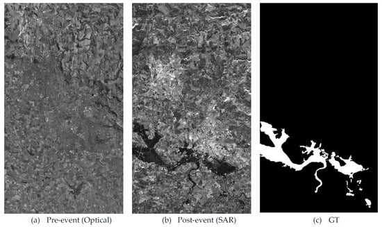
4.1. Image Pair 1: SAR-SPOT (Near Infrared)

This data set was the IEEE Contest data set [34]. The image size is 472 × 264 pixels. The event is flooding near Gloucester, UK. Figure 2 shows the pre- and post-event images. The pre-event image is a single band SAR (Figure 2a) and the post-event image is a near infrared (NIR) band of the SPOT image (Figure 2b). Figure 2c shows the ground truth (GT) change map.

Speckle filtering is a critical step before processing any SAR images especially when using them for change detection purposes. In this multimodal image pair, which the pre-event image is acquired by a SAR, we applied a Wiener filter for speckle filtering before applying the ten change detection algorithms. Figure 3 and Figure 4 show the ROC curves of ten algorithms without and with using EMAP, respectively. It can be seen that the performance variation is huge. We observe that IR, M3CD, CC, and HPT performed better than others. SSIM is the worst. We also observe that some methods have improved after using EMAP. For instance, HPT with EMAP was improved even further.

Table 2. Area under curve (AUC) values and differences between single band and EMAP cases for dataset-1. Bold numbers indicate the best performing method in each column. M3CD: Markov Model for Multimodal Change Detection; HPT: Homogeneous Pixel Transformation; D-MDS: Direct approach; T-MDS: Single band approach; CC: Chronochrome; CE: Covariance Equalization; ACD: Anomalous Change Detection; IR: Image Ratioing; PP: Pixel Pair; SSIM Structural Similarity.

Method	Single Band	EMAP	Difference
M3CD	0.927	0.9196	−0.0074
HPT	0.9801	0.9924	0.0123
D-MDS	0.6808	0.949	0.2682
T-MDS	0.8158	0.6119	−0.2039
CC	0.9154	0.9486	0.0332
ACD	0.7652	0.7897	0.0245
CE	0.419	0.4717	0.0527
IR	0.9921	0.9564	−0.0357
PP	0.7042	0.481	−0.2232
SSIM	0.2009	0.6482	0.4473

summarizes the AUC metrics. The last column of Table 2 shows the difference between the AUCs with EMAP and without EMAP. Positive numbers indicate improvements when using EMAP and negative numbers otherwise. It can be seen that six out of ten methods have benefitted from the use of EMAP.

Figure 5 compares the change maps produced by the various algorithms with and without using EMAP. Some change maps such as M3CD, HPT, CC, ACD, and IR look decent. However, CE, PP, and SSIM maps do not look that good. Moreover, change maps of T-MDS and PP appear to look worse with EMAP.

4.2. Image Pair 2: NIR-Optical

The image pair as shown in Figure 6 is between near infrared and optical where the pre-event image (Figure 6a) was captured with Landsat-5 Thermic (NIR band) and the post-event image (Figure 6b) was captured with optical imager. Figure 6c shows the ground truth. The image size is 412 × 300 pixels. The two images captured lake overfill after some rains. This pair was obtained from [26]. Only the greyscale images are available.

Figure 7 and Figure 8 show 20 ROC curves generated by ten algorithms without and with EMAP, respectively. It can be seen that HPT, IR, CC, and M3CD have good performance. SSIM and D-MDS are the worst. Since there are many curves, it is difficult to judge which methods have benefitted from the use of EMAP.

Table 3. AUC values and differences between single band and EMAP cases for dataset-2. Bold numbers indicate the best performing method in each column.

Method	Single Band	EMAP	Difference
M3CD	0.9363	0.9146	−0.0217
HPT	0.8798	0.9296	0.0498
D-MDS	0.5298	0.9312	0.4014
T-MDS	0.8851	0.8486	−0.0365
CC	0.9018	0.9164	0.0146
ACD	0.7531	0.7956	0.0425
CE	0.8309	0.848	0.0171
IR	0.9487	0.9292	−0.0195
PP	0.851	0.7993	−0.0517
SSIM	0.5753	0.2794	−0.2959

summarizes the AUC of all methods. Positive numbers in the last column indicate improved results and negative numbers correspond to worsening results. It can be observed that five methods have improved when EMAP was used. D-MDS improved the most from 0.53 to 0.93. SSIM suffered the most after using EMAP.

Figure 9 shows the change maps from all methods. M3CD and HPT have the cleanest change detection maps, followed by CC, ACD, IR, and CE. SSIM has the worst change map visually.

4.3. Image Pair 3: Optical-SAR

Here, the pre-event image (Figure 10a) is a QuickBird image and the post-event image (Figure 10b) is a TerraSAR-X image. The image size is 2325 × 4135. The ground truth change map is shown in Figure 10c. The event is flooding. This pair was obtained from [26]. Although Quickbird has four bands, only the grayscale image is available.

From the ROC curves shown in Figure 11 and Figure 12, one can observe that HPT and IR performed the best. D-MDS, T-MDS, ACD, CE, and SSIM did not perform well. In this dataset, it can be seen that quite a few methods with EMAP have improved significantly over those without EMAP.

To quantify the performance gain of using EMAP, one can look at

Table 4. AUC values and differences between single band and EMAP cases for dataset-3. Bold numbers indicate the best performing method in each column.

Method	Single Band	EMAP	Difference
M3CD	0.9042	0.9098	0.0056
HPT	0.847	0.9427	0.0957
D-MDS	0.5052	0.539	0.0338
T-MDS	0.5383	0.6157	0.0774
CC	0.8394	0.8812	0.0418
ACD	0.5135	0.4901	−0.0234
CE	0.6631	0.7416	0.0785
IR	0.8624	0.9395	0.0771
PP	0.7209	0.7472	0.0263
SSIM	0.6023	0.5822	−0.0201

. We can see that eight out of ten methods have benefitted from the use of EMAP. The HPT method increased from 0.847 to 0.9427, which is quite significant.

Figure 13 compares the change maps of all methods. It can be seen that HPT looks cleaner and has fewer false alarms. The IR and M3CD results also look decent. The change map of CC with EMAP has improved over that without EMAP. Other methods do not seem to yield good results.

4.4. Image Pair 4: SAR-Optical

This pair was obtained from [26]. As shown in Figure 14, the pre-event image is a TerraSAR-X image (Figure 14a) and the post-event image (Figure 14b) is an optical image from Pleiades. The ground truth change map is shown in Figure 14c. The image size is 4404 × 2604. The objective is to detect changes due to construction. Only the grayscale image (Pleiades) was available.

From the ROC curves shown in Figure 15 and Figure 16, we can see that M3CD and CC performed better than others. Others did not perform well. It appears that the pre-event SAR image is quite noisy. However, some filtering operations such as median filtering did not enhance the performance any further. The methods with EMAP have seen dramatic improvements. For instance, HPT with EMAP (dotted red) improved quite a lot over the case of without EMAP (red). The D-MDS method suffered some drawback when EMAP was used.

Table 5. AUC values and differences between single band and EMAP cases for dataset-4. Bold numbers indicate the best performing method in each column.

Method	Single Band	EMAP	Difference
M3CD	0.8328	0.841	0.0082
HPT	0.6373	0.8637	0.2264
D-MDS	0.4995	0.171	−0.3285
T-MDS	0.5327	0.4309	−0.1018
CC	0.7243	0.7761	0.0518
ACD	0.4491	0.5026	0.0535
CE	0.66	0.6917	0.0317
IR	0.7093	0.7289	0.0196
PP	0.6569	0.6851	0.0282
SSIM	0.5437	0.4826	−0.0611

summarizes the AUC values of all the methods. One can see that seven out of ten methods have seen improvements when EMAP was used. HPT received the most performance boost.

Figure 17 compares the change maps of all the methods with and without EMAP. We can see that M3CD, HPT, CC, IR, CE, and PP have relatively clean change maps. However, D-MDS, T-MDS, and SSIM methods do not have clean change maps.

4.5. Image Pair 5: Optical-Optical

This is an optical pair with only grayscale images. This pair was obtained from [26]. As shown in Figure 18, the pre-event image (Figure 18a) was captured with Pleiades and the post-event image (Figure 18b) was captured with Worldview 2. Figure 18c shows the ground truth change map. The image size is 2000 × 2000. The grey images are formed by taking the average of several bands. The band compositions are different in the pre- and post-event images. Since the spectral bands in the two images are different, the appearance of the two images are quite different, making this pair very difficult for change detection. The objective of the change detection is to capture construction activities.

From the ROC curves in Figure 19 and Figure 20, M3CD was the best. SSIM also performed well perhaps due to the fact this pair is an optical-optical image pair. SSIM is likely to work better for homogeneous images. D-MDS, T-MDS, ACD, CE, IR, and PP did not work well. We can also see that some methods with EMAP such as HPT have seen performance improvements.

Table 6. AUC values and differences between single band and EMAP cases for dataset-5. Bold numbers indicate the best performing method in each column.

Method	Single Band	EMAP	Difference
M3CD	0.804	0.8128	0.0088
HPT	0.5163	0.6926	0.1763
D-MDS	0.2807	0.2316	−0.0491
T-MDS	0.3796	0.5688	0.1892
CC	0.5631	0.5837	0.0206
ACD	0.5115	0.5135	0.002
CE	0.5588	0.5797	0.0209
IR	0.488	0.5016	0.0136
PP	0.5598	0.5925	0.0327
SSIM	0.7961	0.6404	−0.1557

summarizes all the AUC values of the methods with and without EMAP. It is very clear to see that eight out of ten methods have seen improved performance. The HPT method improved from 0.52 to 0.69. It is also observed that SSIM suffered some setback when EMAP was used.

Figure 21 compares the change maps of all methods with and without EMAP. M3CD has the best visual performance. HPT with EMAP also has good change detection map. Others do not have distinct change detection. It can be seen that SSIM map is somewhat fuzzy, but nevertheless captures most of the changes.

5. Observations

To quantify the performance gain, the AUC measure was applied to the resultant ROC curves of all methods for the two change detection cases (using the original single band and using EMAP-synthetic bands) to assess the impact of using EMAP synthetic bands for change detection. The EMAP results for a change detection method are then compared with the corresponding reference case (that uses original single band) of the same change detection method. The AUC differences for the reference and EMAP cases are used as a measure to assess how EMAP affects the performance of a change detection method.

Table 7. AUC Differences between using single band case and using EMAP-synthetic bands for change detection.

Method	Dataset-1 (SAR-SPOT)	Dataset-2 (Montreal-1)	Dataset-3 (Montreal-5)	Dataset-4 (Montreal-6)	Dataset-5 (Montreal-7)
M3CD	−0.0074	−0.0217	0.0056	0.0082	0.0088
HPT	0.0123	0.0498	0.0957	0.2264	0.1763
D-MDS	0.2682	0.4014	0.0338	−0.3285	−0.0491
T-MDS	−0.2039	−0.0365	0.0774	−0.1018	0.1892
CC	0.0332	0.0146	0.0418	0.0518	0.0206
ACD	0.0245	0.0425	−0.0234	0.0535	0.002
CE	0.0527	0.0171	0.0785	0.0317	0.0209
IR	−0.0357	−0.0195	0.0771	0.0196	0.0136
PP	−0.2232	−0.0517	0.0263	0.0282	0.0327
SSIM	0.4473	−0.2959	−0.0201	−0.0611	−0.1557

shows the AUC differences between using original single band case and using EMAP-synthetic bands for change detection. The positive-valued cells in Table 7 indicate that using EMAP-synthetic bands improved the detection performance and negative-valued cells indicate that it degraded the detection performance for that method. Overall, it is observed that the change detection performances of many of the applied change detection methods are improved by using the EMAP synthetic bands. A very consistent detection performance boost in all five datasets was observed for HPT, CC, and CE methods. Especially, HPT tends to be significantly improved by using EMAP bands except in the dataset-1 where it already performs well. Similarly, detection performance was improved for the ACD method in four of the five datasets. The only dataset where ACD’s performance slightly decreased is the third dataset. M3CD is affected slightly by using the EMAP bands since in most datasets the ROC curves are very close to each other for original single band case and EMAP case. Image Ratio, Pixel Pair, D-MDS and T-MDS results with EMAP are found to be inconsistent. In some datasets, these methods perform better and in some worse using EMAP showing no clear pattern. SSIM tends to perform worse with the EMAP synthetic bands with the exception of the first dataset.

The computational complexity of the ten algorithms varies quite a lot.

Table 8. Comparison of computational times of the ten algorithms for Dataset-1.

	Time (s) with Single Band	Time (s) with EMAP
M3CD	2024	22504
HPT	4989	5497
CC	34	53
ACD	8	9
CE	27	44
D-MDS	6	45
T-MDS	123	125
IR	3	27
PP	486	6742
SSIM	185	1731

summarizes the processing times of different algorithms with and without using EMAP for Dataset-1. The algorithms, excluding M3CD, were run using a computer (Windows 7) with an Intel Pentium CPU with 2.90 GHz, 2 Cores, and 4 GB of RAM. The M3CD algorithm was executed in a Linux computer with Intel i7-4790 CPU at 3.60 GHz and 24 GB of RAM.

It can be seen that HPT is the most time-consuming algorithm, followed by M3CD and PP. CC, ACD, CE, IR, and D-MDS are all low complexity algorithms.

6. Conclusions

In this paper, we investigated the use of EMAP to generate synthetic bands and examined the impact of EMAP use in change detection performance using heterogeneous images. We presented extensive comparative studies with ten change detection algorithms (nine of them from the literature and one of our own) using five multimodal datasets. From the investigations, we observed that, in 34 out of 50 cases, change detection performance was improved, which shows a strong indication about the positive impact of using EMAP for change detection, especially when the number of original bands in the image pair is not that many. A consistent change detection performance boost in all five datasets was observed with the use of EMAP for HPT, CC, and CE.