Large-Scale Mode Impacts on the Sea Level over the Red Sea and Gulf of Aden

 ,
,  , and
, and
Abstract
:
1. Introduction
2. Data and Methods
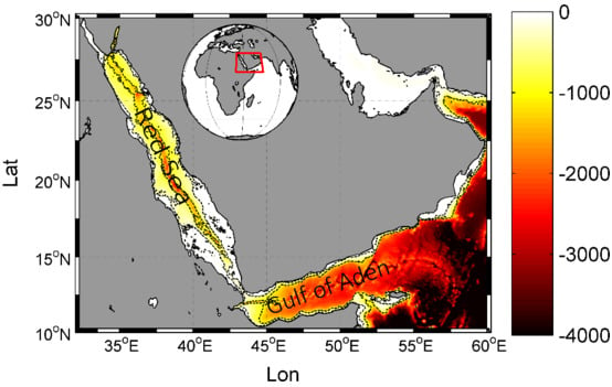
2.1. Study Area
2.2. Data
2.3. Methods
3. Results
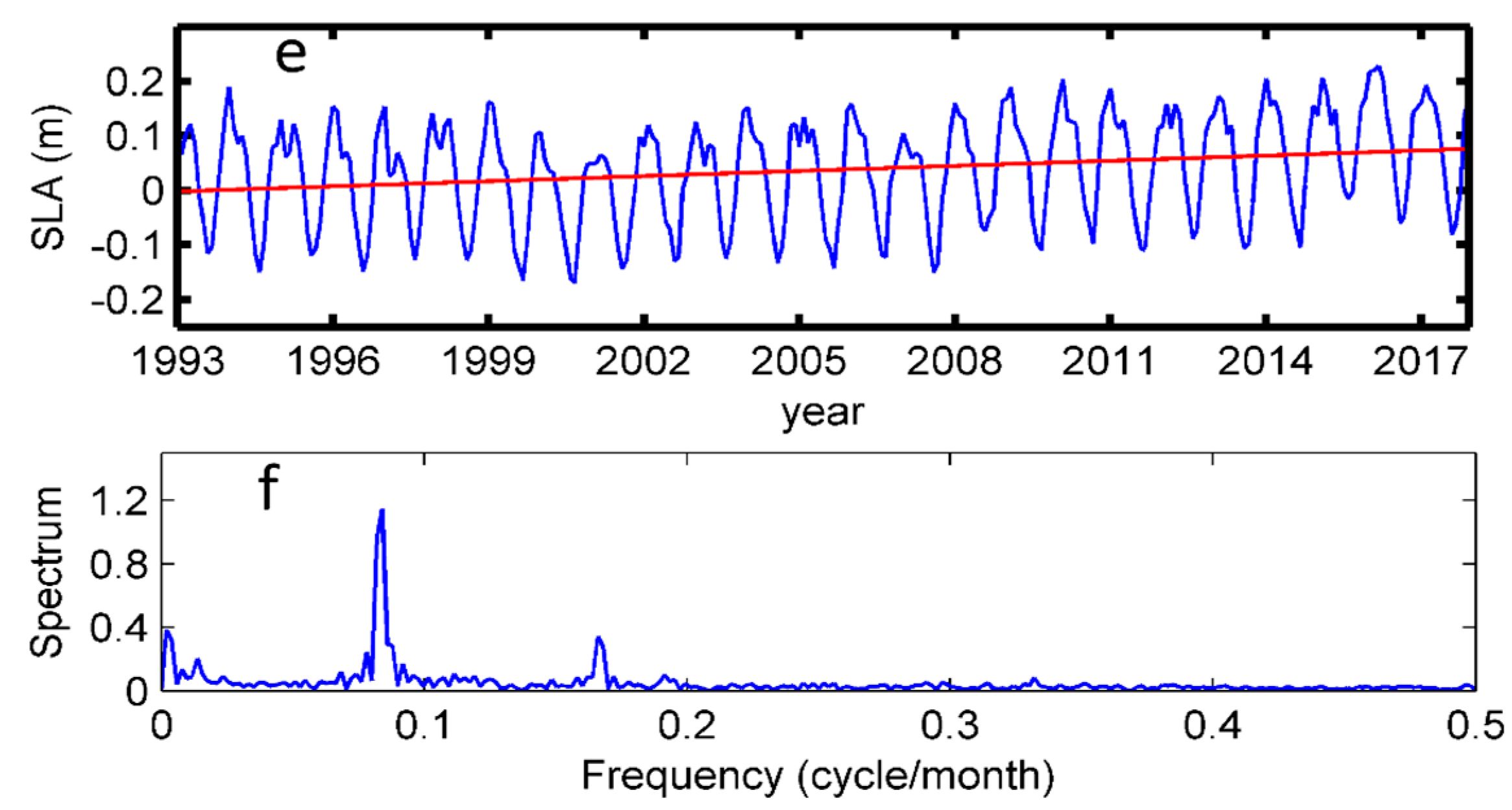
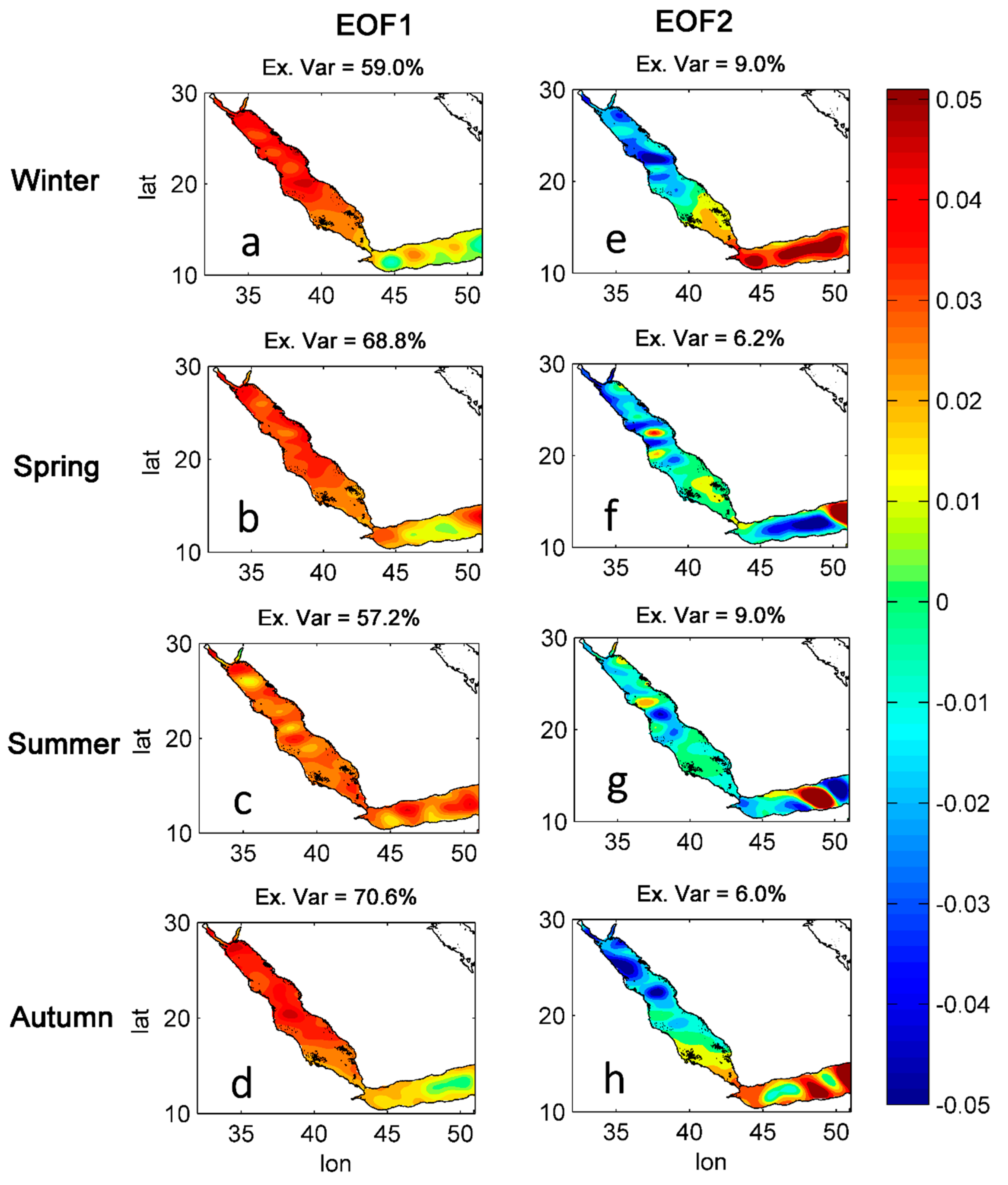
3.1. The SLA Trend and the Dominant Modes
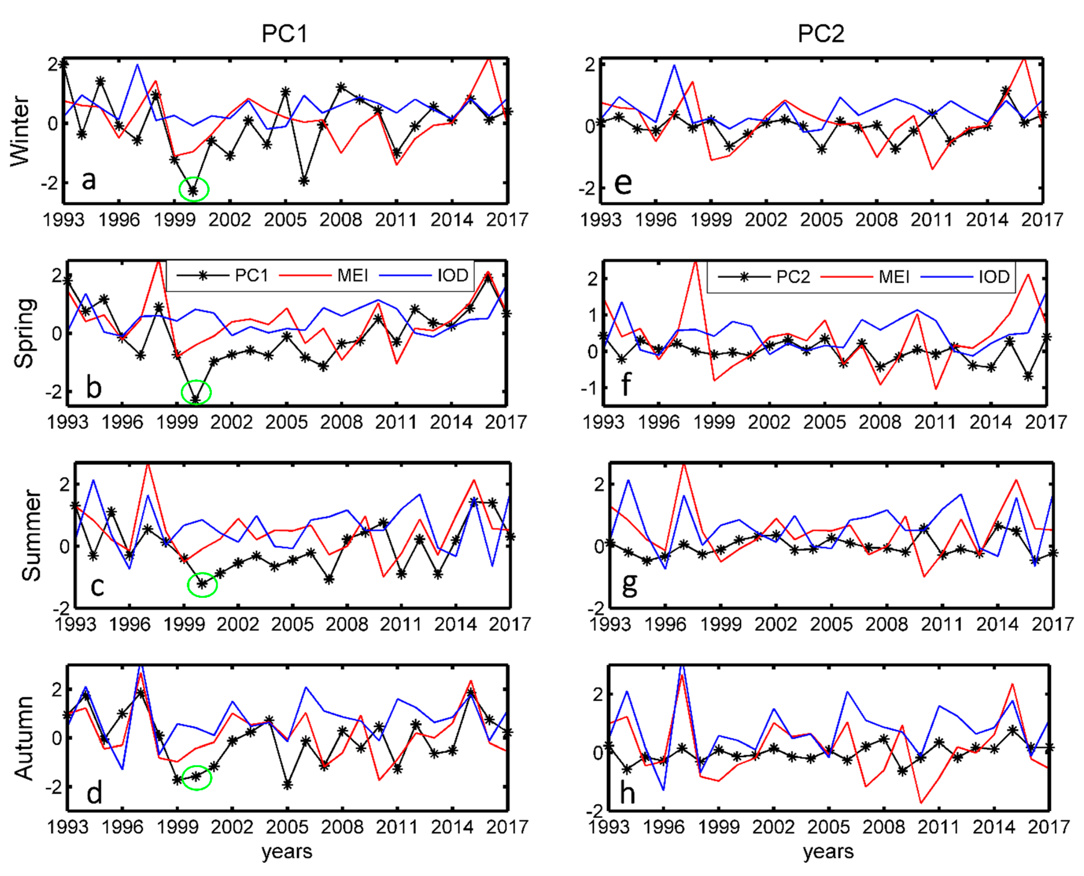
3.2. Link between the SLA and Large-Scale Modes
3.3. The Physical Mechanisms
3.3.1. The Relation with SLA, Wind and 20 °C isotherm in the IO
3.3.2. The Relationship with Global Temperature
4. Discussion
5. Conclusions
- the SLA reflects the annual and semi-annual cycle, which agrees with previous studies;
- the first leading mode throughout the seasons explained, on average, about 65% of the total variance, while their PCs clearly capture the strong La Niña event (1999–2001) during all seasons; and,
- the SLA showed a strong positive relation with ENSO during all seasons and a strong negative relation with EAWR during winter and spring.
Author Contributions
Funding
Acknowledgments
Conflicts of Interest
References
- Church, J.A.; White, N.J. A 20th century acceleration in global sea-level rise. Geophys. Res. Lett. 2006, 33, 33. [Google Scholar] [CrossRef]
- Church, J.A.; White, N.J. Sea-level rise from the late 19th to the early 21st century. Surv. Geophys. 2011, 32, 585–602. [Google Scholar] [CrossRef]
- Church, J.A.; Clark, P.U.; Cazenave, A.; Gregory, J.M.; Jevrejeva, S.; Levermann, A.; Merrifield, M.A.; Milne, G.A.; Nerem, R.S.; Nunn, P.D.; et al. Sea level change. Climate change 2013: The physical science basis. In Contribution of Working Group I to the Fifth Assessment Report of the Intergovernmental Panel on Climate Change; Cambridge University Press: Cambridge, UK; New York, NY, USA, 2013; pp. 1137–1216. [Google Scholar]
- Pachauri, R.K.; Allen, M.R.; Barros, V.R.; Broome, J.; Cramer, W.; Christ, R.; Church, J.A.; Clarke, L.; Dahe, Q.; Dasgupta, P.; et al. Climate change 2014: Synthesis report. In Contribution of Working Groups I, Ii and Iii to the Fifth Assessment Report of the Intergovernmental Panel on Climate Change; IPCC: Geneva, Switzerland, 2014. [Google Scholar]
- Katsman, C.A.; Hazeleger, W.; Drijfhout, S.S.; van Oldenborgh, G.J.; Burgers, G. Climate scenarios of sea level rise for the northeast Atlantic Ocean: A study including the effects of ocean dynamics and gravity changes induced by ice melt. Clim. Chang. 2008, 91, 351–374. [Google Scholar] [CrossRef]
- Stammer, D.; Cazenave, A.; Ponte, R.M.; Tamisiea, M.E. Causes for contemporary regional sea level changes. Annu. Rev. Mar. Sci. 2013, 5, 21–46. [Google Scholar] [CrossRef]
- Carson, M.; Köhl, A.; Stammer, D.; Slangen, A.B.A.; Katsman, C.A.; Van de Wal, R.S.W.; Church, J.; White, N. Coastal sea level changes, observed and projected during the 20th and 21st century. Clim. Chang. 2016, 134, 269–281. [Google Scholar] [CrossRef]
- Cui, M.; STORCH, H.V.; Zorita, E. Coastal sea level and the large-scale climate state A downscaling exercise for the Japanese Islands. Tellus A 1995, 47, 132–144. [Google Scholar] [CrossRef]
- Nerem, R.S.; Chambers, D.P.; Leuliette, E.W.; Mitchum, G.T.; Giese, B.S. Variations in global mean sea level associated with the 1997–1998 ENSO event: Implications for measuring long term sea level change. Geophys. Res. Lett. 1999, 26, 3005–3008. [Google Scholar] [CrossRef]
- Antonov, J.I.; Levitus, S.; Boyer, T.P. Thermosteric sea level rise. Geophys. Res. Lett. 2005, 32, 1955–2003. [Google Scholar]
- Landerer, F.W.; Jungclaus, J.H.; Marotzke, J. El Niño–Southern Oscillation signals in sea level, surface mass redistribution, and degree-two geoid coefficients. J. Geophys. Res. Space Phys. 2008, 113. [Google Scholar] [CrossRef]
- Moon, J.H.; Song, Y.T.; Lee, H. PDO and ENSO modulations intensified decadal sea level variability in the tropical Pacific. J. Geophys. Res. Ocean. 2015, 120, 8229–8237. [Google Scholar] [CrossRef]
- Hamlington, B.D.; Cheon, S.H.; Thompson, P.R.; Merrifield, M.A.; Nerem, R.S.; Leben, R.R.; Kim, K.-Y.; Kim, K. An ongoing shift in Pacific Ocean sea level. J. Geophys. Res. Ocean. 2016, 121, 5084–5097. [Google Scholar] [CrossRef] [Green Version]
- Piecuch, C.G.; Quinn, K.J. El Niño, La Niña, and the global sea level budget. Ocean. Sci. 2016, 12, 1165–1177. [Google Scholar] [CrossRef]
- Nidheesh, A.G.; Lengaigne, M.; Vialard, J.; Izumo, T.; Unnikrishnan, A.S.; Meyssignac, B.; Hamlington, B.; Montegut, C.D.B.; Montegut, C.B. Robustness of observation-based decadal sea level variability in the Indo-Pacific Ocean. Geophys. Res. Lett. 2017, 44, 7391–7400. [Google Scholar] [CrossRef] [Green Version]
- Arpe, K.; Bengtsson, L.; Golitsyn, G.S.; Mokhov, I.I.; Semenov, V.A.; Sporyshev, P.V. Connection between Caspian Sea level variability and ENSO. Geophys. Res. Lett. 2000, 27, 2693–2696. [Google Scholar] [CrossRef]
- Stanev, E.V.; Peneva, E.L. Regional sea level response to global climatic change: Black Sea examples. Glob. Planet. Chang. 2001, 32, 33–47. [Google Scholar] [CrossRef]
- Zanchettin, D.; Rubino, A.; Traverso, P.; Tomasino, M. Teleconnections force interannual-to-decadal tidal variability in the Lagoon of Venice (northern Adriatic). J. Geophys. Res. Space Phys. 2009, 114. [Google Scholar] [CrossRef]
- Calafat, F.M.; Chambers, D.P.; Tsimplis, M.N. Mechanisms of decadal sea level variability in the eastern North Atlantic and the Mediterranean Sea. J. Geophys. Res. Space Phys. 2012, 117. [Google Scholar] [CrossRef]
- Tsimplis, M.N.; Calafat, F.M.; Marcos, M.; Jorda, G.; Gomis, D.; Fenoglio-Marc, L.; Struglia, M.V.; Josey, S.A.; Chambers, D. The effect of the NAO on sea level and on mass changes in the Mediterranean Sea. J. Geophys. Res. Space Phys. 2013, 118, 944–952. [Google Scholar] [CrossRef] [Green Version]
- Patzert, W.C. Wind-induced reversal in Red Sea circulation. Deep. Sea Res. Oceanogr. Abstr. 1974, 21, 109–121. [Google Scholar] [CrossRef]
- Sultan, S.A.R.; Ahmad, F.; El-Hassan, A. Seasonal variations of the sea level in the central part of the Red Sea. Estuar. Coast. Shelf Sci. 1995, 40, 1–8. [Google Scholar] [CrossRef]
- Sultan, S.A.R.; Ahmad, F.; Nassar, D. Relative contribution of external sources of mean sea-level variations at Port Sudan, Red Sea. Estuar. Coast. Shelf Sci. 1996, 42, 19–30. [Google Scholar] [CrossRef]
- Sofianos, S.S.; Johns, W.E. Wind induced sea level variability in the Red Sea. Geophys. Res. Lett. 2001, 28, 3175–3178. [Google Scholar] [CrossRef]
- Sultan, S.A.R.; Elghribi, N.M. Sea Level Changes in the Central Part of the Red Sea; CSIR: New Delhi, India, 2003. [Google Scholar]
- Manasrah, R.; Hasanean, H.M.; Al-Rousan, S. Spatial and seasonal variations of sea level in the Red Sea, 1958–2001. Ocean Sci. J. 2009, 44, 145–159. [Google Scholar] [CrossRef]
- Alawad, K.; Alsaafani, M.A.; Al-Subhi, A.M.; Alraddadi, T.M. Signatures of Tropical Climate Modes on the Red Sea and Gulf of Aden Sea Level; NISCAIR-CSIR: New Delhi, India, 2017. [Google Scholar]
- Al-Rousan, S.; Al-Moghrabi, S.; Pätzold, J.; Wefer, G. Environmental and biological effects on the stable oxygen isotope records of corals in the northern Gulf of Aqaba, Red Sea. Mari. Ecol. Prog. Ser. 2002, 239, 301–310. [Google Scholar] [CrossRef]
- Al-Rousan, S.; Al-Moghrabi, S.; Pätzold, J.; Wefer, G. Stable oxygen isotopes in Porites corals monitor weekly temperature variations in the northern Gulf of Aqaba, Red Sea. Coral Reefs 2003, 22, 346–356. [Google Scholar] [CrossRef]
- Arz, H.W.; Lamy, F.; Pätzold, J.; Müller, P.J.; Prins, M. Mediterranean moisture source for an Early-Holocene humid period in the northern Red Sea. Science 2003, 300, 118–121. [Google Scholar] [CrossRef] [PubMed]
- Al-Rousan, S.; Felis, T.; Manasrah, R.; Al-Horani, F. Seasonal variations in the stable oxygen isotopic composition in Porites corals from the northern Gulf of Aqaba, Red Sea. Geochem. J. 2007, 41, 333–340. [Google Scholar] [CrossRef] [Green Version]
- Felis, T.; Pätzold, J.; Loya, Y.; Fine, M.; Nawar, A.H.; Wefer, G. A coral oxygen isotope record from the northern Red Sea documenting NAO, ENSO, and North Pacific teleconnections on Middle East climate variability since the year 1750. Paleoceanogr. Paleoclimatology 2000, 15, 679–694. [Google Scholar] [CrossRef]
- Rimbu, N.; Lohmann, G.; Felis, T.; Pätzold, J. Arctic Oscillation signature in a Red Sea coral. Geophys. Res. Lett. 2001, 28, 2959–2962. [Google Scholar] [CrossRef] [Green Version]
- Ionita, M.; Felis, T.; Lohmann, G.; Rimbu, N.; Pätzold, J. Distinct modes of East Asian Winter Monsoon documented by a southern Red Sea coral record. J. Geophys. Res. Space Phys. 2014, 119, 1517–1533. [Google Scholar] [CrossRef] [Green Version]
- Papadopoulos, V.P.; Abualnaja, Y.; Josey, S.A.; Bower, A.; Raitsos, D.E.; Kontoyiannis, H.; Hoteit, I. Atmospheric forcing of the winter air–sea heat fluxes over the northern Red Sea. J. Clim. 2013, 26, 1685–1701. [Google Scholar] [CrossRef]
- Abualnaja, Y.; Papadopoulos, V.P.; Josey, S.A.; Hoteit, I.; Kontoyiannis, H.; Raitsos, D.E. Impacts of climate modes on air–sea heat exchange in the Red Sea. J. Clim. 2015, 28, 2665–2681. [Google Scholar] [CrossRef]
- Morcos, S.A. Physical and chemical oceanography of the Red Sea. Oceanogr. Mar. Biol. Annu. Rev. 1970, 8, 73–202. [Google Scholar]
- Al Saafani, M.A.; Shenoi, S.S.C. Water masses in the Gulf of Aden. J. Oceanogr. 2007, 63, 1–14. [Google Scholar] [CrossRef]
- Dee, D.P.; Uppala, S.M.; Simmons, A.J.; Berrisford, P.; Poli, P.; Kobayashi, S.; Andrae, U.; Balmaseda, M.A.; Balsamo, G.; Bauer, P. The ERA-Interim reanalysis: Configuration and performance of the data assimilation system. Q. J. R. Meteorol. Soc. 2011, 137, 553–597. [Google Scholar] [CrossRef]
- Lorenz, E.N. Empirical Orthogonal Functions and Statistical Weather Prediction; Massachusetts Institute of Technology: Cambridge, MA, USA, 1956. [Google Scholar]
- Björnsson, H.; Venegas, S.A. A manual for EOF and SVD analyses of climatic data. CCGCR Rep. 1997, 97, 112–134. [Google Scholar]
- Currie, J.C.; Lengaigne, M.; Vialard, J.; Kaplan, D.M.; Aumont, O.; Naqvi, S.W.A.; Maury, O. Indian Ocean dipole and El Nino/southern oscillation impacts on regional chlorophyll anomalies in the Indian Ocean. Biogeosciences 2013, 10, 6677–6698. [Google Scholar] [CrossRef]
- Saji, N.H.; Xie, S.P.; Yamagata, T. Tropical Indian Ocean variability in the IPCC twentieth-century climate simulations. J. Clim. 2006, 19, 4397–4417. [Google Scholar] [CrossRef]
- Klein, S.A.; Soden, B.J.; Lau, N.-C. Remote sea surface temperature variations during ENSO: Evidence for a tropical atmospheric bridge. J. Clim. 1999, 12, 917–932. [Google Scholar] [CrossRef]
- Saji, N.H.; Yamagata, T. Structure of SST and surface wind variability during Indian Ocean dipole mode events: COADS observations. J. Clim. 2003, 16, 2735–2751. [Google Scholar] [CrossRef]
- Du, Y.; Xie, S.-P.; Huang, G.; Hu, K. Role of air–sea interaction in the long persistence of El Niño–induced north Indian Ocean warming. J. Clim. 2009, 22, 2023–2038. [Google Scholar] [CrossRef]
- Alexander, M.A.; Bladé, I.; Newman, M.; Lanzante, J.R.; Lau, N.-C.; Scott, J.D. The atmospheric bridge: The influence of ENSO teleconnections on air–sea interaction over the global oceans. J. Clim. 2002, 15, 2205–2231. [Google Scholar] [CrossRef]
- Raitsos, D.E.; Yi, X.; Platt, T.; Racault, M.-F.; Pradhan, Y.; Papadopoulos, V.; Sathyendranath, S.; Hoteit, I.; Brewin, R.J.W. Monsoon oscillations regulate fertility of the Red Sea. Geophys. Res. Lett. 2015, 42, 855–862. [Google Scholar] [CrossRef] [Green Version]
- Liu, L.; Feng, L.; Wu, Y.; Yu, W.; Liu, L.; Yang, G.; Han, G. Why was the Indian Ocean dipole weak in the context of the extreme El Niño in 2015? J. Clim. 2017, 30, 4755–4761. [Google Scholar] [CrossRef]
- Xie, S.P.; Annamalai, H.; Schott, F.A.; McCreary, J.P. Structure and mechanisms of South Indian Ocean climate variability. J. Clim. 2002, 15, 864–878. [Google Scholar] [CrossRef]
- Fan, L.; Liu, Q.; Wang, C.; Guo, F. Indian Ocean dipole modes associated with different types of ENSO development. J. Clim. 2017, 30, 2233–2249. [Google Scholar] [CrossRef]
- Webster, P.J.; Yang, S. Monsoon and ENSO: Selectively interactive systems. Q. J. R. Meteorol. Soc. 1992, 118, 877–926. [Google Scholar] [CrossRef]
- Lau, K.M.; Yang, S. The Asian monsoon and predictability of the tropical ocean–atmosphere system. Q. J. R. Meteorol. Soc. 1996, 122, 945–957. [Google Scholar]
- Shanas, P.R.; Aboobacker, V.M.; Albarakati, A.M.; Zubier, K.M. Climate driven variability of wind-waves in the Red Sea. Ocean Model. 2017, 119, 105–117. [Google Scholar] [CrossRef]
- Karnauskas, K.B.; Jones, B.H. The interannual variability of sea surface temperature in the Red Sea from 35 years of satellite and in situ observations. J. Geophys. Res. Oceans 2018, 123, 5824–5841. [Google Scholar] [CrossRef]
- Tourre, Y.M.; White, W.B. ENSO signals in global upper-ocean temperature. J. Phys. Oceanogr. 1995, 25, 1317–1332. [Google Scholar] [CrossRef]
- Yu, L.; Rienecker, M.M. Mechanisms for the Indian Ocean warming during the 1997–98 El Nino. Geophys. Res. Lett. 1999, 26, 735–738. [Google Scholar] [CrossRef]
- Abish, B.; Cherchi, A.; Ratna, S.B. ENSO and the recent warming of the Indian Ocean: ENSO AND THE INDIAN OCEAN WARMING. Int. J. Climatol. 2018, 38, 203–214. [Google Scholar] [CrossRef]
- Chambers, D.P.; Tapley, B.D.; Stewart, R.H. Anomalous warming in the Indian Ocean coincident with El Nino. J. Geophys. Res. Ocean. 1999, 104, 3035–3047. [Google Scholar] [CrossRef]
- Salim, M.; Nayak, R.K.; Swain, D.; Dadhwal, V.K. Sea surface height variability in the tropical Indian Ocean: Steric contribution. J. Indian Soc. Remote. Sens. 2012, 40, 679–688. [Google Scholar] [CrossRef]
- Liu, Y.; Wang, L.; Zhou, W.; Chen, W. Three Eurasian teleconnection patterns: Spatial structures, temporal variability, and associated winter climate anomalies. Clim. Dyn. 2014, 42, 2817–2839. [Google Scholar] [CrossRef]
- Cai, W.; Borlace, S.; Lengaigne, M.; Van Rensch, P.; Collins, M.; Vecchi, G.; Timmermann, A.; Santoso, A.; McPhaden, M.J.; Wu, L.; et al. Increasing frequency of extreme El Niño events due to greenhouse warming. Nat. Clim. Chang. 2014, 4, 111–116. [Google Scholar] [CrossRef]
- Terray, P.; Dominiak, S. Indian Ocean sea surface temperature and El Niño–Southern Oscillation: A new perspective. J. Clim. 2005, 18, 1351–1368. [Google Scholar] [CrossRef]
- Terray, P.; Delécluse, P.; Labattu, S.; Terray, L. Sea surface temperature associations with the late Indian summer monsoon. Clim. Dyn. 2003, 21, 593–618. [Google Scholar] [CrossRef] [Green Version]
- Wang, B.; An, S.I. Why the properties of El Niño changed during the late 1970s. Geophys. Res. Lett. 2001, 28, 3709–3712. [Google Scholar] [CrossRef]
- Ding, R.; Ha, K.J.; Li, J. Interdecadal shift in the relationship between the East Asian summer monsoon and the tropical Indian Ocean. Clim. Dyn. 2010, 34, 1059–1071. [Google Scholar] [CrossRef]
- Nakamura, N.; Kayanne, H.; Iijima, H.; McClanahan, T.R.; Behera, S.K.; Yamagata, T. Mode shift in the Indian Ocean climate under global warming stress. Geophys. Res. Lett. 2009, 36. [Google Scholar] [CrossRef]
- Sofianos, S.S.; Johns, W.E. An oceanic general circulation model (OGCM) investigation of the Red Sea circulation: 2. Three-dimensional circulation in the Red Sea. J. Geophys. Res. Space Phys. 2003, 108. [Google Scholar] [CrossRef]


| Name | Abbreviation | Sources |
|---|---|---|
| MEI | Multivariate El Niño Index | https://www.esrl.noaa.gov/psd/enso/mei/table.html |
| IOD | Indian Ocean Dipole | https://www.esrl.noaa.gov/psd/gcos_wgsp/Timeseries/Data/dmi.long.data |
| EAWR | East Atlantic-West Russian | ftp://ftp.cpc.ncep.noaa.gov/wd52dg/data/indices/eawr_index.tim |
| EOF PCs | IOD | MEI | EAWR |
|---|---|---|---|
| PC1 winter | 0.36 (0.076) | 0.39 (0.056) | –0.40 |
| PC1 spring | 0.66 | –0.47 | |
| PC1 summer | 0.46 | ||
| PC1 autumn | 0.57 | ||
| PC2 winter | |||
| PC2 spring | |||
| PC2 summer | |||
| PC2 autumn |
© 2019 by the authors. Licensee MDPI, Basel, Switzerland. This article is an open access article distributed under the terms and conditions of the Creative Commons Attribution (CC BY) license (http://creativecommons.org/licenses/by/4.0/).
Share and Cite
Alawad, K.A.; Al-Subhi, A.M.; Alsaafani, M.A.; Alraddadi, T.M.; Ionita, M.; Lohmann, G. Large-Scale Mode Impacts on the Sea Level over the Red Sea and Gulf of Aden. Remote Sens. 2019, 11, 2224. https://doi.org/10.3390/rs11192224
Alawad KA, Al-Subhi AM, Alsaafani MA, Alraddadi TM, Ionita M, Lohmann G. Large-Scale Mode Impacts on the Sea Level over the Red Sea and Gulf of Aden. Remote Sensing. 2019; 11(19):2224. https://doi.org/10.3390/rs11192224
Chicago/Turabian StyleAlawad, Kamal A., Abdullah M. Al-Subhi, Mohammed A. Alsaafani, Turki M. Alraddadi, Monica Ionita, and Gerrit Lohmann. 2019. "Large-Scale Mode Impacts on the Sea Level over the Red Sea and Gulf of Aden" Remote Sensing 11, no. 19: 2224. https://doi.org/10.3390/rs11192224