High-Frequency Variations in Pearl River Plume Observed by Soil Moisture Active Passive Sea Surface Salinity

 and
and 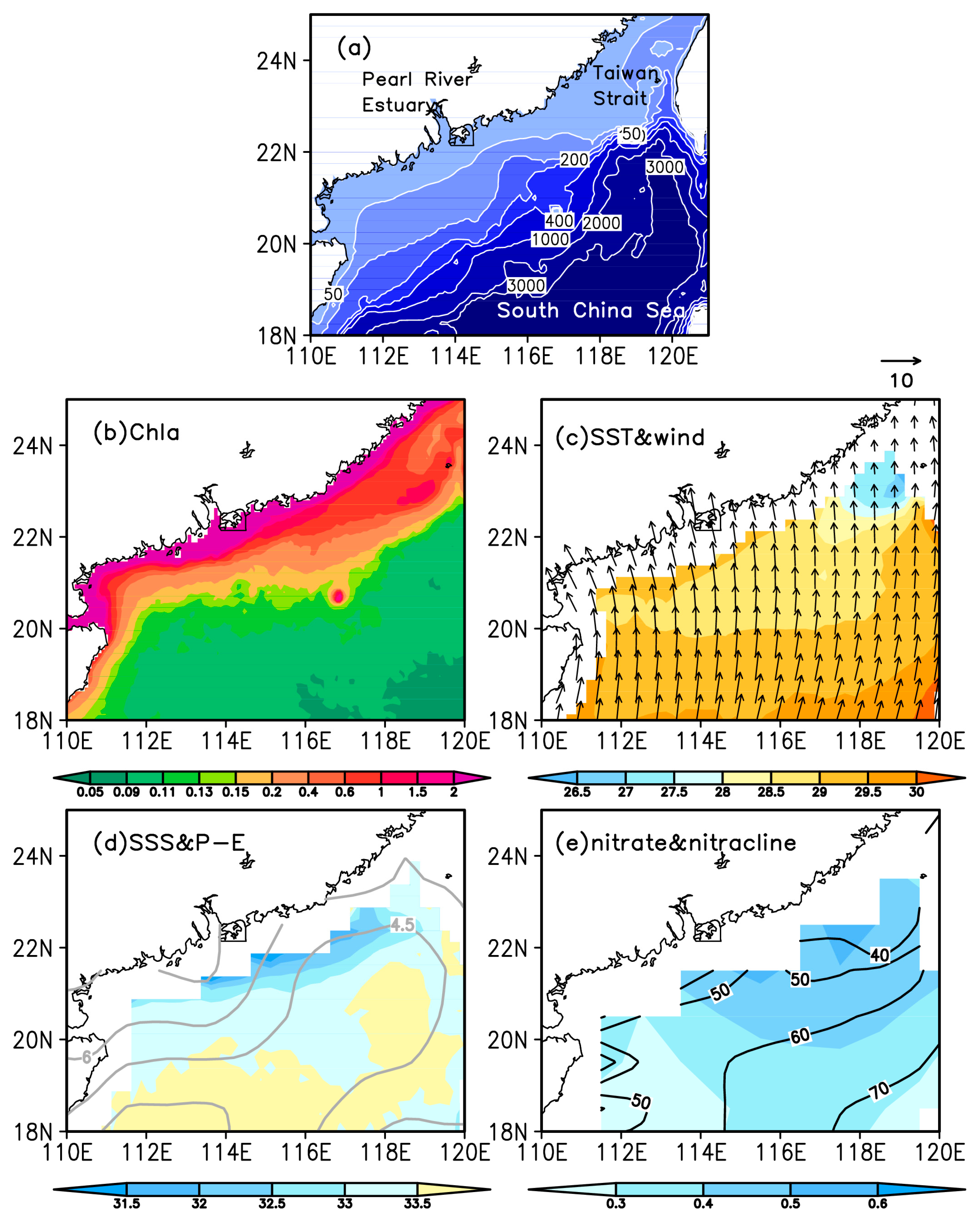
Abstract
:1. Introduction
2. Data and Methods
3. Results and discussion
3.1. General Features
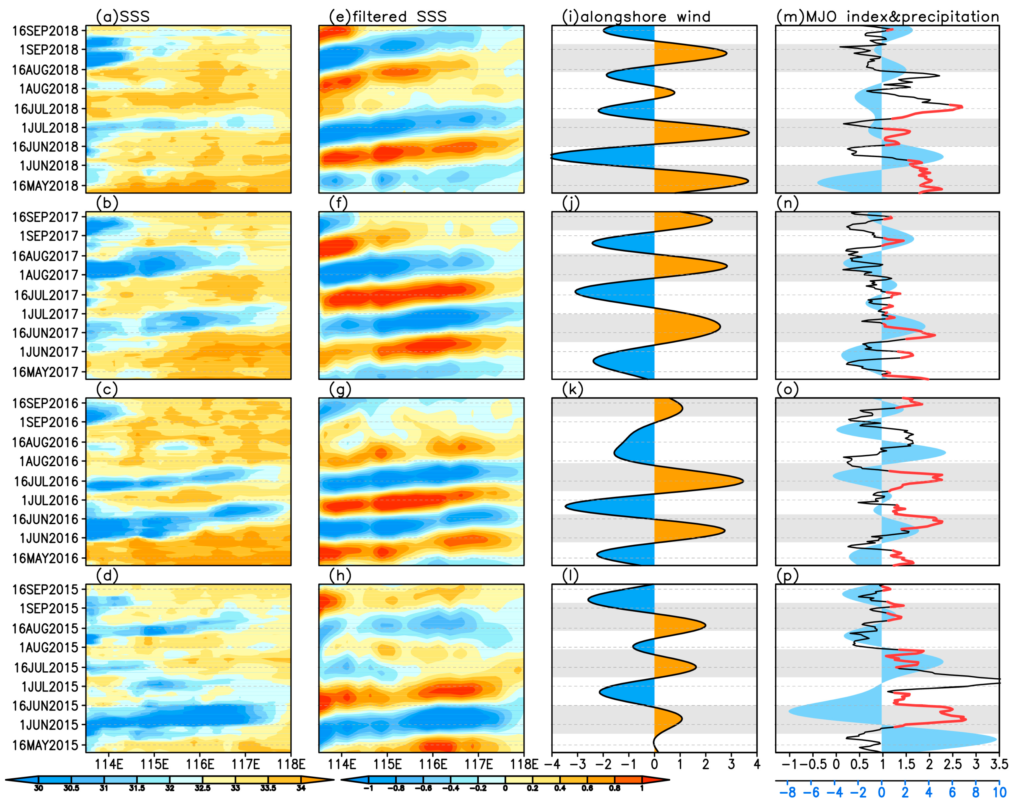
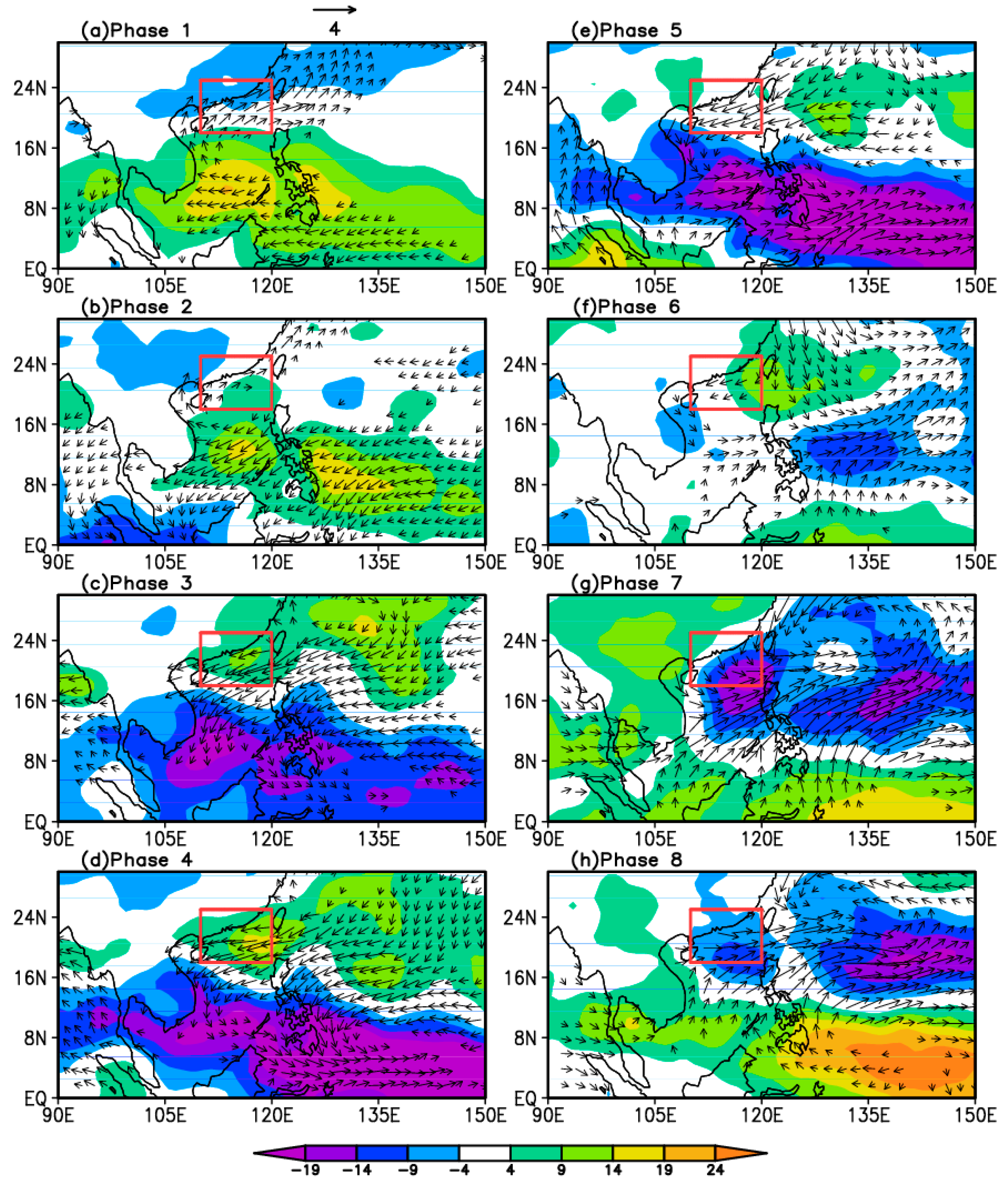
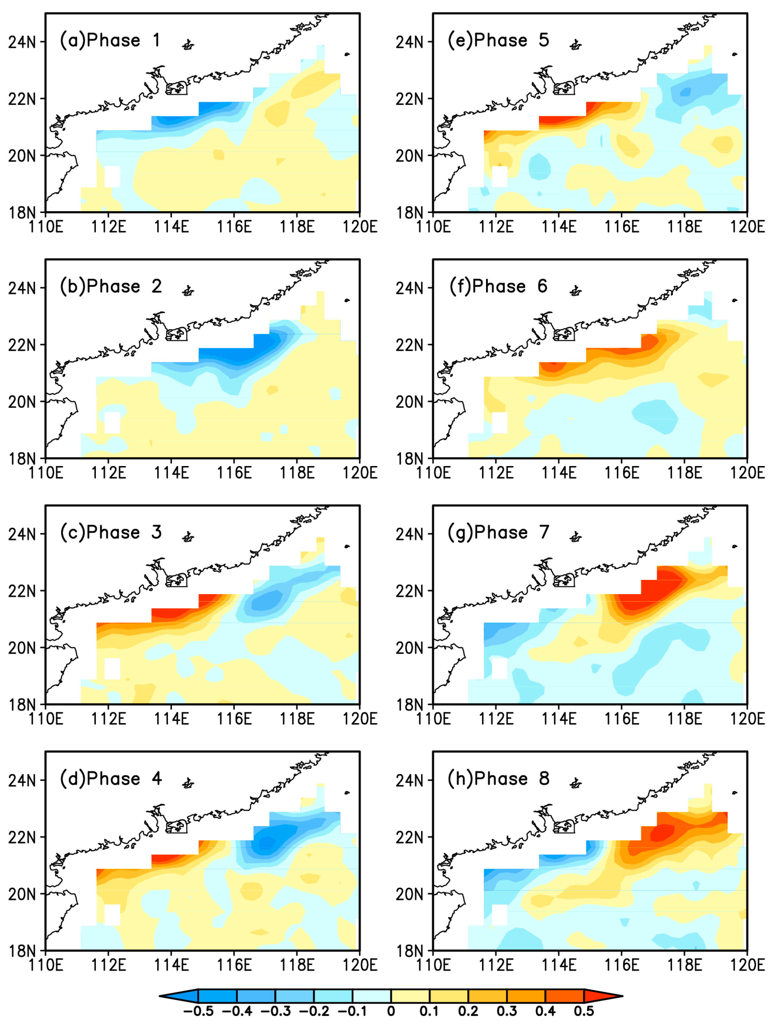
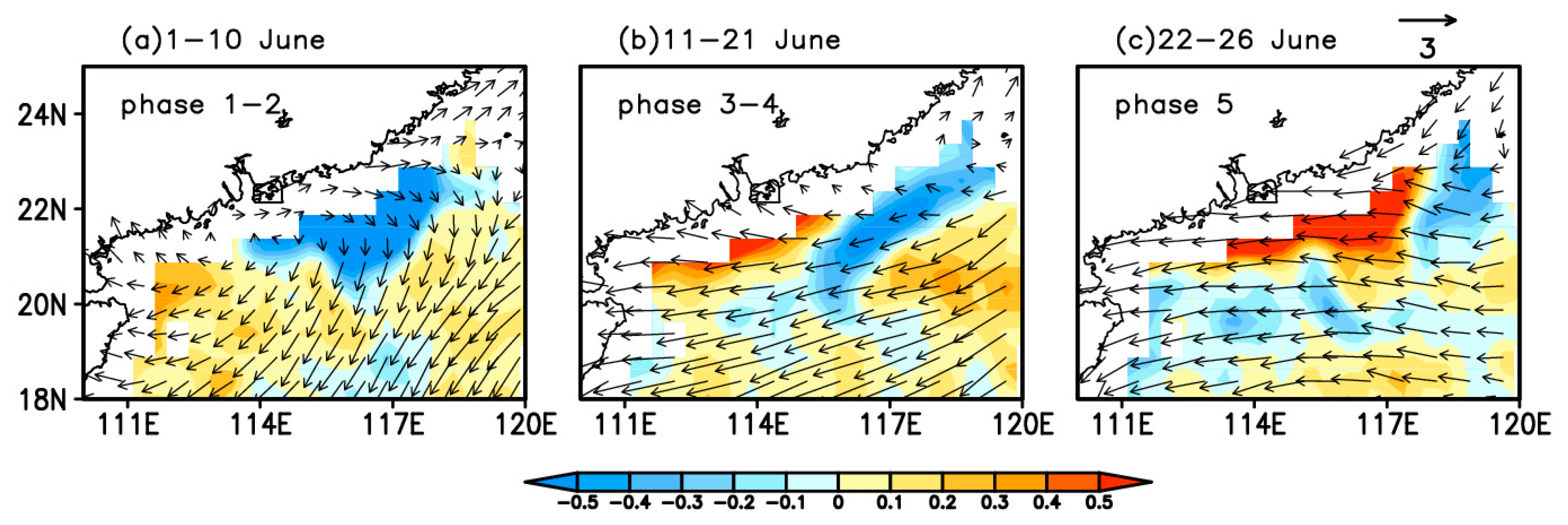
3.2. Madden–Julian Oscillation-Related Offshore Transport of the Plume
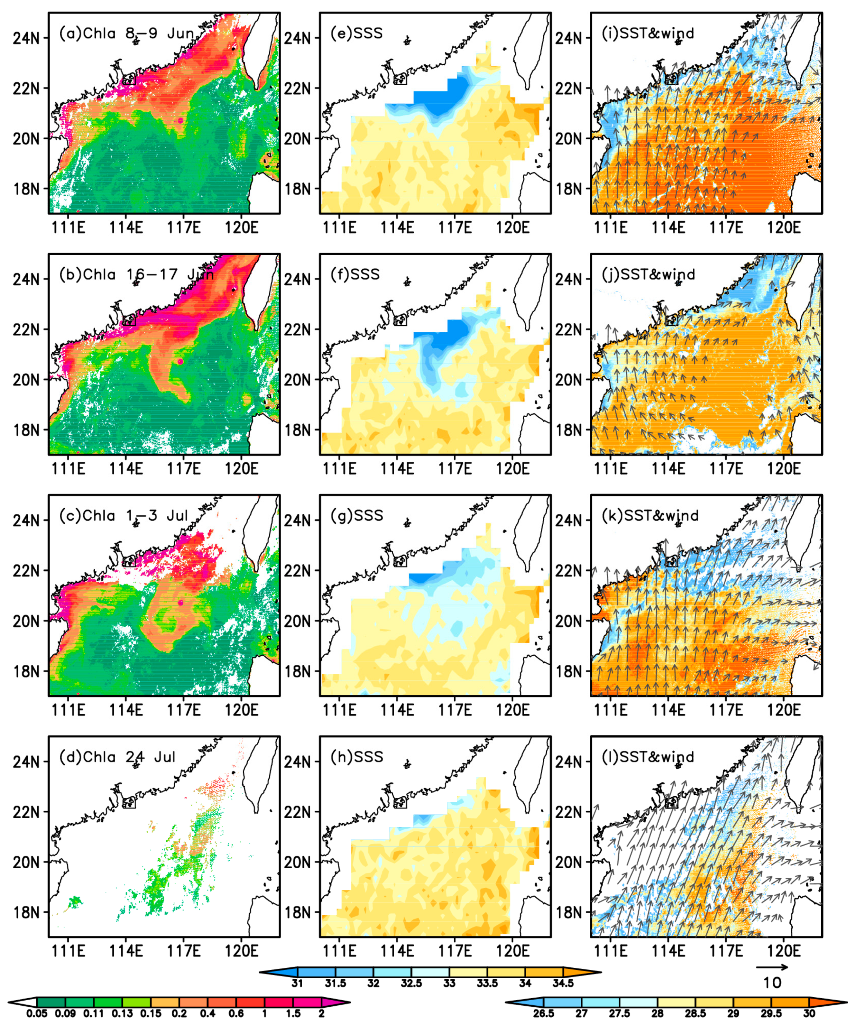
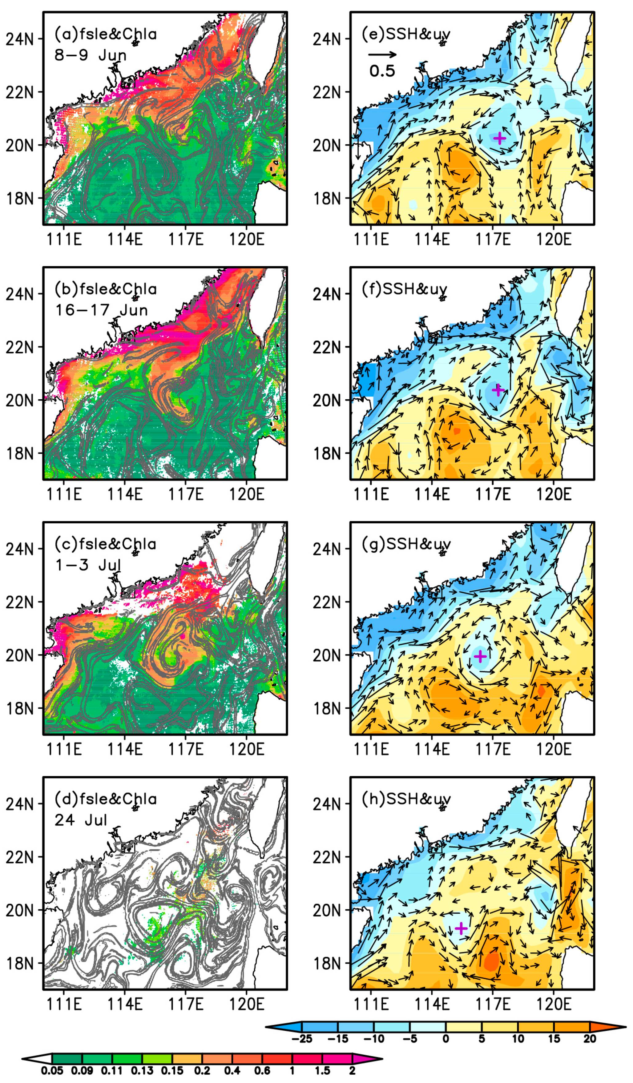
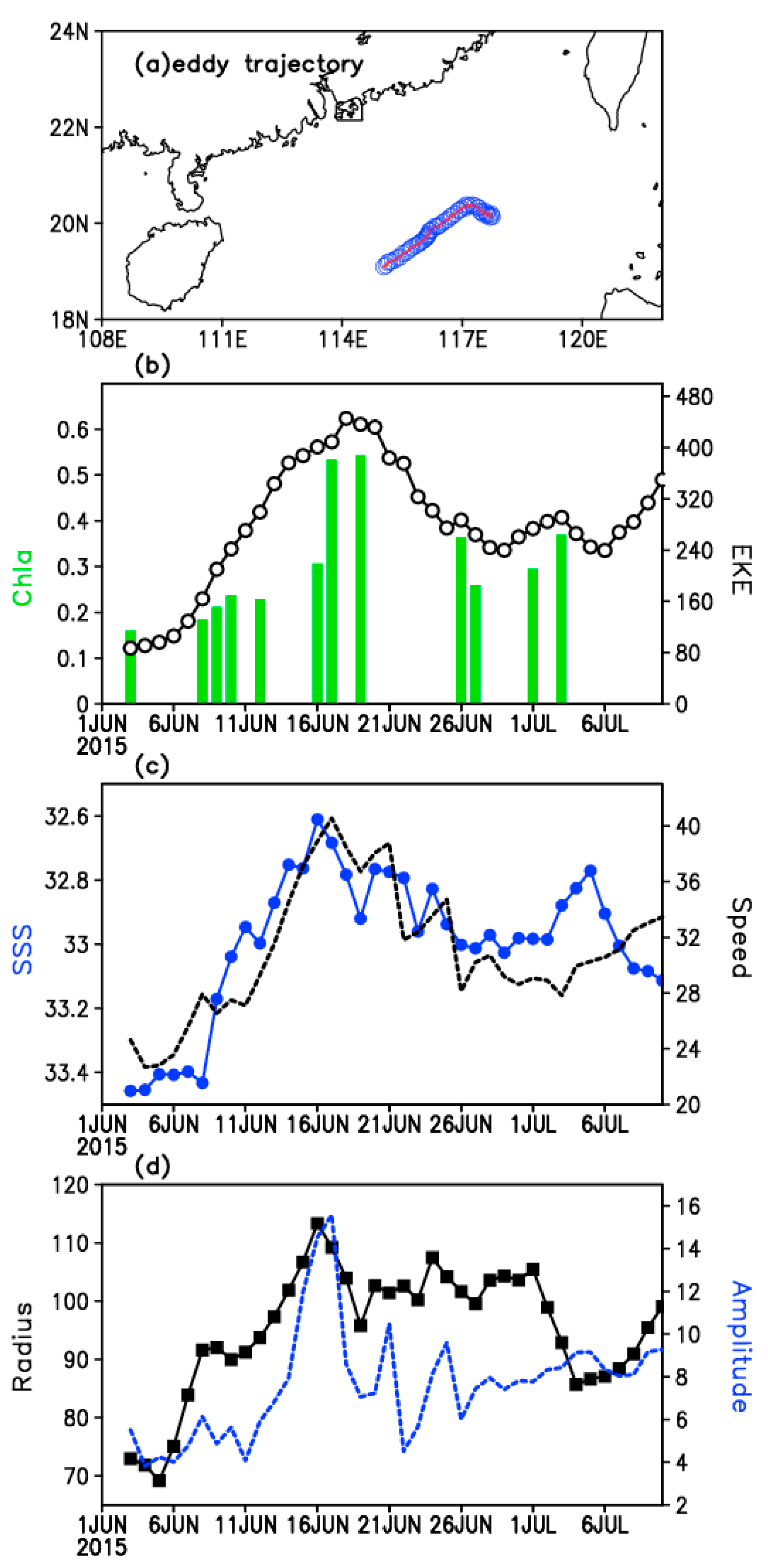
3.3. Impact of Mesoscale Eddies
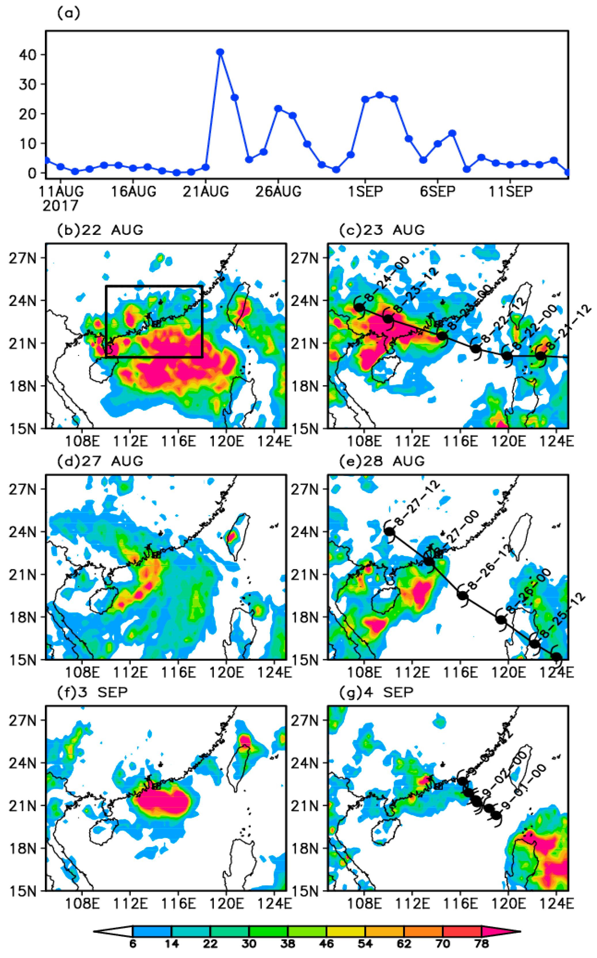
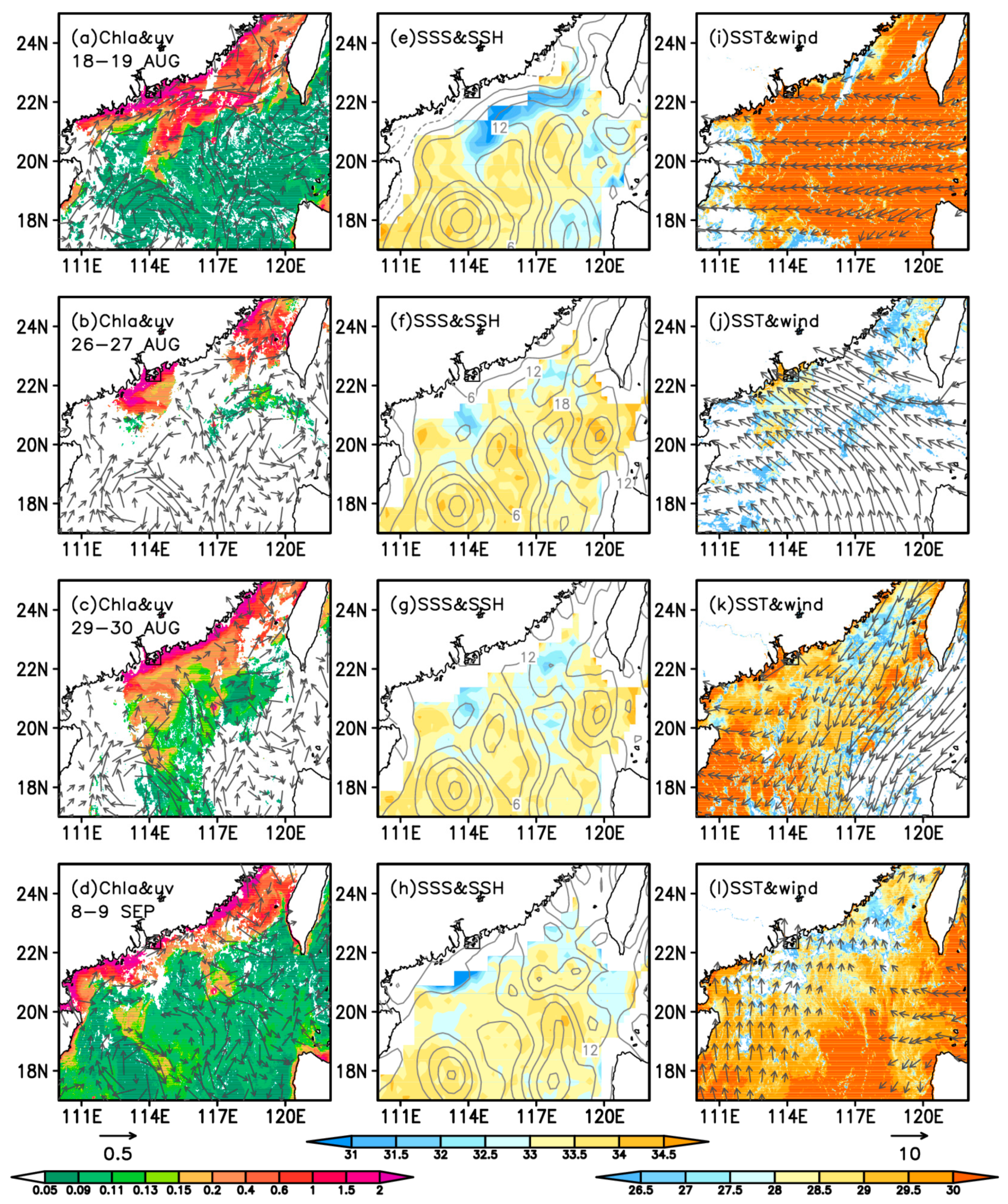
3.4. Role of Tropical Cyclones
4. Summary
Author Contributions
Funding
Acknowledgments
Conflicts of Interest
References
- Hickey, B.M.; Kudela, R.M.; Nash, J.D.; Bruland, K.W.; Peterson, W.T.; MacCready, P.; Lessard, E.J.; Jay, D.A.; Banas, N.S.; Baptista, A.M.; et al. River Influences on Shelf Ecosystems: Introduction and synthesis. J. Geophys. Res. Oceans 2010, 115. [Google Scholar] [CrossRef]
- Gan, J.; Lu, Z.; Dai, M.; Cheung, A.Y.Y.; Liu, H.; Harrison, P. Biological response to intensified upwelling and to a river plume in the northeastern South China Sea: A modeling study. J. Geophys. Res. Oceans 2010, 115. [Google Scholar] [CrossRef]
- Gan, J.; Lu, Z.; Cheung, A.; Dai, M.; Liang, L.; Harrison, P.J.; Zhao, X. Assessing ecosystem response to phosphorus and nitrogen limitation in the Pearl River plume using the Regional Ocean Modeling System (ROMS). J. Geophys. Res. Oceans 2014, 119, 8858–8877. [Google Scholar] [CrossRef]
- Wong, L.A.; Chen, J.; Xue, H.; Dong, L.X.; Su, J.L.; Heinke, G. A model study of the circulation in the Pearl River Estuary (PRE) and its adjacent coastal waters: 1. Simulations and comparison with observations. J. Geophys. Res. Oceans 2003, 108. [Google Scholar] [CrossRef]
- Pan, J.; Gu, Y.; Wang, D. Observations and numerical modeling of the Pearl River plume in summer season. J. Geophys. Res. Oceans 2014, 119, 2480–2500. [Google Scholar] [CrossRef]
- Xie, S.P.; Xie, Q.; Wang, D.X.; Liu, W.T. Summer upwelling in the South China Sea and its role in regional climate variations. J. Geophys. Res. Oceans 2003, 108. [Google Scholar] [CrossRef] [Green Version]
- Chen, Z.; Pan, J.; Jiang, Y. Role of pulsed winds on detachment of low salinity water from the Pearl River Plume: Upwelling and mixing processes. J. Geophys. Res. Oceans 2016, 121, 2769–2788. [Google Scholar] [CrossRef] [Green Version]
- Zu, T.; Gan, J. A numerical study of coupled estuary-shelf circulation around the Pearl River Estuary during summer: Responses to variable winds, tides and river discharge. Deep Sea Res. Part II Top. Stud. Oceanogr. 2015, 117, 53–64. [Google Scholar] [CrossRef]
- Schiller, R.V.; Kourafalou, V.H.; Hogan, P.; Walker, N.D. The dynamics of the Mississippi River plume: Impact of topography, wind and offshore forcing on the fate of plume waters. J. Geophys. Res. Oceans 2011, 116. [Google Scholar] [CrossRef]
- Choi, B.-J.; Wilkin, J.L. The effect of wind on the dispersal of the Hudson River plume. J. Phys. Oceanogr. 2007, 37, 1878–1897. [Google Scholar] [CrossRef]
- Ou, S.; Zhang, H.; Wang, D.-X. Dynamics of the buoyant plume off the Pearl River Estuary in summer. Environ. Fluid Mech. 2009, 9, 471–492. [Google Scholar] [CrossRef] [Green Version]
- Zu, T.; Wang, D.; Gan, J.; Guan, W. On the role of wind and tide in generating variability of Pearl River plume during summer in a coupled wide estuary and shelf system. J. Mar. Syst. 2014, 136, 65–79. [Google Scholar] [CrossRef]
- Jing, Z.; Qi, Y.; Du, Y. Upwelling in the continental shelf of northern South China Sea associated with 1997–1998 El Nino. J. Geophys. Res. Oceans 2011, 116. [Google Scholar] [CrossRef]
- Gan, J.; Li, L.; Wang, D.; Guo, X. Interaction of a river plume with coastal upwelling in the northeastern South China Sea. Cont. Shelf Res. 2009, 29, 728–740. [Google Scholar] [CrossRef]
- He, X.; Xu, D.; Bai, Y.; Pan, D.; Chen, C.-T.A.; Chen, X.; Gong, F. Eddy-entrained Pearl River plume into the oligotrophic basin of the South China Sea. Cont. Shelf Res. 2016, 124, 117–124. [Google Scholar] [CrossRef]
- Shu, Y.; Wang, D.; Zhu, J.; Peng, S. The 4-D structure of upwelling and Pearl River plume in the northern South China Sea during summer 2008 revealed by a data assimilation model. Ocean Model. 2011, 36, 228–241. [Google Scholar] [CrossRef]
- Fong, D.A.; Geyer, W.R. Response of a river plume during an upwelling favorable wind event. J. Geophys. Res. Oceans 2001, 106, 1067–1084. [Google Scholar] [CrossRef]
- Ning, X.; Chai, F.; Xue, H.; Cai, Y.; Liu, C.; Shi, J. Physical-biological oceanographic coupling influencing phytoplankton and primary production in the South China Sea. J. Geophys. Res. Oceans 2004, 109. [Google Scholar] [CrossRef] [Green Version]
- Lu, Z.; Gan, J.; Dai, M.; Cheung, A.Y.Y. The influence of coastal upwelling and a river plume on the subsurface chlorophyll maximum over the shelf of the northeastern South China Sea. J. Mar. Syst. 2010, 82, 35–46. [Google Scholar] [CrossRef]
- Lin, I.; Liu, W.T.; Wu, C.C.; Wong, G.T.F.; Hu, C.M.; Chen, Z.Q.; Liang, W.D.; Yang, Y.; Liu, K.K. New evidence for enhanced ocean primary production triggered by tropical cyclone. Geophys. Res. Lett. 2003, 30. [Google Scholar] [CrossRef] [Green Version]
- Zhao, H.; Tang, D.; Wang, D. Phytoplankton blooms near the Pearl River Estuary induced by Typhoon Nuri. J. Geophys. Res. Oceans 2009, 114. [Google Scholar] [CrossRef]
- Zhang, C.D. Madden-Julian oscillation. Rev. Geophys. 2005, 43. [Google Scholar] [CrossRef] [Green Version]
- Xie, S.-P.; Chang, C.-H.; Xie, Q.; Wang, D. Intraseasonal variability in the summer South China Sea: Wind jet, cold filament, and recirculations. J. Geophys. Res. Oceans 2007, 112. [Google Scholar] [CrossRef]
- Wang, G.; Ling, Z.; Wu, R.; Chen, C. Impacts of the Madden-Julian Oscillation on the Summer South China Sea Ocean Circulation and Temperature. J. Clim. 2013, 26, 8084–8096. [Google Scholar] [CrossRef]
- Ling, Z.; Wang, Y.; Wang, G. Impact of Intraseasonal Oscillations on the Activity of Tropical Cyclones in Summer over the South China Sea. Part I: Local Tropical Cyclones. J. Clim. 2016, 29, 855–868. [Google Scholar] [CrossRef]
- Isoguchi, O.; Kawamura, H. MJO-related summer cooling and phytoplankton blooms in the South China Sea in recent years. Geophys. Res. Lett. 2006, 33. [Google Scholar] [CrossRef]
- Liu, X.; Wang, J.; Cheng, X.; Du, Y. Abnormal upwelling and chlorophyll-a concentration off South Vietnam in summer 2007. J. Geophys. Res. Oceans 2012, 117. [Google Scholar] [CrossRef] [Green Version]
- Chen, Z.; Jiang, Y.; Liu, J.T.; Gong, W. Development of upwelling on pathway and freshwater transport of Pearl River plume in northeastern South China Sea. J. Geophys. Res. Oceans 2017, 122, 6090–6109. [Google Scholar] [CrossRef]
- Vinogradova, N.; Lee, T.; Boutin, J.; Drushka, K.; Fournier, S.; Sabia, R.; Stammer, D.; Bayler, E.; Reul, N.; Gordon, A.; et al. Satellite Salinity Observing System: Recent Discoveries and the Way Forward. Front. Mar. Sci. 2019, 6. [Google Scholar] [CrossRef]
- Guan, B.; Lee, T.; Halkides, D.J.; Waliser, D.E. Aquarius surface salinity and the Madden-Julian Oscillation: The role of salinity in surface layer density and potential energy. Geophys. Res. Lett. 2014, 41, 2858–2869. [Google Scholar] [CrossRef]
- Fournier, S.; Reager, J.T.; Lee, T.; Vazquez-Cuervo, J.; David, C.H.; Gierach, M.M. SMAP observes flooding from land to sea: The Texas event of 2015. Geophys. Res. Lett. 2016, 43, 10338–10346. [Google Scholar] [CrossRef]
- Rahman, M.S.; Di, L.; Yu, E.; Lin, L.; Zhang, C.; Tang, J. Rapid Flood Progress Monitoring in Cropland with NASA SMAP. Remote Sens. 2019, 11, 191. [Google Scholar] [CrossRef] [Green Version]
- Tang, W.; Fore, A.; Yueh, S.; Lee, T.; Hayashi, A.; Sanchez-Franks, A.; Martinez, J.; King, B.; Baranowski, D. Validating SMAP SSS with in situ measurements. Remote Sens. Environ. 2017, 200, 326–340. [Google Scholar] [CrossRef] [Green Version]
- Subrahmanyam, B.; Trott, C.B.; Murty, V.S.N. Detection of Intraseasonal Oscillations in SMAP Salinity in the Bay of Bengal. Geophys. Res. Lett. 2018, 45, 7057–7065. [Google Scholar] [CrossRef]
- Meissner, T.; Wentz, F.J.; Manaster, A.; Lindsley, R. Remote Sensing Systems SMAP Ocean Surface Salinities [Level 2C, Level 3 Running 8-Day, Level 3 Monthly], Version 4.0 Validated release; Remote Sensing Systems: Santa Rosa, CA, USA, 2019. [Google Scholar] [CrossRef]
- Fore, A.G.; Yueh, S.H.; Tang, W.; Stiles, B.W.; Hayashi, A.K. Combined Active/Passive Retrievals of Ocean Vector Wind and Sea Surface Salinity With SMAP. IEEE Trans. Geosci. Remote Sens. 2016, 54, 7396–7404. [Google Scholar] [CrossRef]
- Bentamy, A.; Fillon, D.C. Gridded surface wind fields from Metop/ASCAT measurements. Int. J. Remote Sens. 2012, 33, 1729–1754. [Google Scholar] [CrossRef] [Green Version]
- Mason, E.; Pascual, A.; McWilliams, J.C. A New Sea Surface Height-Based Code for Oceanic Mesoscale Eddy Tracking. J. Atmos. Oceans Technol. 2014, 31, 1181–1188. [Google Scholar] [CrossRef] [Green Version]
- d’Ovidio, F.; Fernandez, V.; Hernandez-Garcia, E.; Lopez, C. Mixing structures in the Mediterranean Sea from finite-size Lyapunov exponents. Geophys. Res. Lett. 2004, 31. [Google Scholar] [CrossRef] [Green Version]
- Wheeler, M.C.; Hendon, H.H. An all-season real-time multivariate MJO index: Development of an index for monitoring and prediction. Mon. Weather Rev. 2004, 132, 1917–1932. [Google Scholar] [CrossRef]
- Lu, X.X. Vulnerability of water discharge of large Chinese rivers to environmental changes: An overview. Reg. Environ. Chang. 2004, 4, 182–191. [Google Scholar] [CrossRef]
- Tian, Q.; Prange, M.; Merkel, U. Precipitation and temperature changes in the major Chinese river basins during 1957–2013 and links to sea surface temperature. J. Hydrol. 2016, 536, 208–221. [Google Scholar] [CrossRef]
- Wu, C.S.; Yang, S.L.; Lei, Y.-P. Quantifying the anthropogenic and climatic impacts on water discharge and sediment load in the Pearl River (Zhujiang), China (1954–2009). J. Hydrol. 2012, 452, 190–204. [Google Scholar] [CrossRef] [Green Version]
- Elsner, J.B.; Liu, K.B. Examining the ENSO-typhoon hypothesis. Clim. Res. 2003, 25, 43–54. [Google Scholar] [CrossRef]
- Liu, K.S.; Chan, J.C.L. Climatological characteristics and seasonal forecasting of tropical cyclones making landfall along the South China coast. Mon. Weather Rev. 2003, 131, 1650–1662. [Google Scholar] [CrossRef]
- Lin, Y.C.; Oey, L.Y. Rainfall-enhanced blooming in typhoon wakes. Sci. Rep. 2016, 6. [Google Scholar] [CrossRef] [PubMed] [Green Version]


© 2020 by the authors. Licensee MDPI, Basel, Switzerland. This article is an open access article distributed under the terms and conditions of the Creative Commons Attribution (CC BY) license (http://creativecommons.org/licenses/by/4.0/).
Share and Cite
Liao, X.; Du, Y.; Wang, T.; Hu, S.; Zhan, H.; Liu, H.; Wu, G. High-Frequency Variations in Pearl River Plume Observed by Soil Moisture Active Passive Sea Surface Salinity. Remote Sens. 2020, 12, 563. https://doi.org/10.3390/rs12030563
Liao X, Du Y, Wang T, Hu S, Zhan H, Liu H, Wu G. High-Frequency Variations in Pearl River Plume Observed by Soil Moisture Active Passive Sea Surface Salinity. Remote Sensing. 2020; 12(3):563. https://doi.org/10.3390/rs12030563
Chicago/Turabian StyleLiao, Xiaomei, Yan Du, Tianyu Wang, Shuibo Hu, Haigang Zhan, Huizeng Liu, and Guofeng Wu. 2020. "High-Frequency Variations in Pearl River Plume Observed by Soil Moisture Active Passive Sea Surface Salinity" Remote Sensing 12, no. 3: 563. https://doi.org/10.3390/rs12030563