Article

Validation of Improved Significant Wave Heights from the Brown-Peaky (BP) Retracker along the East Coast of Australia

School of Engineering, The University of Newcastle, Callaghan NSW 2308, Australia
*
Author to whom correspondence should be addressed.
Remote Sens. 2018, 10(7), 1072; https://doi.org/10.3390/rs10071072
Submission received: 21 May 2018 / Revised: 28 June 2018 / Accepted: 4 July 2018 / Published: 5 July 2018
(This article belongs to the Special Issue Radar Remote Sensing of Oceans and Coastal Areas)

Abstract

:
Improved significant wave heights (SWHs) along the east coast of Australia have been estimated using the parameters resolved by a Brown-peaky (BP) retracker through reprocessing of three years of Jason-1 altimetric waveforms. The BP-estimated SWHs are validated against eight waverider buoys along the coast, and compared with the SWHs estimated by the standard four-parameter maximum likelihood estimator (MLE4). When assessing 1 Hz coastal SWHs for distances from 12 km to the coast, mean standard deviations (STDs) of BP SWHs vary from ca. 0.5 m to 0.9 m, while those of MLE4 SWHs increase from ca. 0.6 m to ca. 2.3 m, indicating a dramatically drop in the quality of MLE4-derived SWHs at the coast. The BP retracker has retrieved ca. 80% of 1 Hz coastal SWHs, which are more than those (ca. 50%) by the standard MLE4. The validation of 1 Hz SWHs is performed by calculating the along-altimeter-track pointwise bias, STD and correlation coefficient between altimetry and buoys. The results show that within 30 km off the coast the BP dataset has better agreement with buoy’s wave heights than the SGDR MLE4 dataset in terms of the BP’s small absolute biases and STDs, as well as high correlation coefficients.

Graphical Abstract

1. Introduction

Accurate significant wave height (SWH) measurements are required in a range of scientific and engineering applications, such as the investigation of wave climate, validation and calibration of wave models, design of offshore engineering structures, and ship routing [1,2,3]. Traditionally, in situ SWH observations are obtained by waverider buoys and voluntary observing ships (VOS) because of their ability to provide high quality measurements with high temporal resolution [4]. The waverider buoy is a floating stainless-steel instrument designed to measure the simultaneous wave height and wave direction. It is often used for calibration and validation of other sensors, but hardly provides suitable datasets for even a basin-scale study due to its sporadic coverage [5]. The VOS data are also limited to the constant commercial ship routes in order to avoid extreme wave conditions for the sake of economic interests [4,5].
Since the launch of the Geosat satellite in 1985, radar altimeters onboard satellites open a new era of monitoring wave heights globally. The conventional radar altimeter emits a pulse towards the sea surface. After interacting with the sea surface, the radar signal reflects off the sea surface and is received by the on-board altimeter. To derive the SWH and other parameters of interest, the shape and magnitude of the recorded power of the signal, called the waveform, are downlinked to the ground post-processing centre and reprocessed by a technique named “waveform retracking”. The principle is to fit the waveform with a physical or empirical model and then solve for unknown parameters [6]. Previous studies have shown that the accuracy of altimeter SWH measurements is similar to that derived from buoys over open oceans [7,8,9]. However, when the satellite approaches the coastal region, the altimeter footprint covers inhomogeneous surfaces (i.e., land topography and calm water), causing contaminated waveforms and thus inaccurate SWHs from the standard retracking procedure.
To overcome the problem, numerous state-of-the-art retracking algorithms have been developed to improve altimeter SWHs at the coast. The performance of retrackers has been validated through comparisons of retracked altimeter SWHs with in situ waverider buoy’s wave data [2,5,10]. Among these work, the adaptive leading edge subwaveform retracker (ALES) by Passaro et al. [11], originally designed to retrieve high quality sea surface heights (SSHs) in coastal regions, shows great superiority in estimation of the SWH data [5]. Other coastal projects, such as Coastal Altimetry (COASTALT) and Processing Innovative System Prototype for Coastal and Hydrology Applications (PISTACH), also make contributions to minimize the wave data gaps within 50 km to the coast [2,10].
Our BP retracker has been recently developed to efficiently retrack coastal waveforms [12]. It provides a seamless dataset of SSHs based on a rule-based combination of a three-parameter weighted least squares (WLS3) estimator and the ALES retracker, extending high quality altimeter measurements right to the coast. Both the WLS3 and ALES adopt the same mathematical model to fit the observed waveform but use different retracking techniques. The WLS3 estimator considers the full waveform and improves the quality of the estimates by downsizing weights at the contaminated gates, while the ALES deals with the sub-waveform (i.e., truncated waveform) to avoid the contaminated gates in the waveform trailing edge [11,12]. The retracked SSHs have been validated against sea level observations by tide gauges around Australia. For detailed information about the BP retracker, readers can refer to [12]. In this paper, SWHs are computed using the parameters estimated by the BP retracker. The BP retracker has the ability to provide accurate wave information for coastal applications, which will be demonstrated in this paper through comparison of the BP-estimated SWHs with in situ waverider buoy’s wave heights along the Australian east coast.
In Section 2, the study area and dominant factors affecting the wave conditions over the study area are represented, as well as the buoy and altimetry datasets used for the validation. Section 3 introduces methods of SWH estimation using the BP-resolved parameters and validation of the altimeter SWHs against the buoy wave data. Section 4 evaluates the BP-estimated SWHs by comparing with wave heights obtained by the standard MLE4 retracker and buoys. Section 5 represents and discusses the validation results of SWHs against buoy data along altimetry ground tracks with 1 Hz sampling frequency. Section 6 draws the conclusion of the study.

2. Data and Study Area
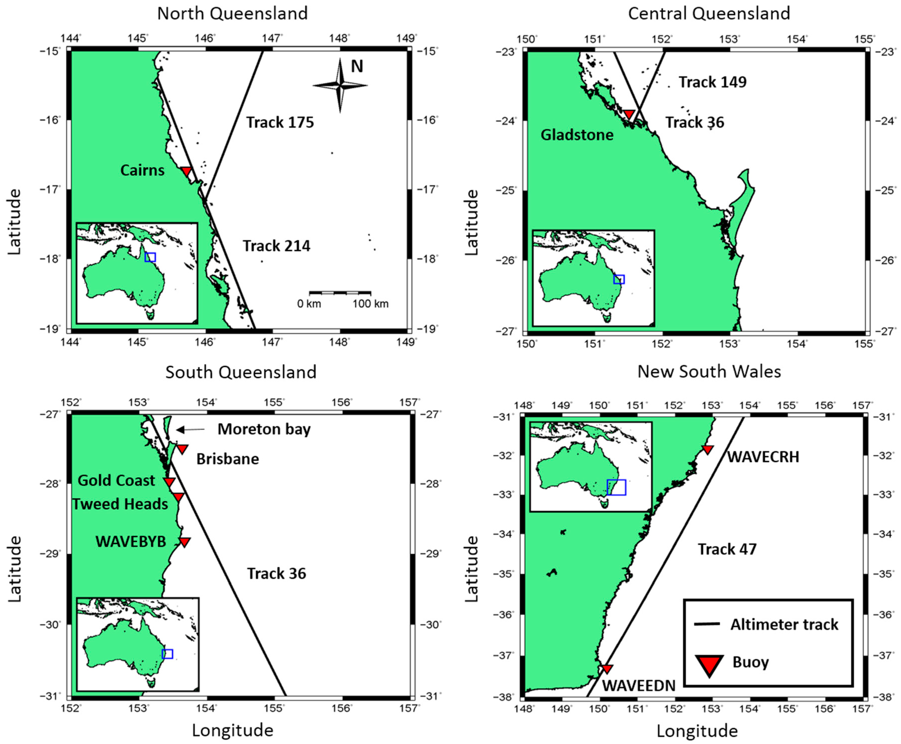
2.1. Study Area

Four areas (Figure 1) along the east coast of Australia (15°S–38°S, 144°E–157°E) are selected to validate the estimated SWHs from the BP retracker against in situ wave heights obtained from offshore waverider buoys. The selection of this region is due to the availability of both buoy and altimeter data at coastal zones. To the north between latitudes 15°S and 25°S in the Great Barrier Reef system, the wind and wave climate is strongly seasonal and affected by the austral summer monsoons [13]. The wave conditions of the Great Barrier Reef depend largely on locally generated wind waves [14]. Moving south along the New South Wales coast, the generally moderate wave climate exhibits an average offshore SWH of 1.5–1.6 m and is periodically affected by large wave events induced by the coastal storm systems [15]. Therefore, the complex coastal morphology and wave climate provide a challenging test region to evaluate the performance of the BP retracker.

2.2. Data

Three years of data between February 2009 and February 2012 are used in this study. They are (1) the in situ wave data from eight waverider buoys; (2) three years of Jason-1 waveforms (cycles 263–372) and (3) SWHs provided by Sensor Geophysical Data Record (SGDR) products. The selected altimetric ground tracks and buoys are located along the east coast of Australia (Figure 1). All buoys are within 13 km from the coastline (Table 1). In Queensland, the SWHs from buoys have a sampling interval of 30 min and were supplied by the Queensland government. Other buoy SWHs in New South Wales have a sampling interval of 1 h and are available from the Australian Ocean Data Network (AODN, https://portal.aodn.org.au/). These buoys are usually deployed in 70–100 m water depth on the mid-continental shelf [15].
Within the study region, there are three ascending tracks (47, 149, and 175) and two descending tracks (36 and 214) from Jason-1 (Figure 1). Tracks 36, 47, and 214 are parallel to the coastline, while tracks 149 and 175 move in a land-to-sea transition. Note that the flight direction of the satellite towards the coastline impacts the behaviour of the onboard tracker. The tracker takes more time (ca. 1 s) to keep the received signals within the radar observation window for the land-to-sea transition [2,5].
The SWH is defined as the average of one-third of the highest wave heights and is usually quantified as four times the STD of wave heights [5]. The waverider buoy’s SWH is derived from the measured wave heights, while the altimeter’s SWH is individually estimated from an analysis of the return waveform. The widely used altimeter SWH data are the 1 Hz along-track SWHs (corresponding to a distance ca. 7 km). The buoy measurement is the average of a given point over a period of time (20–30 min), while the radar altimeter observation is the average of the footprint with the diameter being 2–20 km for Jason-1 at a given instant of time. Therefore, these two sources of SWHs are comparable, but there still exists discrepancies in their SWH measurements due to the temporal and spatial proximity and different sampling manners [16,17].
According to the recommendations from previous studies [8,16,17,18,19,20], we will only use Jason-1 along-track data within 50 km from the corresponding buoy. Table 1 lists information about the buoy, the ground tracks, distance between the buoy and track, and distance between the buoy and the coast.

3. Methods

3.1. Estimation of SWH

The SWH can be computed using the parameters estimated by the retracker [5,7]. The BP retracker solves three unknown parameters [12]. They are: (1) the waveform amplitude Pu, which is associated with the backscatter coefficient and ocean surface wind speed; (2) the epoch τ, which is related to the position of the midpoint of the leading edge with respect to the pre-designed tracking gate; and (3) the slope of rise time of the leading edge σc, from which the SWHs can be derived. The parameter σ c can be expressed as [5,21]:
σ c 2 = σ p 2 + σ s 2   and   σ s = SWH 2 c
SWH = 2 c σ c 2 σ p 2
where σp is the standard deviation of Gaussian-modelled point target response (PTR), σs the standard deviation of the ocean height and c the speed of light. For Jason-1, σ p = 0.513 r t is used and r t = 3.125 ns is the time interval between two adjacent waveform gates [6]. The PTR is approximated by a Gaussian function in order to derive the analytical function of the Brown model. Compared to other parameters, σp has the largest influence on the accuracy of the SWH estimates [22]. As such, a dedicated SWH correction is derived from a look-up table and provided in the SGDR product [23,24]. The corrected SWH is then calculated as:
corrected   SWH = estimated   SWH + SWH   correction
to obtain the SWH from the BP retracker, three steps are involved. The first step is to fit the Brown model to the waveform leading edge and solve the preliminary SWH by the unweighted least squares estimator. The second step is to detect the peaky gates contained in the waveform and resolve the SWH parameter using the WLS3 estimator. The final step is to compare the difference between the SWH from the leading edge retracker and the WLS3 estimator. If the difference is <2 m, the SWH from the WLS3 estimator is the output of the BP retracker. This procedure is different from the ALES [11] in that the BP considers full waveforms but estimates parameters based on detected waveform peaks using the WLS3 estimator. A detailed description of the BP retracker can be found in [12].

3.2. Methods for the SWH Evaluation and Validation

The 20 Hz BP-derived SWHs are estimated using the BP retracker based on the methods mentioned in Section 3.1. The estimated 20 Hz SWHs can be used to generate the 1 Hz SWH data, which are commonly used in scientific and engineering applications [5,8]. In this study, a rigorous quality control was first undertaken to delete spurious 20 Hz observations within each 1 Hz block, i.e., points with SWH values larger than 8 m were removed, as well as observations outside the 95% confidence interval. The 1 Hz SWH data were then calculated as the mean value of remaining observations of each 1 Hz block. For comparison, we also used 1 Hz SWHs officially provided in the SGDR product, which are originally computed using the parameters from the MLE4 retracker [8] (hereafter called the SGDR MLE4 SWHs).
The data quality and availability of SWHs were evaluated by comparing BP-derived SWHs (hereafter called the BP SWHs) with (1) SGDR MLE4 SWHs; and (2) buoy wave heights in Section 4. In addition, the altimeter 1 Hz SWH time series were validated against buoy wave-height measurements in terms of the mean difference (hereafter called the bias), STD and correlation coefficient at each altimeter along-track point in Section 5. Since the reliability of these statistics depends on the number of observations used in computations, the significance of the correlation coefficient was tested using Student’s t-test. We found that the time series of altimeter and buoy SWHs are correlated at the 95% significance level, if the sample size is ≥30 and the correlation coefficient ≥0.4. We also found that the negative correlation unreasonably occurs if the number of observations is less than 30. Therefore, the statistics are calculated only if the number of SWHs in a time series at an along-track point is larger than 30. The validation was conducted as follows:
  • Using Jason-1 nominal tracks provided by the Centre for Topographic studies of the Ocean and Hydrosphere (CTOH, http://ctoh.legos.obs-mip.fr/altimetry/satellites), the altimetric SWHs are linearly interpolated to the corresponding nominal track;
  • The buoy wave heights are interpolated to the same time as the altimeter SWH data;
  • The difference (i.e., bias) between the buoy and 1 Hz altimeter SWHs is calculated at each along-track point for all cycles;
  • The mean and STD of the SWH differences, and correlation coefficient between the altimeter and buoy wave heights are calculated at each along-track point.

4. Evaluation of BP-Estimated SWHs

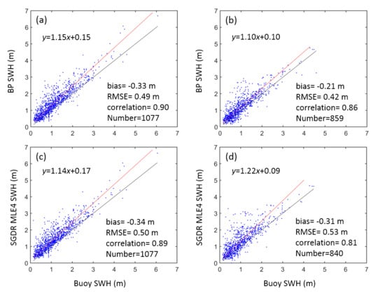
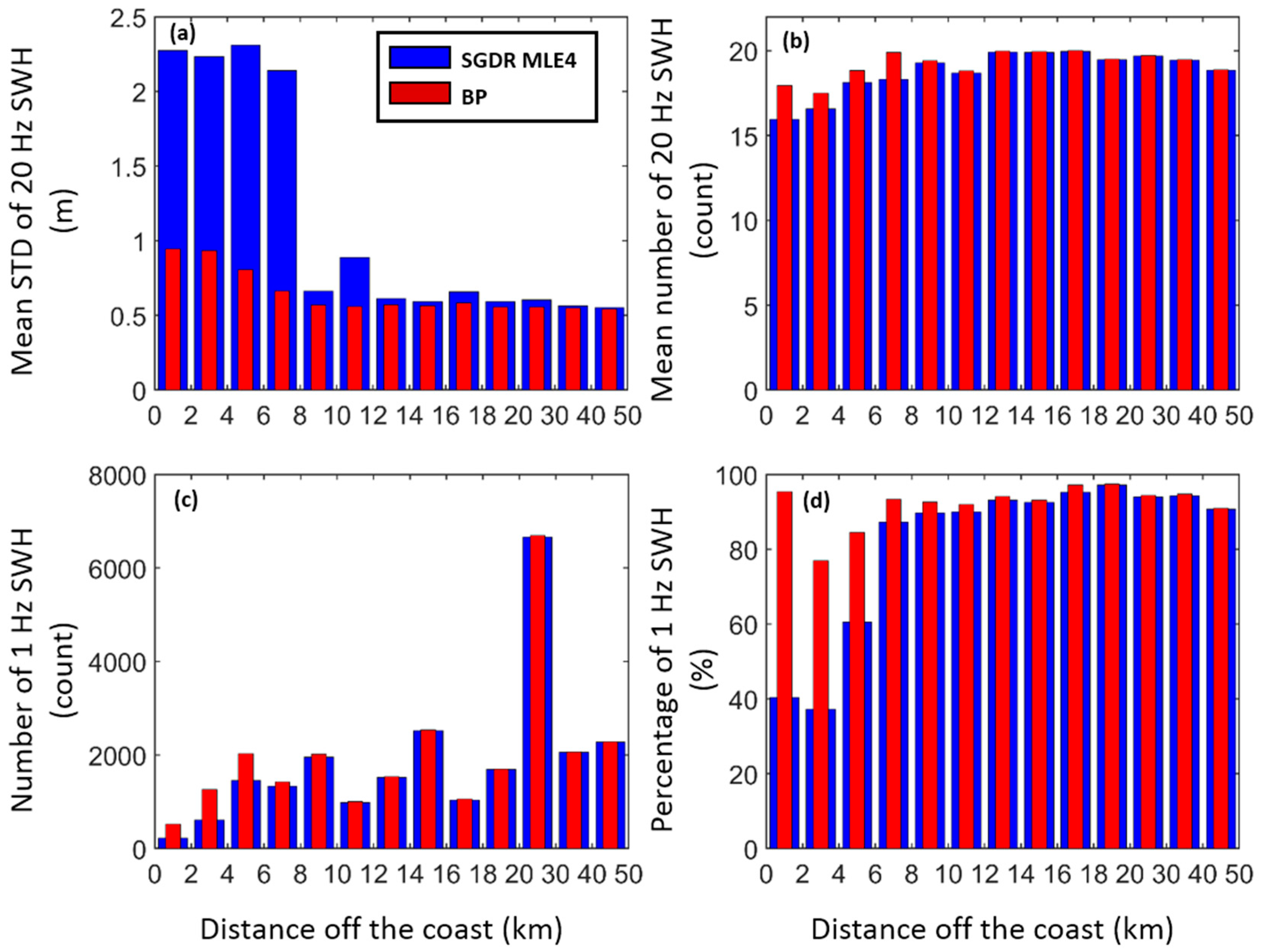
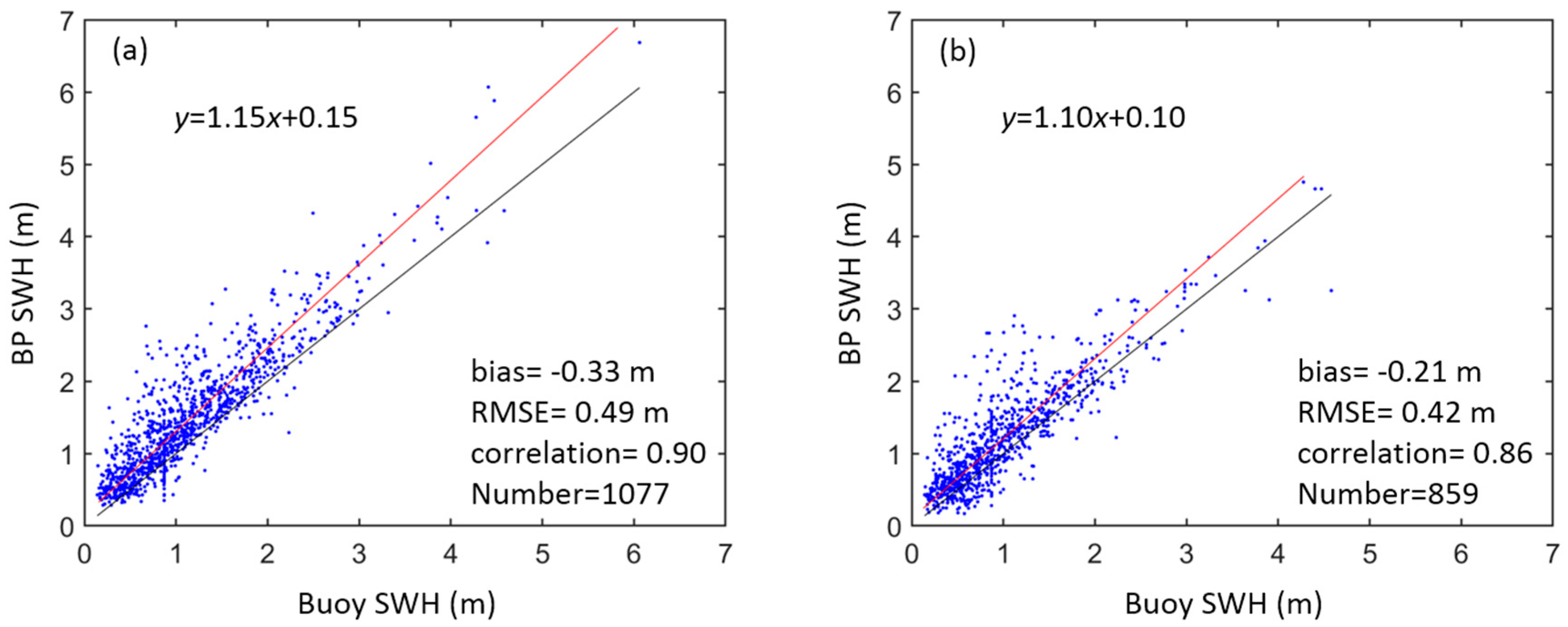
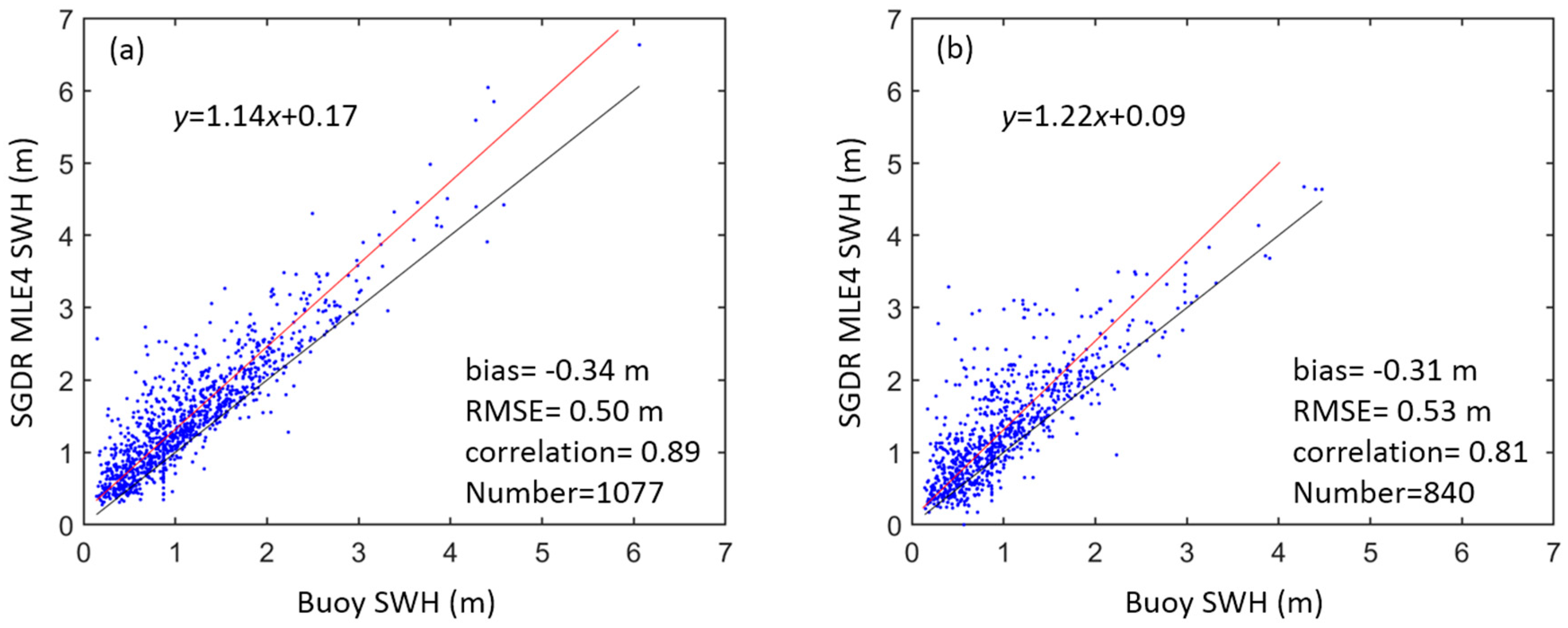
4.1. Comparison between BP and SGDR MLE4 SWHs

The purpose of the evaluation is to assess the data quality and availability based on all retrieved SWHs from BP and SGDR MLE4 retrackers. For each 1 Hz data block, the STD and number of 20 Hz BP SWHs are calculated, while these data for SGDR MLE4 SWHs were directly obtained from the SGDR product. The comparison was conducted within 50 km from the coast. This zone was divided into 13 bands with widths of 2 km at distances 0–20 km from the coast, and widths of 10 km at distances 20–50 km from the coast. For each zone, the mean STD of 20 Hz SWHs (Figure 2a), the mean number of 20 Hz SWHs (Figure 2b), the total number of 1 Hz SWHs (Figure 2c), and the percentage of retrieved 1 Hz SWHs (Figure 2d) were calculated.
As can be seen in Figure 2a, the mean STDs beyond 12 km offshore are ca. 0.55 m for both BP and MLE4 SWH datasets. Between 8 and 12 km from the coast, the mean STDs for SGDR MLE4 start to increase, while BP still retains its mean STDs at the same level (ca. 0.55 m) as those over the open ocean. Within 8 km from the coastline, the mean STDs for SGDR MLE4-estimated SWHs increase sharply from ca. 0.6 m to ca. 2.3m, but the BP STDs only increase slightly from ca. 0.5 m to 0.9 m. This suggests a remarkable improvement of the BP dataset compared to the SGDR MLE4 over nearshore distances (0–8 km). Figure 2b illustrates the mean numbers of 20 Hz SWHs available in different zones. The numbers of the BP are similar to those of the SGDR MLE4 for distance >8 km from the coast, but slightly better than the SGDR MLE4 for distance <8 km to the coast, where the BP has 1–3 more SWHs within the 1 Hz block. When the distance is <2 km to the shore, the SGDR MLE4 has, in average, the smallest mean number (ca. 15) of 20 Hz SWHs, implying the degradation of the data availability.
From beyond 6 km (Figure 2c) off the coast, the total number of retrieved 1 Hz SWHs for BP is similar to that for SGDR MLE4. Within 6 km to the coast, the BP recovers more SWHs than the SGDR MLE4. The similar pattern is also shown in Figure 2d. Both BP and SGDR MLE4 derive more than 90% of 1 Hz SWHs when the distance to the coast is >12 km. Within 12 km to the coast, the BP still retrieves ca. 80% of 1 Hz SWHs, while the percentage of SWHs retrieved by the SGDR MLE4 drops from ca. 85% to 40%.
From the above analysis, we learn that the BP’s improvement in terms of data precision and availability mainly occurs within the distance <12 km to the coast, in particular within 0–8 km, where the mean STDs of the BP are significantly smaller (Figure 2a) and mean numbers of the BP are relatively larger (Figure 2b) than those from the SGDR MLE4. We also find that the BP’s mean STDs within 6 km to the coast are between ca. 0.6 m and 0.9 m, suggesting that the retracked SWH data should be used with caution and that further improvement in the retracker is required for coastal SWH applications.

4.2. Comparison Between BP-Estimated SWHs and Buoy Wave Heights

In this section, the performance of BP is also assessed by the comparison between the averaged BP and buoy SWHs, while the pointwise validation of the 1 Hz BP SWHs against buoy data will be presented in Section 5. From Section 2.2, the altimeter along-track SWHs are considered within 50 km radius of the buoy, while buoys are located near the coast with distance <ca. 13 km. Therefore, the assessment is performed in two coastal zones for distances 0–12 km and 12–50 km to the coast, respectively. For a particular buoy, the buoy and corresponding altimeter SWHs were averaged for each cycle. All averaged buoy and altimeter SWHs from different cycles were used for the comparison. The altimeter-derived SWHs near Brisbane are not used for this analysis due to their poor quality (see Section 5.3). The linear relationship between SWHs from buoys and altimetry was estimated by orthogonal regression analysis (or major axis regression) because both estimates from altimetry and buoys have uncertainties [9,19,20]. The regression considers errors in both SWH datasets and minimizes the sum of squares of orthogonal projections from the SWH to the best-fit line [20,25,26].
Figure 3 and Figure 4 show the scatter plots of all pairs of altimeter and buoy SWHs in the two coastal zones, and the corresponding fitted lines (in red) resulting from the regression analysis. The unity slope (in black) reveals the theoretical consistency between the altimeter and buoy SWHs. The positive interceptions shown in the regression functions indicate that altimeter-derived SWHs are overestimated in the study area, this agrees with [2,5,10]. Most SWHs displayed in Figure 3 and Figure 4 are relatively low (<4 m) due to the sheltering effect of the Australian landmasses [27].
Figure 3a and Figure 4a show that both the BP and the SGDR MLE4 achieve similar results in comparison with the buoy SWHs in the coastal zone 12–50 km, where there are 1077 SWHs from each dataset. The high correlation (ca. 0.90) between altimeter and buoy SWHs indicates that the altimeter is able to capture the seasonal variability of SWHs. The RMSE (ca. 0.5 m) for both BP and SGDR MLE4 is relatively large, but still reasonable due to different sampling manners between altimeter and waverider buoy [16,17]. The estimated negative biases for the BP (−0.33 m) and SGDR MLE4 (−0.34 m) again demonstrate the overestimation of altimeter SWHs. Since the overestimation is also reported when validating of the PISTACH product against buoys [10], we are confident that bias estimates from this study are comparable with those by other researchers in coastal zones [5]. The statistical results suggest that both BP and SGDR MLE4 SWHs have similar accuracy for offshore distances 12–50 km.
Figure 3b and Figure 4b show the comparison of BP and SGDR MLE4 SWHs with buoy data in the coastal zone 0–12 km, where different statistical results between BP and SGDR MLE4 can be seen. The BP retracker is superior to the SGDR MLE4 in case of the smaller RMSE (0.42 m vs. 0.53 m), slightly stronger correlation (0.86 vs. 0.81), and a higher number of retrieved SWHs (859 vs. 840). In this nearshore zone, SWHs range typically from 0–3 m, which is ca. 1 m lower than those within the 12–50 km coastal zone. The magnitude of bias (−0.21 m) for BP is smaller than that (−0.31 m) for SGDR MLE4. The results suggest that BP SWHs are more consistent with the buoy SWHs and, therefore, more accurate than the SGDR MLE4 for monitoring wave heights in the nearshore zone.

5. Validation of 1 Hz Along-Track SWHs

The validation of 1 Hz along-track SWHs against buoy wave heights is performed according to buoy locations in the North Queensland, Central Queensland, South Queensland, and New South Wales (cf. Figure 1). In Section 5.1, Section 5.2, Section 5.3 and Section 5.4, Figure 5, Figure 6, Figure 7, Figure 8 and Figure 9 show the validation results of 1 Hz along-track SWHs (from both BP and MLE4) against buoy wave heights in different areas in terms of point-wise bias, STD of the difference between 1 Hz SWHs and buoy values, and correlation coefficient for Jason-1 tracks used in this study. In Figure 5, Figure 6, Figure 7, Figure 8 and Figure 9, the green line illustrates the distance of the along-track points to the coast. The along-track point that has the shortest distance to the buoy represents the buoy’s location (in black vertical dash line). Some common issues are discussed in Section 5.5.

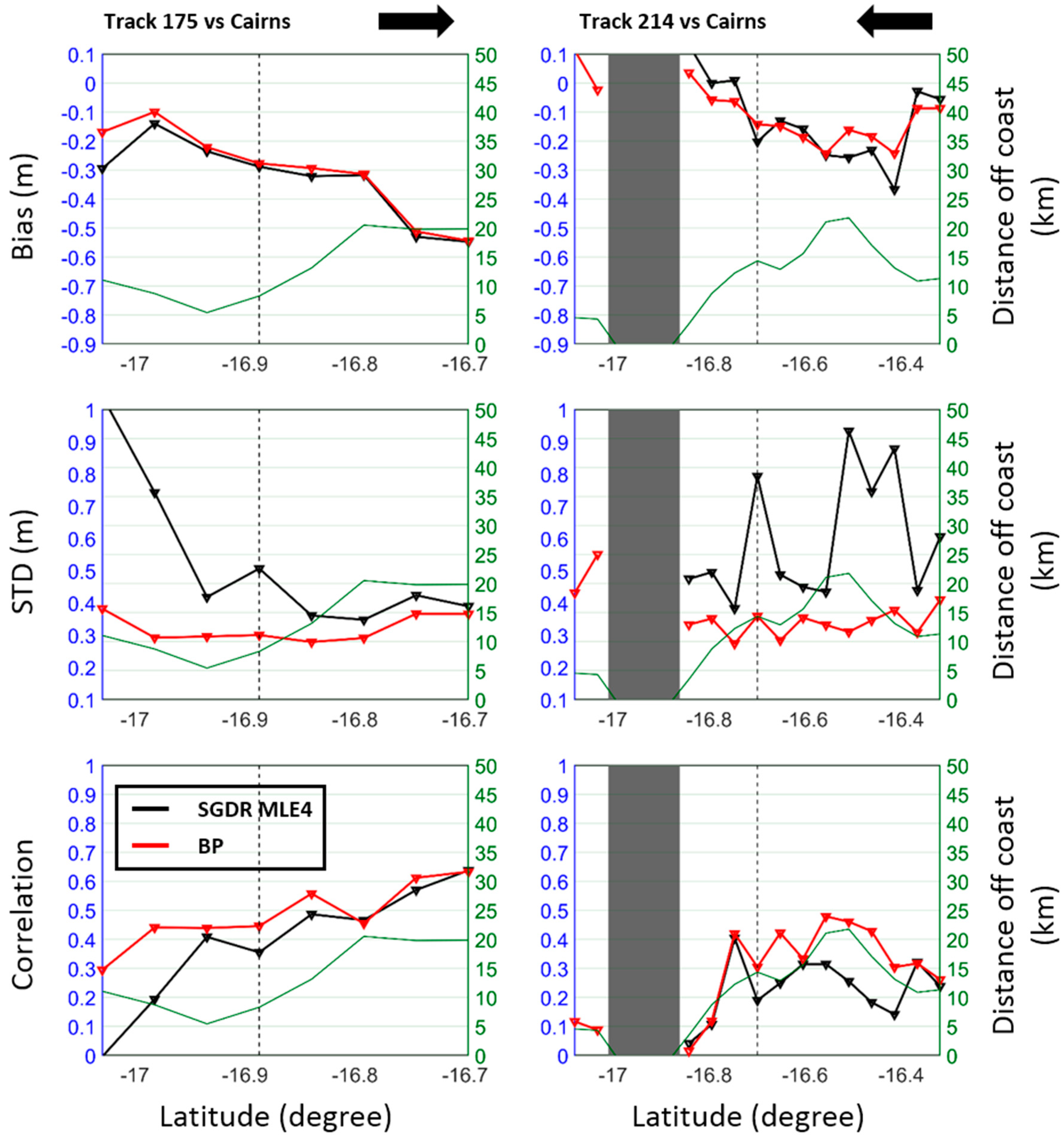
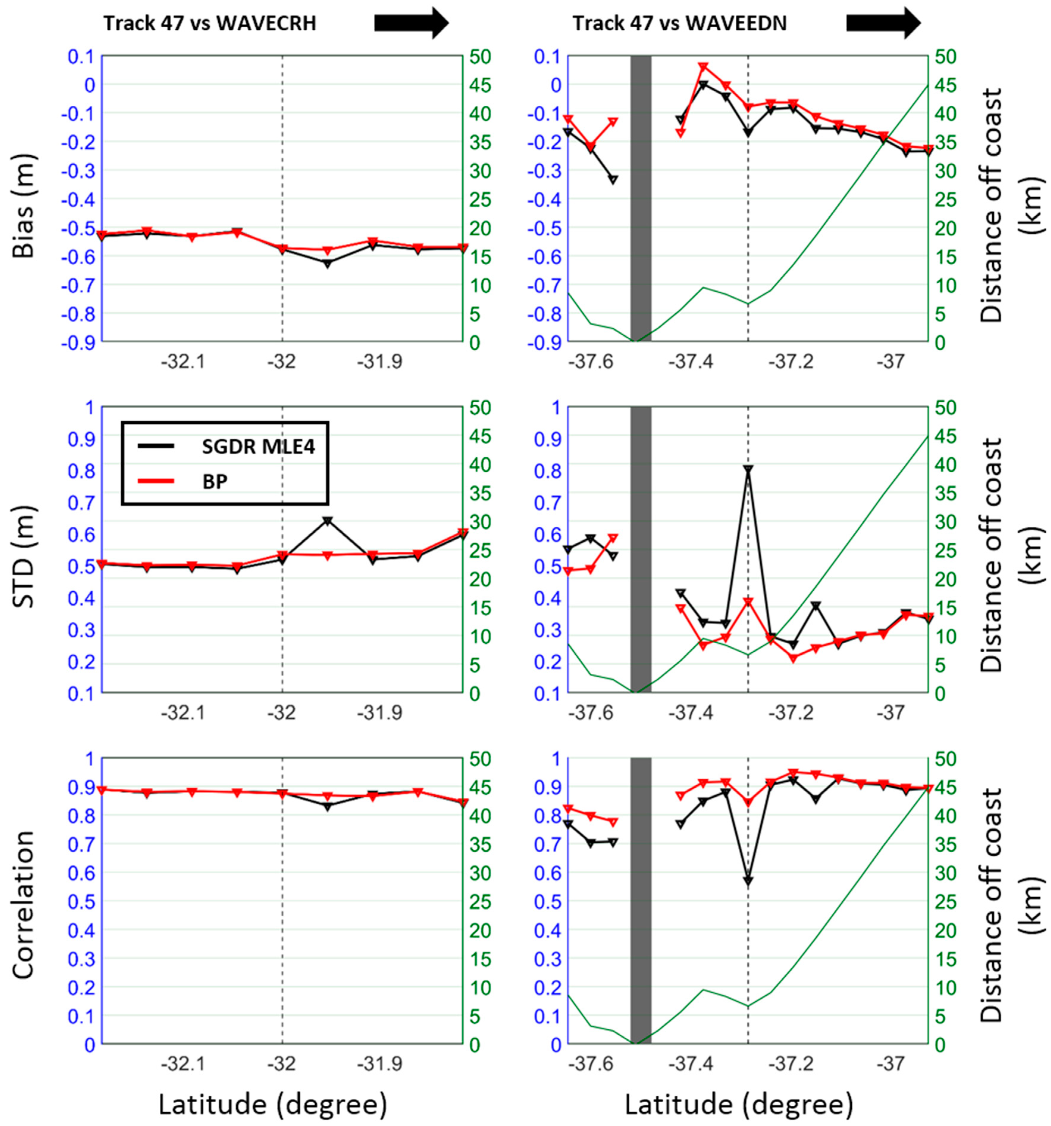
5.1. North Queensland

In this area (Figure 5), the buoy is located on the narrow continental shelf (~16.7°S) separated from the open ocean by the Great Barrier Reef, where the reefs affects the propagation of the waves and attenuates the offshore wave energy [14,28]. The presence of the Australian mainland and surrounding islands results in complicated waveform shapes that cannot be followed by the standard MLE4 retracking algorithm and, therefore, causing large uncertainty in SGDR MLE4 SWHs (cf. mid panel in Figure 5).
Track 175 (left in Figure 5) moves in a land-to-sea transition; all selected points along track 175 are ca. 45–50 km away from the buoy at Cairns (Table 1). It can be seen that bias profiles of both BP and SGDR MLE4 product vary in a similar pattern, but absolute values of biases from the BP retracker are smaller (from ca. 0.10 m to ca. 0.54 m) than those (from ca. 0.16 m to ca. 0.54 m) by the SGDR MLE4. The STDs for BP are constantly below 0.4 m, while STDs for SGDR MLE4 largely fluctuate between 0.3 and 0.75 m. The along-track correlation (0.3–0.6) between SWHs from BP and the buoy are higher than that (0.1–0.6) between SWHs from SGDR MLE4 and the buoy. The statistical results along track 175 suggest that the BP is a superior retracker for processing waveforms over the Great Barrier Reef.
Track 214 (right in Figure 5) is close and parallel to the coastline with the selected along-track points symmetric with respect to the buoy at Cairns (Figure 1). When the altimeter returns are not corrupted by the land reflection, the absolute biases of the BP show a similar behaviour to that of the SGDR MLE4, varying between 0.1 and 0.2 m. The significant change in the SGDR MLE4 results occurs when the track is within a distance <10 km to the coast due mainly to land contamination. In contrast, the BP’s along-track results show smaller STDs (ca. 0.4 m) and higher correlations (0.3–0.5) when compared to SGDR MLE4. However, the relatively low correlation (<0.5) between SWHs from BP and buoy again demonstrates the complex wave climate in this area. Although the minimum bias (ca. 0.0 m) is observed at the point near the coastline, the corresponding correlation coefficient (<0.3) is beyond the 95% significance level. This means that the minimum bias is unreliable. Considering the reliability of all the statistics, the robust bias estimation ranges from −0.1 m to −0.5 m at Cairns in North Queensland.

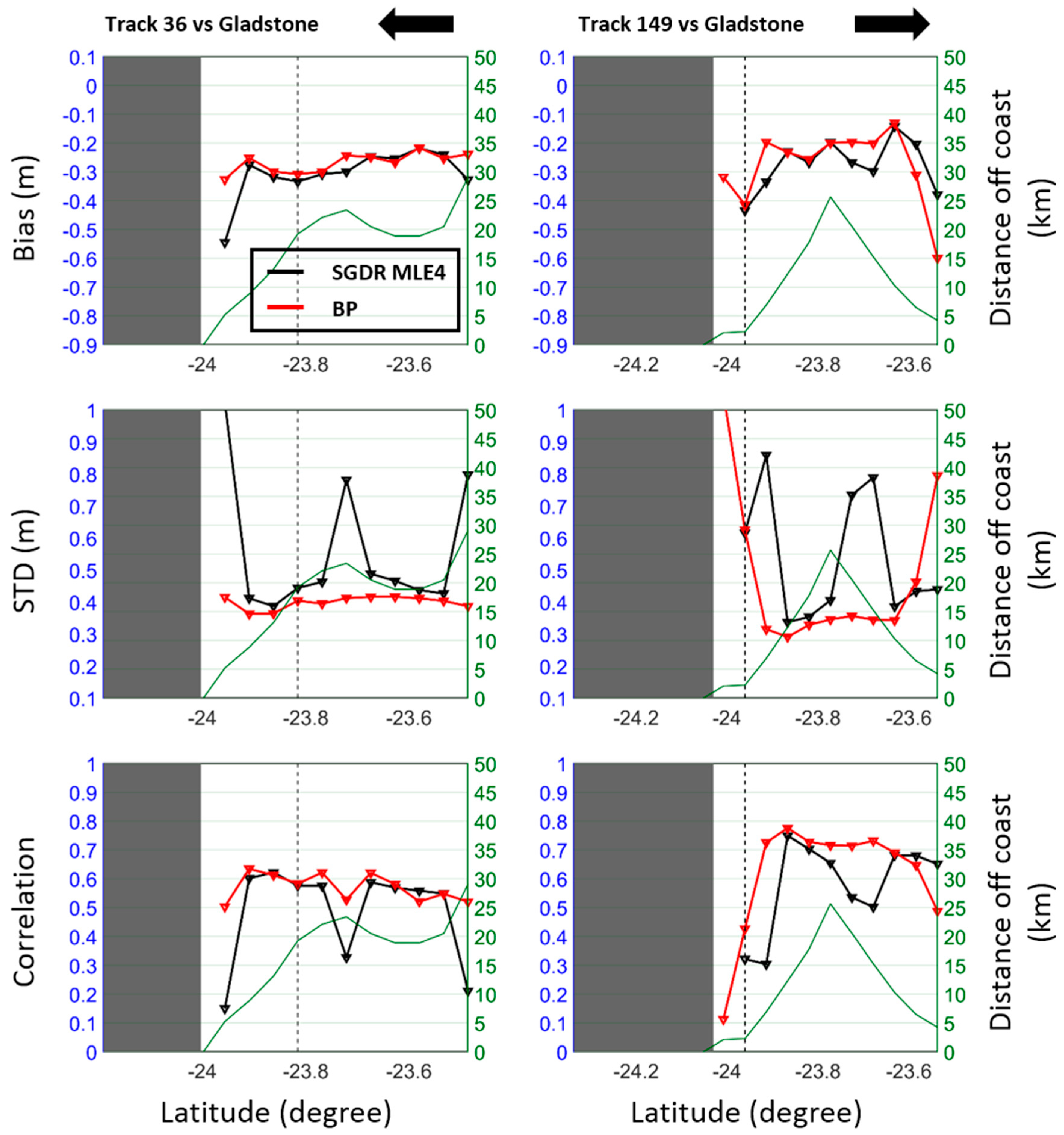
5.2. Central Queensland

In this area (Figure 6), the wider continental shelf provides a large surface area of shallow water, thus the impact of the wind on the local wave climate is strengthened [29]. Both tracks 36 (left in Figure 6) and 149 (right in Figure 6) are over the continental shelf, leading to similar results. Beyond ca. 8 km offshore, the absolute biases are generally around 0.2–0.3 m for both SGDR MLE4 and BP datasets. The improvement of the BP can be seen along entire tracks, except for some nearshore points (<5 km) of track 149. The BP has smooth along-track STDs (ca. 0.4 m) and strong correlations with the buoy (>0.5), while the SGDR MLE4 displays fluctuated STDs and correlations. The results support that the BP SWHs are more precise than SGDR MLE4 SWHs along both tracks around the Gladstone buoy.
When track 149 is very close to the coast (<2 km) in the area south of 23.9°S (right in Figure 6), the data quality of both BP and SGDR MLE4 shows significant deterioration. It is because the observed waveforms are quite noisy and are unlikely to accurately resolve the SWH estimates. The degradation north of 23.75°S is attributed to Masthead Island, which is a coral cay located in the Southern Great Barrier Reef. The relatively worse performance for land-to-sea track 149 compared to sea-to-land track 36 may result from the operation mode of the altimeter related to the satellite flight direction as stated in Section 2.2. The altimeter needs ca. 1 s to relocate the returned echoes within the radar observation window [6], causing a longer land contamination distance in track 149.

5.3. South Queensland

In South Queensland, four selected buoys are distributed from north to south along the coastline at Brisbane, Gold Coast, Tweed Heads, and WAVEBYB (Figure 1). Of them, Gold Coast and Tweed Heads buoys have the shortest distance (<1.6 m) to the coast. They are also relatively close together, which would experience similar nearshore wave climates. The descending track 36 is nearly parallel to the coastline, passing southeastward over the ocean. Validation results of 1 Hz along-track SWHs against buoy wave heights are shown in Figure 7 and Figure 8.
Brisbane buoy (left in Figure 7) is located near the entrance of Moreton Bay, which is separated from the Coral Sea by three sand islands: Moreton Island, North Stradbroke Island, and South Stradbroke Island. Since these islands restrict the propagation of the offshore oceanic flow and numerous rivers run into the bay, the wave climate inside the bay is different from that in the open ocean. As such, validation exhibits two different results inside (27.2°S–27.5°S) and outside (27.7°S–27.9°S) Moreton Bay. The along-track biases from the SGDR MLE4 appear very noisy, implying that the SGDR MLE4 retracker cannot handle waveforms reflected from water surface in Moreton Bay. The BP retracker, in contrast, is able to better retrieve SWHs, resulting in relatively smooth along-track biases inside (ca. 1.0 m) and outside (ca. 0.1 m) Moreton Bay. However, these 1 Hz along-track SWHs inside the bay do not correlate with buoy SWHs at the 95% confidence level, as the total number of SWHs at an along-track point is less than 30. Outside Moreton Bay, 1 Hz SWHs are in good agreement with buoy data for offshore distance >5 km for BP and >10 km for SGDR MLE4. Note that the positive biases are achieved at Brisbane, which are different from the negative biases estimated in other buoys. This may be caused by complex coastal morphology and different wave conditions due to the existence of the surrounding islands. The statistical results, therefore, suggest that Brisbane buoy is not suitable for the validation of Jason-1 SWHs.
As expected, validation results exhibit a similar pattern for the three other buoys at Gold Coast (right in Figure 7), Tweed Heads (left in Figure 8) and WAVEBYB (right in Figure 8). Both BP and MLE4′s 1 Hz along-track SWHs are highly correlated with buoy wave heights with correlation coefficients between 0.7 and 0.9. The BP’s improvement on SWHs appears nearshore (<10 km) with regard to the SGDR MLE4 in terms of smaller STDs and higher correlation. For both SGDR MLE4 and BP SWH datasets, it can be seen that an increase in absolute biases alongside with a decrease in accuracy (or increase in STDs) ranges from ca. 0.3 m to ca. 0.7 m, as track 36 moves southeastward to the deep ocean. The absolute biases at the closest point to the buoy are ca. 0.45 ± 0.4 m, which are visually not the minimum value (ca. 0.35 ± 0.3 m) at the point close to the coast. This is a feature in common for buoys south of Brisbane. The cause behind this feature will be discussed in Section 5.5.

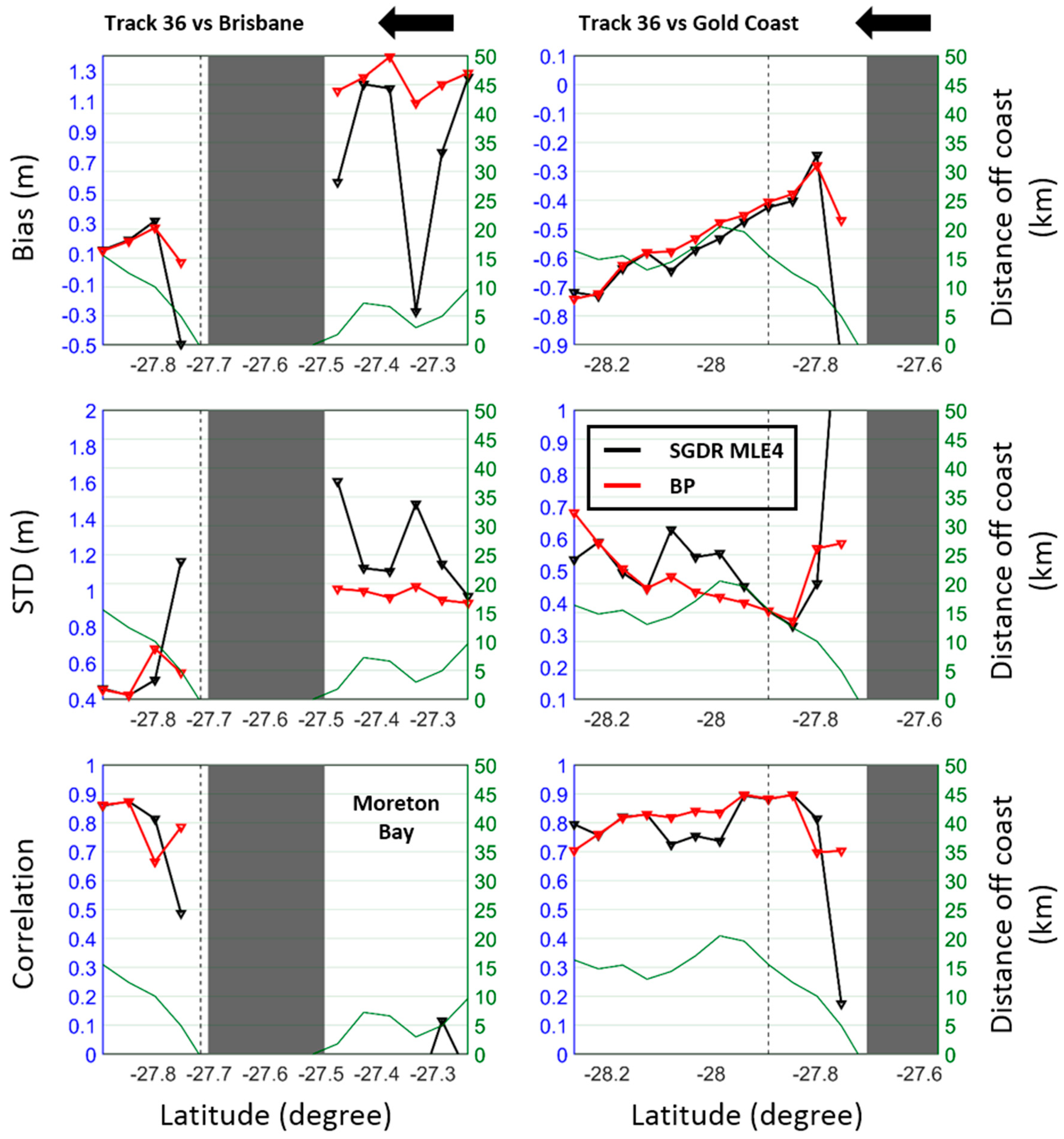
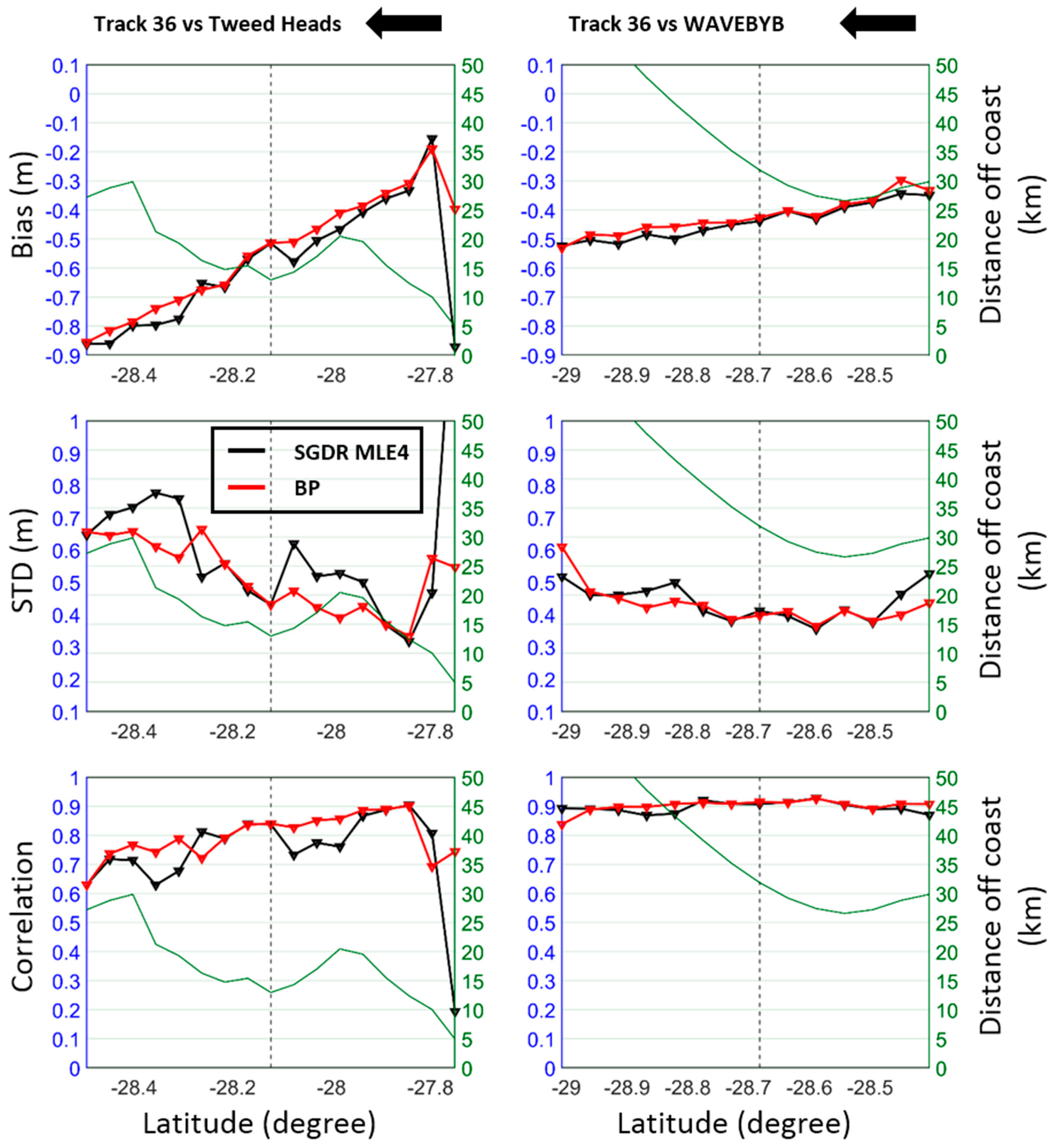
5.4. New South Wales

In this region (Figure 9), the coastline orientation changes from southeastward to southwestward. There are two buoys, about 10–13 km offshore, located at WAVECRH (ca. 31.8°S) and WAVEEND (ca. 37.2°S). The corresponding track 47 moves northeastward nearly parallel to the coastline. The wave climate is predominantly influenced by strong winds on the south coast of Australia [30,31,32].
At WAVECRH (left in Figure 9), both BP and SGDR MLE4 along-track 1 Hz SWHs are almost identical and highly correlated (>0.9) with buoy wave heights, as all along-track points are far away (>50 km) from the coast. When the track moves northeastward, the along-track negative biases slightly change from ca. 0.52 m to ca. 0.58 m, while the STDs increase from ~0.5 m to 0.6 m with a slight quality improvement by the BP discovered around 31.95°S. At WAVEEDN (right in Figure 9), the along-track validation results against buoy SWHs show a similar feature to those in Gold Coast (right in Figure 7), Tweed Heads, and WAVEBYB (Figure 8), that is, the minimum bias (ca. 0.0 ± 0.3 m) is visually reached nearshore rather than near the buoy. Within 8 km from the coast, the degradation of data quality is shown for both the BP and the SGDR MLE4 though the BP’s results appear better than those of the SGDR MLE4. The positive bias is due to the land contamination as mentioned before. However, the high correlation coefficients (>0.9) between the BP and buoy strongly imply the consistency between altimeter estimates and buoy observations in this region.

5.5. Discussion of Common Issues

Because of the temporal and spatial proximity, as well as sampling variability between altimetry and buoy measurement systems, there exists non-negligible differences between observations from both systems. Previous studies [16,17] show that the STD of SWH differences between the two systems can be up to 0.5 m over the open ocean, where both of them are supposed to be well performing. In the coastal region, the STD of differences between altimeter and buoy SWHs becomes even larger due to land contamination and the more energetic environment as shown in Figure 5, Figure 6, Figure 7, Figure 8 and Figure 9. From the analysis of the present study area, we found that along-track STDs of SWH differences between Jason-1 and buoy vary in general from ca. 0.1 m to ca. 0.7 m for both BP and SDGR MLE4 SWHs.
In general, the along-track results show that the BP outperforms the SGDR MLE4 in the 10 km closest to the coast, where the altimeter waveforms are most likely affected by the land returns. We found that if the oceanic waveform is corrupted by the high land reflections or bright target, the off-nadir angle square provided in the SGDR product is usually inaccurate. Using the inaccurate off-nadir angle square degrades the performance of the BP retracker (results not shown). To overcome this problem, research on how the BP retracker can be further improved is still ongoing.
The wave climate along the east coast of Australia is dominated by wind-forced coastal trapped waves, and affected by the coastal morphology such as the Great Barrier Reef and the width of the continental shelf [28,29,30,31,32]. These effects have already been shown in validations in Section 5.1, Section 5.2, Section 5.3 and Section 5.4. Figure 5, Figure 6, Figure 7, Figure 8 and Figure 9 also show that both the BP and SGDR MLE4 data systematically overestimate SWHs in the study area, producing negative biases with respect to the buoy data (i.e., buoy-altimeter), except for the Brisbane station. Similar overestimations have been noted in past validation studies of altimeter SWHs (e.g., Envisat, Jason-1/2, and SARAL/AltiKa) against buoy data [2,5,10,19,26]. For example, the along-track negative biases (ca. 0.1–0.3 m) in the North and Central Queensland coastal areas are in good agreement with those (ca. 0.1–0.5 m) from the validation of Jason-2 coastal wave heights using buoy data by [10]. From the along-track analysis, there is no systematic bias between the BP and SGDR MLE4 SWHs though the improved SWHs by BP can be seen from point to point. This is attributed to the fact that the same σp value was used in the BP and SGDR MLE4.
Over coastal areas for buoys located south of Brisbane including New South Wales (Figure 7, Figure 8 and Figure 9), the along-track biases between altimeter and buoy SWHs tend to become large as tracks move away from the coastline. It can be visually observed that the minimum bias is in general reached at the along-track point close to the coastline rather than at the point closest to the buoy. This raises the question of the cause of this common feature.
This is the area with a narrow continental shelf, where nearshore wave heights are again influenced by wind-forced coastal trapped waves [30,31,32], while offshore wave heights are dominated by synoptic scales [5]. The wave direction is typically opposite to that of Jason-1 track 36 off South Queensland and follows the moving of track 47 off New South Wales [33]. Waves propagating in deep water (~5000 m) in the Tasman Sea rapidly shoal to shallow water (ca. 100 m) at the East Australian shelf [33]. Since buoys are located only a few km offshore between 1.0 and 12.5 km, the local wave climate may be the major cause of smaller biases at the coast and increasing biases offshore. This phenomenon is also seen in the validation of SWHs from the Envisat SGDR and COASTALT products [2]. However, both along-track 1 Hz SWHs from BP and mostly from SGDR MLE4 are in good agreement (correlation > 0.8) with buoy SWHs in this area for distance >10 km offshore. Therefore, we would suggest that the bias between the altimeter and buoy SWHs should be determined from not only the minimum bias value, but also the analysis of the STD and correlation over Eastern Australian coastal areas.

6. Conclusions

This paper addresses the validation of improved SWHs estimated from the reprocessing of three years of Jason-1 satellite altimetric waveforms using the BP retracker along the east coast of Australia. The 1 Hz BP SWHs have been compared with SGDR MLE4 SWHs. Both BP and SGDR MLE4 SWH (1 Hz) datasets have been validated against the independent buoy datasets from eight coastal waverider buoys in the study area. The east coast of Australia has complex coastal morphology and wave climate, which provides a challenging test region to evaluate how much the SWH estimates can be improved by processing coastal waveforms using the BP retracker. The results from this study, in turn, provide an assessment of the superior BP performance in Australian coastal zones.
The evaluation verifies that the BP retracker can provide more reliable SWH estimates than the SGDR MLE4 for nearshore distances 0–12 km and achieve similar performance to the SGDR MLE4 for offshore distance beyond 12 km. The improvement of 1 Hz BP SWHs is clearly demonstrated in terms of data quality and availability, with the lower data noise (STDs between ca. 0.5 and 0.9 m) and the larger percentage (ca. 80%) of retrieved SWHs, when compared with the STDs (between ca. 0.6 and 2.3 m) and ca, 50% of SWHs retrieved by the SGDR MLE4.
The comparison between altimeter SWHs and buoy data shows that both the BP and SGDR MLE4 data tend to overestimate SWHs over the study area. This is consistent with the validation results of altimeter SWHs in coastal regions and open oceans [2,5,10,19,26]. The estimated negative biases have typical values (ca. 0.33 ± 0.50 m) for both BP and SGDR MLE4 within offshore distances of 12–50 km, but they are more precise (ca. 0.21 ± 0.42 m) by the BP than the SGDR MLE4 (ca. 0.33 ± 0.53 m) for nearshore distances of 2–12 km.
The validation of 1 Hz along-track SWHs against buoys further proves the better performance of the BP retracker in extending high quality SWHs from the open ocean toward the coast. The BP achieves smaller biases and STDs, and higher correlation coefficients compared to the SGDR MLE4 in almost all along-track points, except for a few nearshore points.
The validation also reveals two different wave climates over coastal areas north and south of Brisbane. In the North and Central Queensland coastal zones, a combined analysis of the biases, STDs and correlations results in the stable bias estimates ranging from −0.1 m to −0.3 m. At Cairns, the correlation between BP SWHs and buoy values is relatively low with correlation coefficients less than 0.5, which may be explained by the large spatial and temporal variation of coastal wave heights due to the complex air-sea interactions and the existence of the Great Barrier Reef [14,28]. In the South Queensland and New South Wales coastal oceans, we find that the buoy at Brisbane is not adequate for validating Jason-1 SWHs due to complex coastal morphology and different wave conditions in Moreton Bay and surrounding islands. For coastal oceans south of Brisbane, the minimum difference between altimeter and buoy data is often visually reached at the point close to the coastline rather than the point closest to the buoy; and the along-track biases increase as the satellite moves toward the open ocean. This feature may be a combined result of the along-coast wave climate dominated by the wind-forced coastal trapped waves, the synoptic-scale offshore wave system, the width of the continental shelf, and errors in buoy and altimeter data. However, the high and stable correlation (>0.8) between the BP and buoy wave heights are also observed in the coastal zones south of Brisbane, indicating the consistency of the wave heights by the BP and buoys over the continental shelf. In addition, the degradation of some 1 Hz SWHs from the BP suggests that more cautious quality control is needed to avoid spurious data; and a further improvement in the BP retracker is required for coastal SWH applications.
The improvement of the BP retracker is mainly due to its better performance in handling coastal waveforms, which are normally affected by the returns from the land and bright targets. The non-ocean reflections superimposed on the waveform trailing edge cause contaminated coastal waveform shapes. The results from this study reveal that the SWHs provided by the SGDR product are inaccurate within 12 km from the coast, as the adopted MLE4 algorithm, which directly fits the Brown model [21] to the contaminated waveform, cannot accurately resolve parameters. By contrast, our BP retracker can better cope with coastal waveforms due to its feature of weighted estimation (i.e., WLS3) of contaminated waveforms. Therefore, the BP can precisely resolve parameters from the coastal waveforms, and estimate improved SWHs accordingly. Despite the fact that the performance of the BP retracker has so far only been validated around Australia using Jason-1 data [12], we believe that the BP retracker is able to reprocess coastal waveforms elsewhere due to the similar operating principle of different conventional altimeters and diverse coastal topography around Australia. Thus, the BP retracker makes altimeters a valuable component of coastal ocean observing systems [34].
This study shows that the BP retracker can provide more reliable SWH dataset than the standard SGDR product. The BP SWHs can be very useful to monitor the sea state where no buoy SWHs are available and to validate an operational wave model or SWHs from other instruments. An issue found in this study is that the WLS3 estimator may not work well in some coastal zones, because it uses the off-nadir angle included in the SGDR product as one of the initials. Thus, research into further improvement of the BP retracker is currently continuing. One of the limitations in conventional pulse-limited altimeters, such as the Jason-1, is that the altimeter footprint diameter is large, varying from 2 km to 20 km depending on different wave conditions [8,35]. This results in the well-known problem that altimeter returned echoes are often contaminated by the coastal environment. Further improvement requires more advanced altimetry technology, such as the synthetic aperture radar (SAR) mode altimeter (e.g., CryoSat-2 and Sentinel-3A) and the Ka-band altimeter (e.g., SARAL/Altika), which both have shown excellent performance in coastal regions [10,18,35,36,37,38,39].

Author Contributions

F.P. conceived the methods, designed the computer programs, and performed and analysed the experiments. X.D. conceived and supervised the present study, and helped with the discussions and formal analysis of the methods and results, as well as funding acquisition. Both authors contributed to the manuscript writing.

Funding

Australian Research Council Discovery Project DP150100615.

Acknowledgments

This research is supported by the Australian Research Council’s Discovery Project funding scheme (project number DP150100615). The first author is supported by the China Scholarship Council (CSC) Living Allowance Scholarship and University of Newcastle CSC Top Up Scholarship for his PhD study. The author would like to thank Marcello Passaro for his help in reprocessing the SWH data, and Prof. Mark Stewart for kindly reviewing the manuscript. We also thank the anonymous reviewers and the Assistant Editor (Taylor Han) for their comments on this manuscript.

Conflicts of Interest

The authors declare no conflict of interest. The founding sponsors had no role in the design of the study; in the collection, analyses, or interpretation of data; in the writing of the manuscript; or in the decision to publish the results.

References

  1. Bhatt, V.; Kumar, R.; Basu, S.; Agarwal, V.K. Assimilation of altimeter significant wave height into a third-generation global spectral wave model. IEEE Trans. Geosci. Remote Sens. 2005, 43, 110–117. [Google Scholar] [CrossRef]
  2. Caballero, I.; Gómez-Enri, J.; Cipollini, P.; Navarro, G. Validation of high spatial resolution wave data from Envisat RA-2 altimeter in the Gulf of Cádiz. IEEE Geosci. Remote Sens. Lett. 2014, 11, 371–375. [Google Scholar] [CrossRef]
  3. Dufau, C.; Martin-Puig, C.; Moreno, L. User requirements in the coastal ocean for satellite altimetry. In Coastal Altimetry; Vignudelli, S., Kostianoy, A.G., Cipollini, P., Benveniste, J., Eds.; Springer: Berlin/Heidelberg, Germany, 2011; pp. 51–60. [Google Scholar]
  4. Young, I.R. An intercomparison of Geosat, Topex and ERS1 measurements of wind speed and wave height. Ocean Eng. 1998, 26, 67–81. [Google Scholar] [CrossRef]
  5. Passaro, M.; Fenoglio-Marc, L.; Cipollini, P. Validation of significant wave height from improved satellite altimetry in the German Bight. IEEE Trans. Geosci. Remote Sens. 2015, 53, 2146–2156. [Google Scholar] [CrossRef]
  6. Gommenginger, C.; Thibaut, P.; Fenoglio-Marc, L.; Quartly, G.; Deng, X.; Gómez-Enri, J.; Challenor, P.; Gao, Y. Retracking altimeter waveforms near the coasts. In Coastal Altimetry; Vignudelli, S., Kostianoy, A.G., Cipollini, P., Benveniste, J., Eds.; Springer: Berlin/Heidelberg, Germany, 2011; pp. 61–101. [Google Scholar]
  7. Cotton, P.D.; Carter, D.J.T. Cross calibration of TOPEX, ERS-1, and Geosat wave heights. J. Geophys. Res. Oceans 1994, 99, 25025–25033. [Google Scholar] [CrossRef]
  8. Durrant, T.H.; Greenslade, D.J.M.; Simmonds, I. Validation of Jason-1 and Envisat remotely sensed wave heights. J. Atmos. Ocean Technol. 2009, 26, 123–134. [Google Scholar] [CrossRef]
  9. Zieger, S.; Vinoth, J.; Young, I.R. Joint calibration of multiplatform altimeter measurements of wind speed and wave height over the past 20 years. J. Atmos. Ocean Technol. 2009, 26, 2549–2564. [Google Scholar] [CrossRef]
  10. Hithin, N.K.; Remya, P.G.; Nair, T.M.B.; Harikumar, R.; Kumar, R.; Nayak, S. Validation and intercomparison of SARAL/Altika and PISTACH-derived coastal wave heights using in-situ measurements. IEEE J. Sel. Top. Appl. Earth Obs. Remote Sens. 2015, 8, 4120–4129. [Google Scholar] [CrossRef]
  11. Passaro, M.; Cipollini, P.; Vignudelli, S.; Quartly, G.D.; Snaith, H.M. Ales: A multi-mission adaptive subwaveform retracker for coastal and open ocean altimetry. Remote Sens. Environ. 2014, 145, 173–189. [Google Scholar] [CrossRef] [Green Version]
  12. Peng, F.K.; Deng, X.L. A new retracking technique for Brown peaky altimetric waveforms. Mar. Geod. 2018, 41, 99–125. [Google Scholar] [CrossRef]
  13. Gourlay, M.R. Waves, Set-Up and currents on reefs: Cay formation and stability. In Proceedings of the Conference on Engineering in Coral Reef Regions, Townsville, Australia, 1–4 September 1996; pp. 149–264. [Google Scholar]
  14. Gallop, S.L.; Young, I.R.; Ranasinghe, R.; Durrant, T.H.; Haigh, I.D. The large-scale influence of the Great Barrier Reef matrix on wave attenuation. Coral Reefs 2014, 33, 1167–1178. [Google Scholar] [CrossRef] [Green Version]
  15. Shand, T.D.; Wasko, C.D.; Goodwin, I.D.; Carley, J.T.; You, Z.J.; Kulmar, M.; Cox, R.J. Long-term trends in NSW coastal wave climate and derivation of extreme design storms. In Proceedings of the 20th New South Wales Coastal Conference, Tweed Heads, Australia, 10–12 November 2011. [Google Scholar]
  16. Dobson, E.; Monaldo, F.; Goldhirsh, J.; Wilkerson, J. Validation of Geosat altimeter-derived wind speeds and significant wave heights using buoy data. J. Geophys. Res. Oceans 1987, 92, 10719–10731. [Google Scholar] [CrossRef]
  17. Monaldo, F. Expected differences between buoy and radar altimeter estimates of wind speed and significant wave height and their implications on buoy-altimeter comparisons. J. Geophys. Res. Oceans 1988, 93, 2285–2302. [Google Scholar] [CrossRef]
  18. Chaudhary, A.; Basu, S.; Kumar, R.; Prasad, K.V.S.R.; Sharma, R. Retrieving significant wave height in the indian ocean near Visakhapatnam using Jason-2 altimeter data. Remote Sens. Lett. 2015, 6, 286–294. [Google Scholar] [CrossRef]
  19. Queffeulou, P. Long-term validation of wave height measurements from altimeters. Mar. Geod. 2004, 27, 495–510. [Google Scholar] [CrossRef]
  20. Ray, R.D.; Beckley, B.D. Simultaneous ocean wave measurements by the Jason and Topex satellites, with buoy and model comparisons special issue: Jason-1 calibration/validation. Mar. Geod. 2003, 26, 367–382. [Google Scholar] [CrossRef]
  21. Brown, G. The average impulse response of a rough surface and its applications. IEEE Trans. Antennas Propag. 1977, 25, 67–74. [Google Scholar] [CrossRef]
  22. Amarouche, L.; Thibaut, P.; Zanife, O.Z.; Dumont, J.P.; Vincent, P.; Steunou, N. Improving the Jason-1 ground retracking to better account for attitude effects. Mar. Geod. 2004, 27, 171–197. [Google Scholar] [CrossRef]
  23. Thibaut, P.; Amarouche, L.; Zanife, O.Z.; Steunou, N.; Vincent, P.; Raizonville, P. Jason-1 altimeter ground processing look-up correction tables. Mar. Geod. 2004, 27, 409–431. [Google Scholar] [CrossRef]
  24. Thibaut, P.; Poisson, J.C.; Bronner, E.; Picot, N. Relative performance of the MLE3 and MLE4 retracking algorithms on Jason-2 altimeter waveforms. Mar. Geod. 2010, 33, 317–335. [Google Scholar] [CrossRef]
  25. Caires, S.; Sterl, A. Validation of ocean wind and wave data using triple collocation. J. Geophys. Res. Oceans 2003, 108. [Google Scholar] [CrossRef] [Green Version]
  26. Caires, S.; Sterl, A.; Bidlot, J.R.; Graham, N.; Swail, V. Intercomparison of different wind–wave reanalyses. J. Clim. 2004, 17, 1893–1913. [Google Scholar] [CrossRef]
  27. Hemer, M.A.; Church, J.A.; Hunter, J.R. Waves and climate change on the Australian coast. J. Coast. Res. 2007, 50, 432–437. [Google Scholar]
  28. Middleton, J.H. Low-frequency trapped waves an a wide, reef-fringed continental shelf. J. Phys. Oceanogr. 1983, 13, 1371–1382. [Google Scholar] [CrossRef]
  29. Middleton, J.H.; Cunningham, A. Wind-forced continental shelf waves from a geographical origin. Cont. Shelf Res. 1984, 3, 215–232. [Google Scholar] [CrossRef]
  30. Church, J.A.; Freeland, H.J. The energy source for the coastal-trapped waves in the Australian coastal experiment region. J. Phys. Oceanogr. 1987, 17, 289–300. [Google Scholar] [CrossRef]
  31. Church, J.A.; Freeland, H.J.; Smith, R.L. Coastal-trapped waves on the east Australian continental shelf part i: Propagation of modes. J. Phys. Oceanogr. 1986, 16, 1929–1943. [Google Scholar] [CrossRef]
  32. Church, J.A.; White, N.J.; Clarke, A.J.; Freeland, H.J.; Smith, R.L. Coastal-trapped waves on the east Australian continental shelf part ii: Model verification. J. Phys. Oceanogr. 1986, 16, 1945–1957. [Google Scholar] [CrossRef]
  33. Mortlock, R.T.; Goodwin, D.I. Directional wave climate and power variability along the Southeast Australian shelf. Cont. Shelf Res. 2015, 98, 36–53. [Google Scholar] [CrossRef]
  34. Liu, Y.; Kerkering, H.; Weisberg, R.H. (Eds.) Coastal Ocean Observing Systems; Elsevier: London, UK, 2015; p. 461. [Google Scholar]
  35. Chelton, D.B.; Walsh, E.J.; MacArthur, J.L. Pulse compression and sea level tracking in satellite altimetry. J. Atmos. Ocean. Technol. 1989, 6, 407–438. [Google Scholar] [CrossRef]
  36. Fenoglio-Marc, L.; Dinardo, S.; Scharroo, R.; Roland, A.; Sikiric, M.D.; Lucas, B.; Becker, M.; Benveniste, J.; Weiss, R. The German Bight: A validation of Cryosat-2 altimeter data in SAR mode. Adv. Space Res. 2015, 55, 2641–2656. [Google Scholar] [CrossRef]
  37. Phalippou, L.; Enjolras, V. Re-tracking of SAR altimeter ocean power-waveforms and related accuracies of the retrieved sea surface height, significant wave height and wind speed. In Proceedings of the 2007 IEEE International Geoscience and Remote Sensing Symposium, Barcelona, Spain, 23–28 July 2007; pp. 3533–3536. [Google Scholar]
  38. Sepulveda, H.H.; Queffeulou, P.; Ardhuin, F. Assessment of SARAL/Altika wave height measurements relative to buoy, Jason-2, and Cryosat-2 data. Mar. Geod. 2015, 38, 449–465. [Google Scholar] [CrossRef]
  39. Shaeb, K.H.B.; Anand, A.; Joshi, A.K.; Bhandari, S.M. Comparison of near coastal significant wave height measurements from SARAL/Altika with wave rider buoys in the Indian region. Mar. Geod. 2015, 38, 422–436. [Google Scholar] [CrossRef]
Figure 1. The location of waverider buoys (red inversed triangles) and corresponding Jason-1 ground tracks (black lines). The four areas from upper left to bottom right are called hereafter as North Queensland, Central Queensland, South Queensland, and New South Wales, respectively. The blue box in the inset indicates the corresponding area in Australia. For validation, altimetry data within 50 km from the buoys are analysed.
Remotesensing 10 01072 g001
Figure 2. Comparison between retracked SWHs from the BP and the SGDR MLE4 based on the distance to the coast. (a) The mean STDs of 20 Hz SWHs; (b) The mean number of 20 Hz SWHs; (c) The total number of retrieved 1 Hz SWHs; (d) The percentage of retrieved 1 Hz SWHs.
Remotesensing 10 01072 g002
Figure 3. Scatter plots of pairs of 1 Hz BP and buoy SWHs according to the distance from the coast: (a) 12–50 km and (b) 0–12 km. The red line represents the linear relationship between these two datasets. The black line depicts the ideal situation that altimeter and buoy SWHs are the same with the unity slope.
Remotesensing 10 01072 g003
Figure 4. Similar to Figure 3, but for the results from the SGDR MLE4.
Remotesensing 10 01072 g004
Figure 5. Validation of 1 Hz along-track SWHs for tracks 175 (left) and 214 (right) against buoy SWHs at Cairns in North Queensland in terms of point-wise bias, STD and correlation coefficients. The 1 Hz SWHs are derived from the SGDR MLE4 (black) and BP (red) retracker. The black arrow on the top indicates the flight direction of the satellite. The grey area indicates the land, and the green line represents the distance of the along-track points off the coast. The black vertical dash line denotes the closest point of the track from the buoy.
Remotesensing 10 01072 g005
Figure 6. Similar to Figure 5, but for tracks 36 (left) and 149 (right) against buoy SWHs at Gladstone in Central Queensland.
Remotesensing 10 01072 g006
Figure 7. Similar to Figure 5, but for tracks 36 against buoy SWHs at Brisbane (left) and Gold Coast (right) in South Queensland. The correlation (bottom in left panel) is not computed and shown, as the number of SWHs at the point is less than 30.
Remotesensing 10 01072 g007
Figure 8. Similar to Figure 5, but for tracks 36 against buoy SWHs at Tweed Heads (left) and WAVEBYB (right) in South Queensland.
Remotesensing 10 01072 g008
Figure 9. Similar to Figure 5, but for track 47 against buoy SWHs at WAVECRH (left) and WAVEEDN (right) in New South Wales.
Remotesensing 10 01072 g009
Table 1. Description of buoys and corresponding altimeter tracks.
BuoyAltimeter TrackMinimum Buoy-Track Distance (km)Maximum Buoy-Track Distance (km)Buoy-Coast Distance (km)
Cairns17544.849.62.2
2149.746.42.2
Gladstone3617.145.95.0
14912.649.75.0
Brisbane3623.847.110.1
Gold Coast3614.945.01.1
Tweed Heads3612.348.51.6
WAVEBYB3632.949.55.6
WAVECRH4744.049.810.0
WAVEEDN477.046.912.5

