Sea Surface Monostatic and Bistatic EM Scattering Using SSA-1 and UAVSAR Data: Numerical Evaluation and Comparison Using Different Sea Spectra

Abstract

The microwave scatterometer is one of the most effective instruments in ocean remote sensing, which urges the need for some theoretical models to accurately estimate the scattering coefficient of the sea surface. For the simulation of the scattering from an ocean surface, the sea spectrum, or its inverse Fourier transform, autocorrelation function is essential. Currently, many sea spectral models have been proposed for describing sea waves. However, which spectrum should be adopted during electromagnetic (EM) computations? A systematic comparison of these models is needed to evaluate their accuracies. In this paper, we focus on numerical simulations of scattering from a rough sea surface in monostatic and bistatic configurations by using six different sea spectral models and the first-order small slope approximation (SSA-1). First, sea spectral models proposed by Elfouhaily et al., Hwang et al., Romeiser et al., Apel et al., Fung et al., and Pierson et al., are compared with each other from different points of view, e.g., the omnidirectional parts, the angular spreading functions, the autocorrelation functions, and the slope variances. We find that the spectra given by Elfouhaily and Hwang could reflect realistic wind sea waves more accurately. Then, the scattering coefficients are simulated in fully monostatic and bistatic configurations. Regarding the monostatic scattering, the results simulated using EM scattering models are compared with those obtained from the measured UAVSAR data in the L band and the empirical model CMOD5 in the C band. Comparisons are made for various incident angles, wind speeds, and wind directions. Meanwhile, special attention is paid to low to moderate incident angles. The comparisons show that, it is difficult to find one certain spectral model to simulate scattering coefficient accurately under all wind speeds or wind directions. Accurate estimations will be obtained using different methods according to different situations.

1. Introduction

The microwave scatterometer is one of the most effective instruments in ocean remote sensing since it can provide valuable measurements at both day and night in spite of the atmospheric conditions. In the past decades, many microwave radars that operate at various frequencies have been developed for airborne and space-borne platforms, such as the Advanced Synthetic Aperture Radar (ASAR) on the European Space Agency (ESA)’s ENVISAT-1 satellite, which was launched in 2002; the Phased-Array L-Band Synthetic Aperture Radar (PALSAR) on the Advanced Land Observing Satellite (ALOS), which was launched in 2006; synthetic aperture radar on the Canadian Space Agency’s Radarsat-1 and Radarsat-2, which were launched in 1995 and 2007, respectively; and synthetic aperture radar carried on the Sentinel-1 satellite launched in 2014 by the European Space Agency. These radars have been proven to be useful tools for ocean observations, e.g., sea wave retrieval, wind speed retrieval, ship detection, oil spill monitoring, etc. Among these applications, the estimation of scattering coefficient (σ₀ or NRCS, normalized radar cross-section) from sea clutter is of critical importance. Thus, it is required to develop accurate (theoretical or empirical) models to predict the radar scattering coefficient of the sea background.

At present, geophysical model functions (GMFs), such as CMOD5 for the C band, NSCAT2 for the Ku band, etc., are often employed in ocean remote sensing. These GMFs have been widely used in ocean wind field retrieval. It also has been proven that GMFs can provide accuracy predictions in practical applications. However, just like all other empirical models, GMFs have no physical meaning, which make it impossible for more physical interpretations. Therefore, it is necessary to develop theoretical models for simulating the scattering from the sea surface. When dealing with the problem of scattering from a rough surface, it is known that there is no exact analytical solution for the scattering field. In the past decades, various approximate methods have been proposed to overcome this difficulty [1]. The most significant among these methods are the Kirchhoff-Tangent Plane Approximation (KA) [2] and the small perturbation method (SPM) [3]. The combination of KA and SPM, which is named the two-scale model (TSM), is also an effective method for calculating the scattering coefficient. Unfortunately, these three methods are available in specific conditions or involve a cutoff parameter to separate sea waves into small and large scales. The small slope approximation proposed by Voronovich [4,5,6] is a unifying model that could reconcile KA and SPM without introducing any arbitrary parameters. SSA has been proved as an appropriate method for large-, intermediate-, and small-scale roughness surfaces under the condition that the tangent of grazing angles of incident/scattered waves is sufficiently larger than the RMS (root mean square) slopes of the rough surface. These approximate methods have been studied and analyzed in the comparisons with the measured radar data [7].

In the evaluations of EM scattering using approximate methods, either the sea spectrum or surface elevation autocorrelation function is essential for scattering coefficient estimation. For microwave scattering, short gravity and capillary-gravity waves serve as roughness elements. Hence, special attention should be paid to the description of the small-scale waves. In this paper, we only discuss the spectra which could provide descriptions for short waves rather than those who could only describe large-scale waves (such as PM spectrum, JONSWAP spectrum). In the past decades, many spectral models that can be used to describe the small-scale waves have been proposed, for instance, the Pierson spectrum [8,9], Bjerkaas and Riedel spectrum [10], Fung spectrum [11], Donelan and Pierson spectrum [12], Apel spectrum [13], Romeiser spectrum [14], Elfouhaily spectrum [15], and Hwang spectrum [16,17,18,19]. These spectral models have been employed in EM computations as they have defined the high-frequency spectra.

Among these spectral models, more attention should be paid onto the Elfouhaily and Hwang spectra. The Elfouhaily spectrum is a unified spectrum that has been studied in many papers. This spectrum is established based on available field and tank measurements. For the low-frequency part, the Elfouhaily spectrum is consistent with the Donelan spectrum [12]. For the high-frequency part, it is consistent with tank measurements. Moreover, the unified spectrum takes into account the influences caused by wind fetch on the wave behaviors. With respect to the Hwang spectrum, it is a very new spectrum which is derived based on the analysis of the wave action balance function and field measurements. The curvature spectrum is expressed as $B\left(k\right)=A\left(k\right){\left(u_{*}/c\right)}^{a\left(k\right)}$, where $u_{*}$ is the friction velocity, c is the phase speed of wave, and k denotes the wavenumber. A(k) and a(k) are given as polynomial fitting functions.

A reliable spectrum is of crucial importance for predicting the scattering coefficients precisely. Up to now, on the basis of different sea spectral models, many works about EM computations of the sea surface have been carried out. Voronovich et al. studied the scattering from the sea surface with breaking waves with SSA and the Elfouhaily spectrum in the Ku- and C-bands [5]. Awada et al. conducted comparisons between the results estimated using the first-order SSA, the TSM model, and the Elfouhaily spectrum in the bistatic configuration [20]. Ayari et al. studied the bistatic scattering of the sea surface using TSM and the Elfouhaily spectrum. In their work, the scattering coefficients calculated with TSM and the Elfouhaily spectrum were compared with those obtained with CMOD5, SSA, and the Pierson spectrum [21]. Du et al. studied the backscattering from the sea surface with the advanced integral equation method, an improved angular spreading function, and Apel’s omnidirectional spectrum [22]. Additionally, the sea spectral model can also be used to study the nonlinear and non-spectral ocean surface effects (including Doppler-induced effects and rapid changes on the surface) [23,24]. However, most of the previous papers focus on only one or two spectral models. To the best of our knowledge, few comprehensive comparison studies of these spectral models have been reported, especially for the application of ocean remote sensing. In this context, a systematic study of different sea spectra has been conducted in this work.

The rest of this paper is organized as follows: in Section 2, spectral models proposed by different researchers are reviewed and compared with each other. In Section 3, theoretical derivations of SSA-1 and CMOD5 are briefly reviewed. Section 4 is dedicated to some numerical simulations in monostatic and bistatic configurations, which are analyzed as functions of several parameters: incident angle, wind speed, wind direction, scattering angle, and scattering azimuth angle. The meaningful conclusions are drawn in the final section.

2. Sea Spectrum

In general, sea surface waves are considered as an ergodic and stationary random process and the sea spectrum is often used to describe them. The sea spectrum is one of the two order statistical properties of sea waves and it can be directly obtained by the inverse Fourier transformation of the sea surface height’s autocorrelation. In order to study the scattering from the sea surface, it is necessary to get enough knowledge of the sea spectrum. This part aims at presenting different sea spectra and discussing the differences between them. For convenience’s sake, in the following, we denote the spectrum proposed by Elfouhaily et al. [15] as the E-spectrum, the spectrum proposed by Hwang et al. [16,17,18,19] as the H-spectrum, the spectrum proposed by Romeiser et al. [14] as the R-spectrum, the spectrum proposed by Apel et al. [13] as the A-spectrum, the spectrum proposed by Fung et al. [11] as the F-spectrum, the spectrum proposed by Pierson et al. [9] as the P-spectrum, respectively.

A sea spectrum describes the distribution of each harmonic component of the sea surface as function of the spatial wavenumber and wind direction. Usually, it can be expressed as:

$$S(k,\varphi )=S_0\left(k\right)\cdot f(k,\varphi ),$$

(1)

where $S_0\left(k\right)$ represents the omnidirectional part, and $f(k,\varphi )$ represents the angular spreading function. k and $\varphi$ are the spatial wave number and the wind direction, respectively.

2.1. Omnidirectional Part of Sea Spectra

Figure 1, Figure 2 and Figure 3 show the omnidirectional parts of the six spectra mentioned above. The wind speeds at 10 m height above sea surface (U₁₀) are 5 m/s, 10 m/s and 15 m/s, respectively. For E-spectrum and H-spectrum, the simulations are performed for an inverse wave age of 0.84, corresponding to a fully-developed sea. In Figure 1a, Figure 2a and Figure 3a, one can observe that different spectral models have similar behaviors. For microwave scattering from the rough sea surface, the primary contribution of the scattering is from the small-scale Bragg resonant waves. A common scatterometer typically operates at a moderate incident angle between about 20° and 60°. To better exhibit the differences between the various sea spectra in the small scale range, Figure 1b, Figure 2b and Figure 3b present the sea spectra that accounts for Bragg scattering for incident angles between about 20° and 60° in the C band, corresponding to the curves within the rectangles of Figure 1a, Figure 2a and Figure 3a. Significant discrepancies can be observed among these the spectral models in this range. Moreover, in Figure 1b, Figure 2b and Figure 3b, the effects of wind speed on different spectral models are also different. The F-spectrum presents almost the same as the P-spectrum since the underlying formulations for the two spectra are identical for this range. Additionally, the spectral energies of the F-spectrum and P-spectrum are larger than other spectra in this range.

2.2. Angular Spreading Function

Since a directional spectrum is the Fourier transform of the two-dimensional covariance of surface elevation, directional spectrum should be a real and even function. Therefore, the Fourier series expansion of an angular spreading function must contain only even harmonics. Unfortunately, some angular spreading functions do not meet this requirement. To solve this problem, Elfouhaily et al. proposed to calculate the angular spreading function with the following expression [15]:

$$f\left(k,\varphi \right)=\frac{1}{2\pi }\left[1+\Delta \left(k\right)\times \cos \left(2\varphi \right)\right].$$

(2)

The term Δ(k) ratio is calculated with:

$$\Delta \left(k\right)=\frac{f^{\prime }\left(k,0\right)-f^{\prime }\left(k,\pi /2\right)}{f^{\prime }\left(k,0\right)+f^{\prime }\left(k,\pi /2\right)},$$

(3)

where $f^{\prime }\left(k,\varphi \right)$ denotes the angular spreading functions proposed by different authors [25]. For the sake of simplicity, the explicit formulas for them are not given here, but the numerical simulations are shown in Figure 4.

Figure 4 shows the Δ(k) ratios and Figure 5 presents the angular spreading functions based on various formulas, where 0° corresponds to upwind direction and 180° corresponds to downwind direction. Generally, the long wind waves are assumed to be aligned with the mean wind direction in the steady condition, which makes f′ (k, π/2) approaches to zero. As a consequence, Δ(k) should be equal to 1 for large-scale waves. As shown in Figure 4, the Fung and Romeiser angular spreading functions cannot satisfy this requirement. The shorter wind waves are more non-directional, some of them may even travel perpendicular to the wind direction [15].

Combining Figure 4a–c, the wind speed has no influence on Pierson and Apel spreading functions. For Romeiser angular spreading function, the influence of wind on Bragg scattering wave range is quite small. However, in the case of Elfouhaily and Fung functions, the Δ(k) ratios of the Bragg scattering wave range increase with wind speed, which means that the high-frequency waves become more directional in high wind speed conditions.

In Figure 5, all curves have their maximum value in upwind and downwind directions, while reaching their minimum value in the crosswind direction. The value of the Pierson function is zero in the crosswind direction, which means that there is no component perpendicular to the wind direction for k = 135 rad/m, which is not consistent with the real case.

2.3. Slope Variation

The slope variance is regarded as a measurement of sea surface roughness, which can be obtained through the following integrations:

$${\sigma }_u^2={\displaystyle {\int }_0^{\infty }{\displaystyle {\int }_0^{2\pi }{\left(k\cos \varphi \right)}^{2}S\left(k,\varphi \right)}d\varphi dk}$$

(4)

$${\sigma }_c^2={\displaystyle {\int }_0^{\infty }{\displaystyle {\int }_0^{2\pi }{\left(k\sin \varphi \right)}^{2}S\left(k,\varphi \right)}d\varphi dk}$$

(5)

where u denotes upwind direction and c denotes crosswind direction. It can be recognized that the slope variances of upwind and crosswind directions are highly sensitive to the shape of spectra. According to the Cox and Munk model, the slope variances of the upwind and crosswind directions are given as [26]:

$${\sigma }_u^2=\left(5.0+0.78U_{12.5}\right)\times {10}^{-3}$$

(6)

$${\sigma }_c^2=\left(3.0+0.84U_{12.5}\right)\times {10}^{-3}$$

(7)

where U_12.5 is the wind speed at 12.5 m height above sea surface. In the following, the RMS slopes evaluated based on spectral models are compared with the Cox and Munk model.

Figure 6 shows the RMS slopes estimated as functions of wind speeds. For the H-spectrum, the same angular spreading function of E-spectrum is used in this paper. Both for upwind and crosswind directions, one can note that the RMS slopes increase with wind speed. The sea surface becomes rougher under higher wind speed conditions, which corresponds to the real situation. The RMS slopes calculated with E-spectrum and H-spectrum match well with Cox and Munk model both in upwind and crosswind directions. R-spectrum agrees well with Cox and Munk model only in upwind direction. The errors in crosswind direction may be caused by that the angular spreading function cannot describe the real situation accurately. With respect to other spectral models, there exist larger discrepancies with the Cox and Munk curves.

2.4. Autocorrelation Function

The autocorrelation of the displacement field of sea surface, which corresponding to the inverse Fourier transform of the sea spectrum. It describes the correlations between two arbitrary points on a rough surface. The correlation length and the autocorrelation function shape are closely related to the roughness of the rough surface [27]. It is interesting to compare autocorrelation functions calculated based on different sea spectra since they will be employed in calculating the scattering coefficients with SSA-1.

In Figure 7, the autocorrelation functions are normalized by height variances. From this simulation, one can see that the autocorrelation functions calculated based on the E-, A-, and F-spectra almost overlap with each other, while the other two autocorrelation functions exhibit larger differences. The Hwang and Romeiser autocorrelation functions approach zero more slowly. Additionally, with the increase in wind speed, all the curves approach zero more slowly, which indicates that the correlation becomes longer.

3. Models for Scattering Coefficient Estimation

In this part, SSA-1, CMOD5, and the polarization ratio model, which will be applied in the following numerical simulations, are briefly reviewed.

3.1. The First-Order Small Slope Approximation (SSA-1)

The small slope approximation proposed by Voronovich is valid for the arbitrary wavelength, provided the tangent of the grazing angles of the incident/scattered waves sufficiently exceeds the RMS slopes of roughness [4,6]. A noticeable advantage of SSA is that SSA does not involve any arbitrary parameter to separate sea waves into larger and smaller scales. Compared with the second-order SSA (SSA-2), SSA-1 involves a small calculating quantity. Thus, SSA-1 is used in our simulation to simplify the computation. In the following, the calculation procedures for the scattering coefficient with the sea spectra are presented.

The scattering coefficient of SSA-1 can be expressed as [4,5]:

$$\begin{array}{ll}{\sigma }_{\alpha {\alpha }_0}^{SSA-1}\left(k,k_0\right)& =\frac{1}{\pi }{\left|\frac{2q_k{q}_0}{q_k+q_0}{B}_{\alpha {\alpha }_0}\left(k,k_0\right)\right|}^2\exp \left[-{\left(q_k+q_0\right)}^2\rho \left(0\right)\right]\\ & \times {\displaystyle \int \left\{\exp \left[{\left(q_k+q_0\right)}^2\rho \left(r\right)\right]-1\right\}\exp \left[-i\left(k-k_0\right)\cdot r\right]}dr\end{array},$$

(8)

where α and α₀ correspond to the polarizations of scattered and incident waves, respectively. $\alpha {\alpha }_0\in \left\{\mathrm{HH},\mathrm{HV},\mathrm{VH},\mathrm{VV}\right\}$, where H denotes the horizontal polarization and V denotes the vertical polarization. $k_0$ and $k$ are horizontal projections of the vector of incident and scattered waves, respectively. $q_0$ and $q_k$ are the vertical projections of the incident and scattered wave vectors, respectively.

Using the Bessel function, we can obtain the following expression for scattering coefficient [20]:

$${\sigma }_{\alpha {\alpha }_0}^{SSA-1}\left(k,k_0\right)=8{\left|\frac{q_k{q}_0}{q_k+q_0}{B}_{pq}\left(k,k_0\right)\right|}^2\times {\displaystyle {\int }_0^{\infty }rdr\left\{{\exp }^{-{\left(q_k+q_0\right)}^2\left[\rho \left(0\right)-\rho \left(r\right)\right]}-{\exp }^{-{\left(q_k+q_0\right)}^2\rho \left(0\right)}\right\}{J}_0\left(Mr\right)}.$$

(9)

In the above equation, J₀(·) denotes the Bessel function of the first kind of zero-order. $M=k\sqrt{{\left(\sin {\theta }_s\cos {\varphi }_s-\sin {\theta }_i\cos {\varphi }_i\right)}^2+{\left(\sin {\theta }_s\sin {\varphi }_s-\sin {\theta }_i\sin {\varphi }_i\right)}^2}$. θ_i and θ_s represent the incident and the scattered angles. $\rho \left(r\right)$ is the autocorrelation function, ${\varphi }_i$ and ${\varphi }_s$ denote incident and scattered azimuth angles. More details about the derivations can be found in Appendix A.

The calculation of two dimension autocorrelation function can be conducted easily with the help of the Bessel function, which can be expressed as follows [20,28]:

$$\rho \left(r\right)=\rho (r,\varphi )={\rho }_0\left(r\right)-\cos \left(2\varphi \right)\times {\rho }_2\left(r\right),$$

(10)

$$\{\begin{array}{c}{\rho }_0\left(r\right)={\displaystyle {\int }_0^{\infty }{S}_0\left(k\right)J_0\left(kr\right)dk}\\ {\rho }_2\left(r\right)={\displaystyle {\int }_0^{\infty }{S}_0\left(k\right)J_2\left(kr\right)\Delta \left(k\right)dk}\end{array}.$$

(11)

In Equation (11), $J_2(\cdot )$ is the first kind Bessel function of second order. $S_0\left(k\right)$ denotes the omnidirectional part of sea spectrum mentioned in Equation (1), $\Delta \left(k\right)$ can be calculated according to Equation (3) based on the angular spreading functions given by different authors.

Additionally, to model the sea dielectric constant, the Debye equation [29] is employed in all of the following simulations, where the temperature equals 20 °C and salinity equals 35 ppt.

3.2. Empirical Model CMOD5 and PR (Polarization Ratio) Model

In order to quantitatively evaluate the quality of the numerical results simulated by different models, the C band (5.3 GHz) empirical model CMOD5 is introduced in this part. The C band GMF CMOD5 is derived based on a large number of measurements [30]. It has been employed in many studies to retrieve the wind speed of the sea surface or to study the backscattering from the sea surface [31,32,33]. Thus, CMOD5 can be regarded as a reliable reference. The form of the CMOD5 model is given by Equation (12). More details about CMOD5 are presented in [30]:

$${\sigma }_0^{\mathrm{VV}}=B_0{\left(1+B_1\cos \varphi +B_2\cos 2\varphi \right)}^{1.6}$$

(12)

where ${\sigma }_0^{\mathrm{VV}}$ denotes the VV polarized NRCS. It should be noted that the CMOD5 model is only valid for the VV polarized channel in the C band. In order to estimate the scattering coefficient in HH channel, polarization ratio (PR) models are often employed to convert the scattering coefficient from the VV polarization to the HH polarization.

A PR model is commonly defined as:

$$PR=\frac{{\sigma }_0^{\mathrm{VV}}}{{\sigma }_0^{\mathrm{HH}}}$$

(13)

where ${\sigma }_0^{\mathrm{HH}}$ denotes the HH polarized NRCS. In this work, the PR model given by Liu et al. is used which is given as [34]:

$$PR=A\exp \left(B{\theta }_i\right)+C$$

(14)

with A = 0.453041, B = 0.0324573, C = 0.524303. It is noteworthy that empirical approaches do not have any physical meaning, which makes it impossible for physical interpretation.

4. Numerical Simulation and Discussion

4.1. Scattering from the Sea Surface in the Monostatic Configuration

Since most of the current microwave scatterometers measure in the backscattered direction (monostatic case), this makes the problem of EM scattering in the monostatic configuration become a practically meaningful problem. In this context, we first deal with the monostatic configuration. In the following, on the basis of the theories in Section 2, we present some numerical simulations by using SSA-1 and different sea spectra in the fully-monostatic configuration. The scattering coefficients evaluated with SSA-1 and different spectral models are compared with the UAVSAR data in the L band and the empirical model CMOD5 in the C band, respectively.

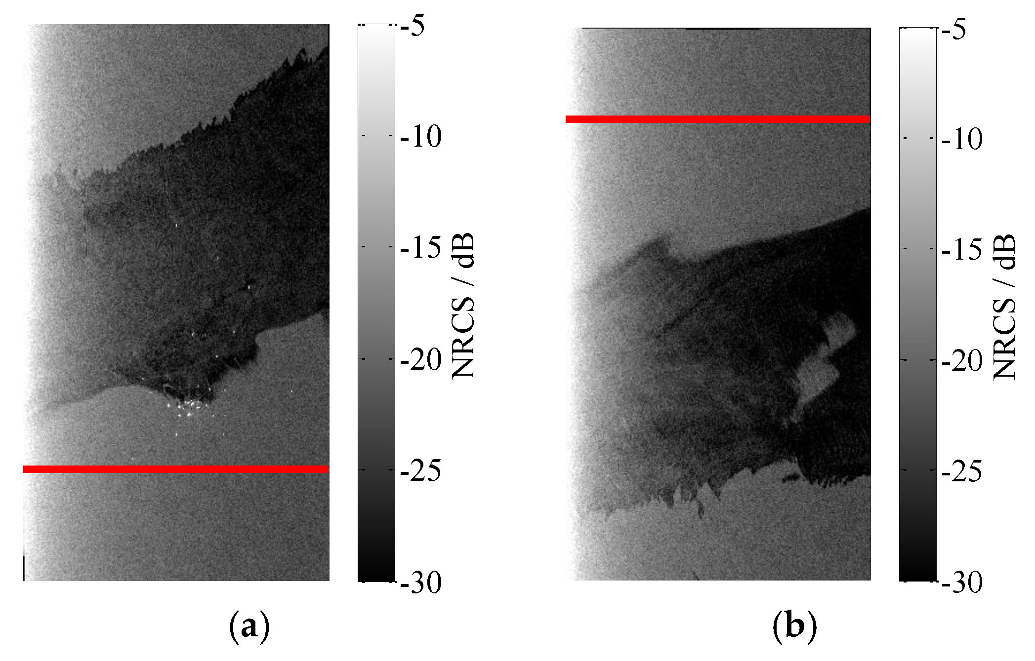
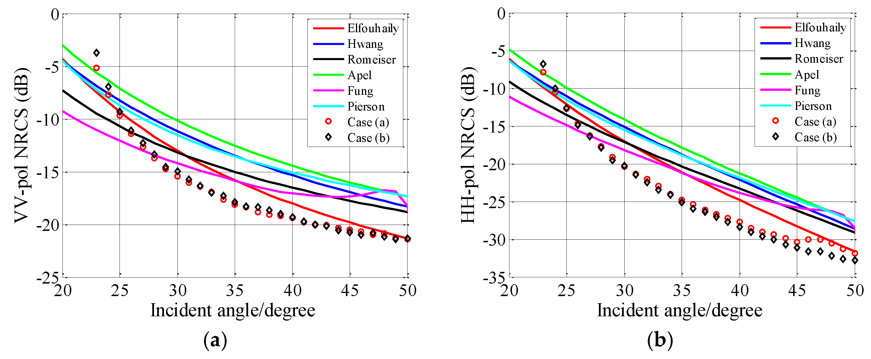
4.1.1. Evaluation with UAVSAR Data in the L Band

The SAR images are collected by UAVSAR (uninhabited aerial vehicle synthetic aperture radar) during the DWH (Deepwater Horizon) oil spill accident in the Gulf of Mexico in 2010. UAVSAR is a fully-polarimetric L-band SAR. The center frequency of the incident wave is 1.2575 GHz. Two multi-look (3 and 12 looks in the range and azimuth directions, respectively) UAVSAR images with a 5 m slant range resolution and 7.2 m azimuth resolution are employed in this part. The two SAR images were acquired from two adjacent, overlapping flight tracks that covered the main oil spills in the Gulf of Mexico. The two flight lines are gulfco_14010_10054_100_100623 (hereafter denoted as Case (a)) and gulfco_32010_10054_101_100623 (hereafter denoted as Case (b)), respectively. The approximate latitudes and longitudes of Case (a) are (30°9′N, 89°54′W) for the upper left pixel, (30°17′N, 89°43′W) for the upper right pixel, (28°19′N, 88°9′W) for the lower left pixel, and (28°26′N, 87°59′W) for the lower right pixel. The approximate latitudes and longitudes of Case (b) are (30°1′N, 90°1′W) for the upper left pixel, (30°9′N, 89°50′W) for the upper right pixel, (28°25′N, 88°28′W) for the lower left pixel, and (28°33′N, 88°17′W) for the lower right pixel. More information about the data are summarized in

Table 1. UAVSAR data information.

Case	Data ID	Time of Acquisition	Incident Angle (°)	Wind Speed U10 (m/s)	Wind Direction (°)
(a)	14010	20:42 UTC 23 June 2010	22–65	2.5–5	115–126
(b)	32010	21:08 UTC 23 June 2010	22–65	2.5–5	115–126

[35].

Figure 8 shows the UAVSAR images. The dark areas are the oil spills induced by the accident. Only the scattering coefficients of the clean sea are used in this work. In order to compare the simulated results with measured data, UAVSAR data are processed as follows: firstly, a 100 × 3300 matrix is obtained by extracting 100 rows of pixels along the red lines in Figure 8. Then, a 1 × 3300 array can be obtained by computing the mean value of each column. Finally, the mean value is calculated in each 1° incident angle range.

Figure 9 presents the NRCSs evaluated with SSA-1 and UAVSAR images. The difference of the observation direction between these two SAR images is about 180°. Therefore, the difference of the wind direction between these two SAR images is about 180°. In our simulations, the wind speed is set as 5 m/s, and the wind direction is set as the upwind direction. In Figure 9, one can note that the difference between the NRCSs acquired from the two SAR images is quite small. Both for VV and HH polarizations, the scattering coefficients evaluated with SSA-1 are larger than the measured SAR data. Obviously, none of the curves coincide well with UAVSAR data. Relatively speaking, the curve of the E-spectrum is slightly better than other curves (the difference between Elfouhaily curve and SAR data curves is less than 3 dB for VV polarization, and 4 dB for HH polarization). For the F-spectrum, there exist oscillations for the incident angle larger than 45° which are caused by the integration of the oscillation function in Equation (8).

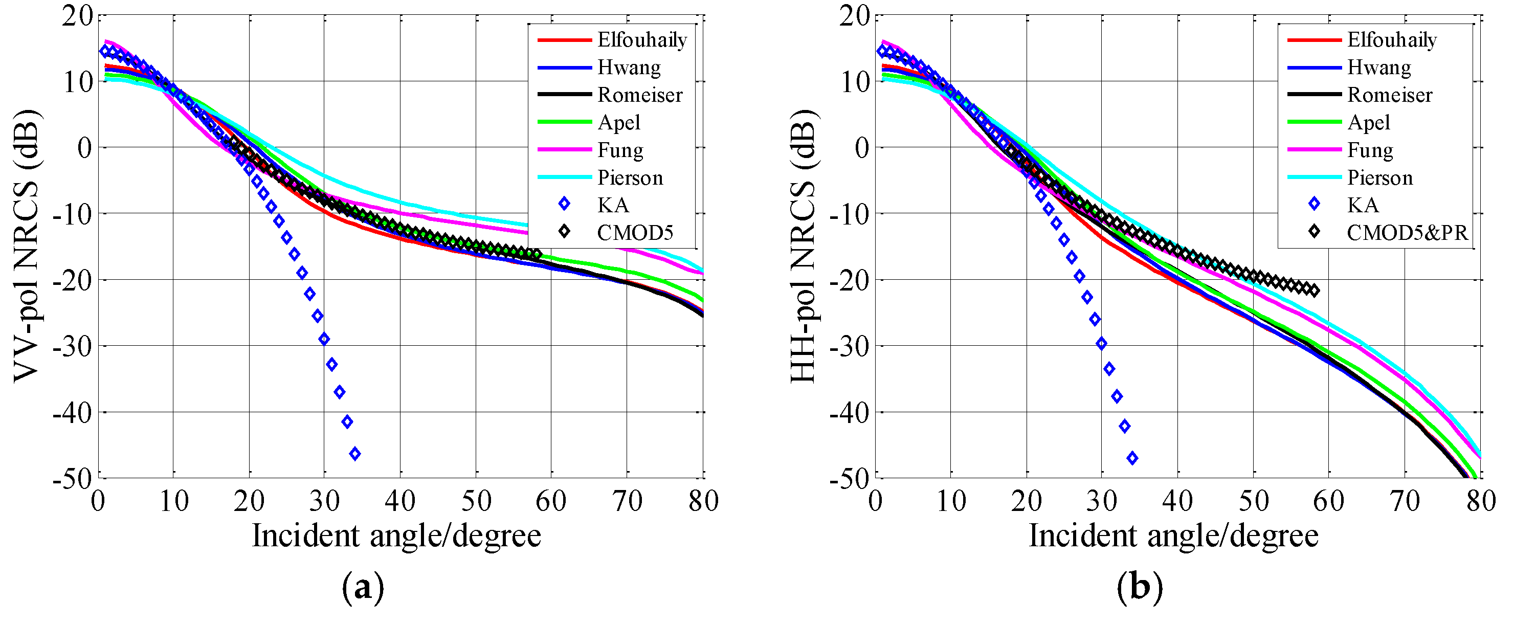
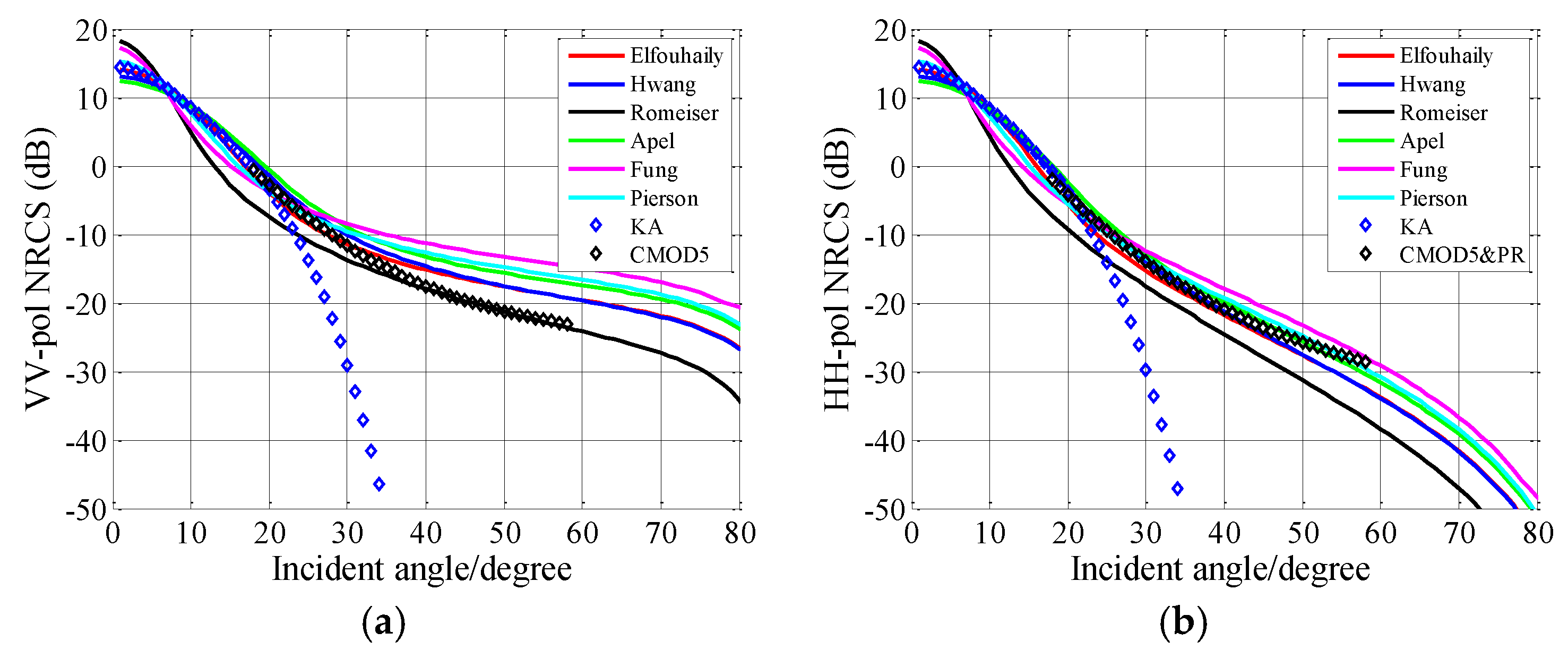
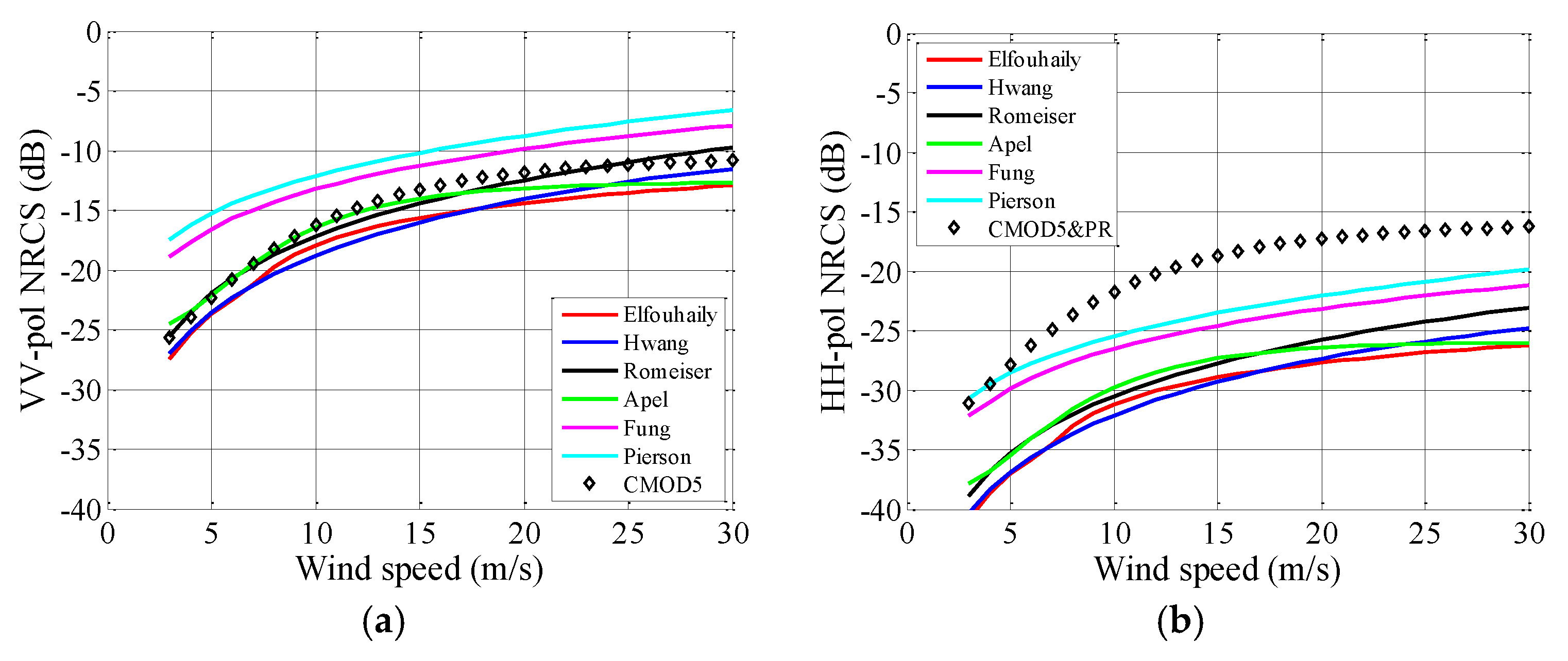
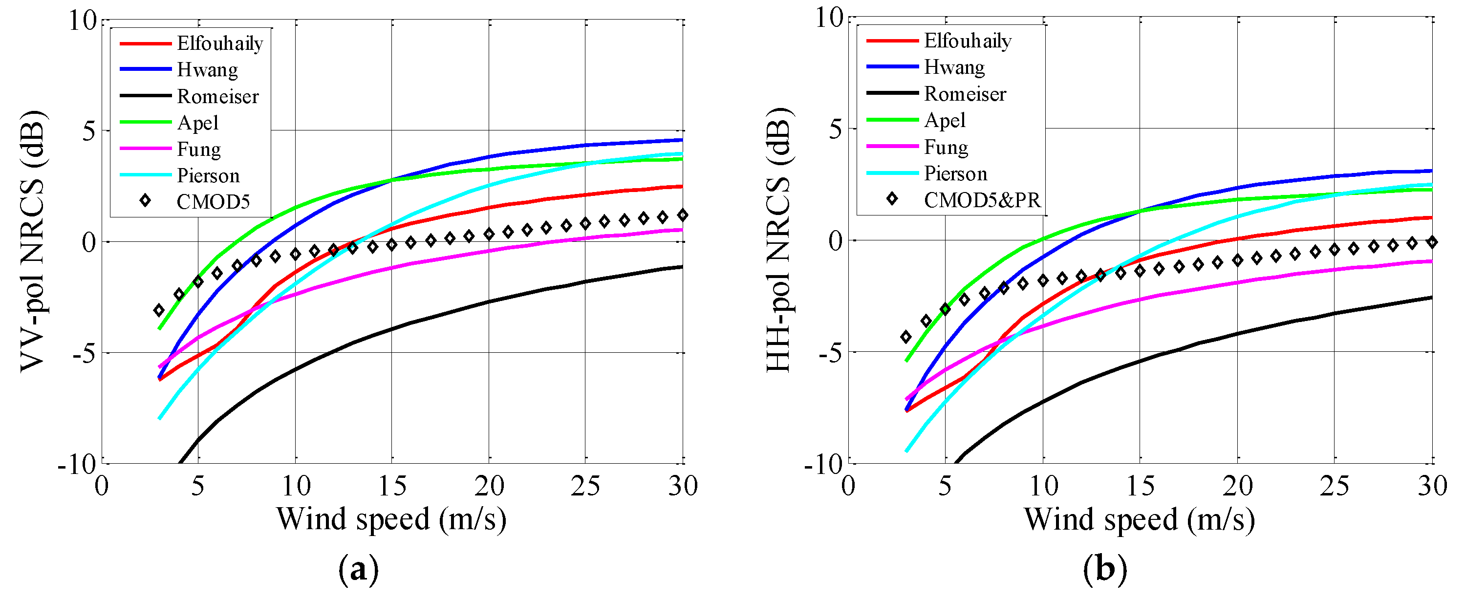
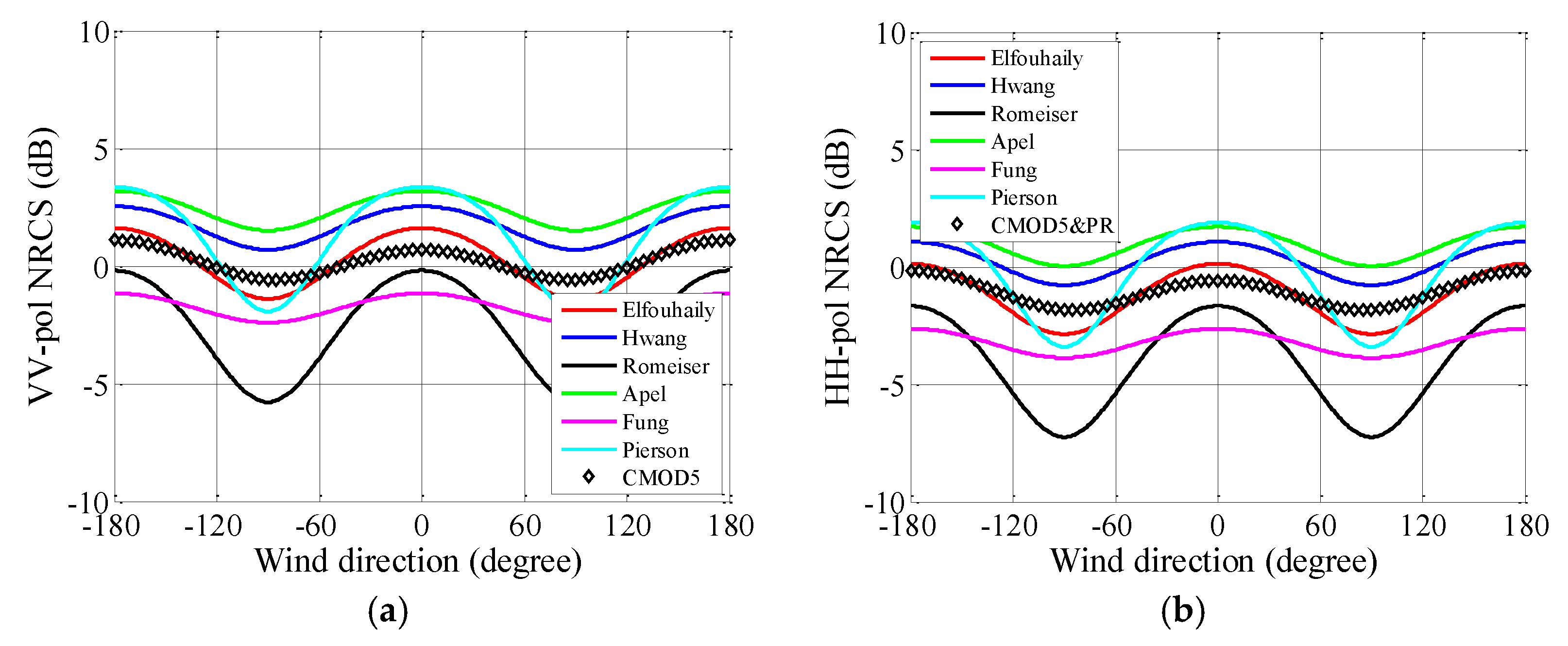
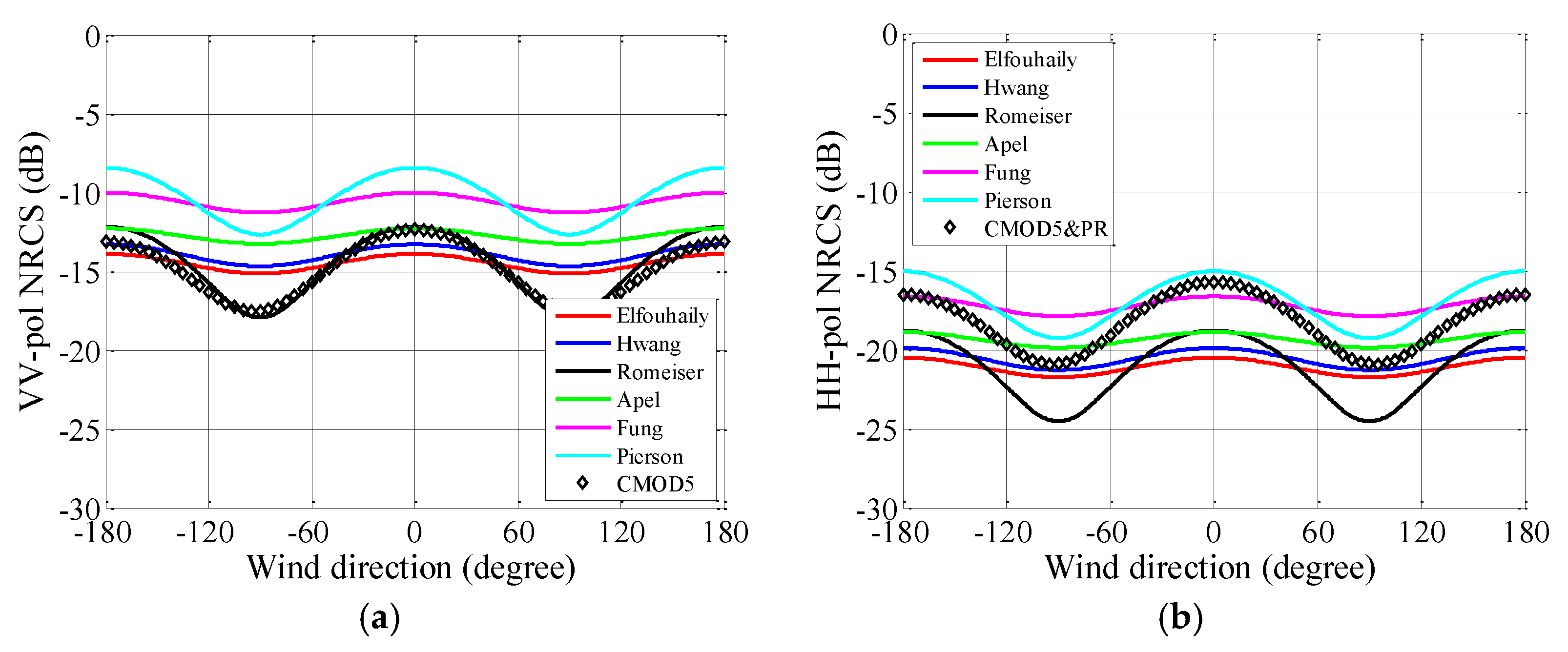
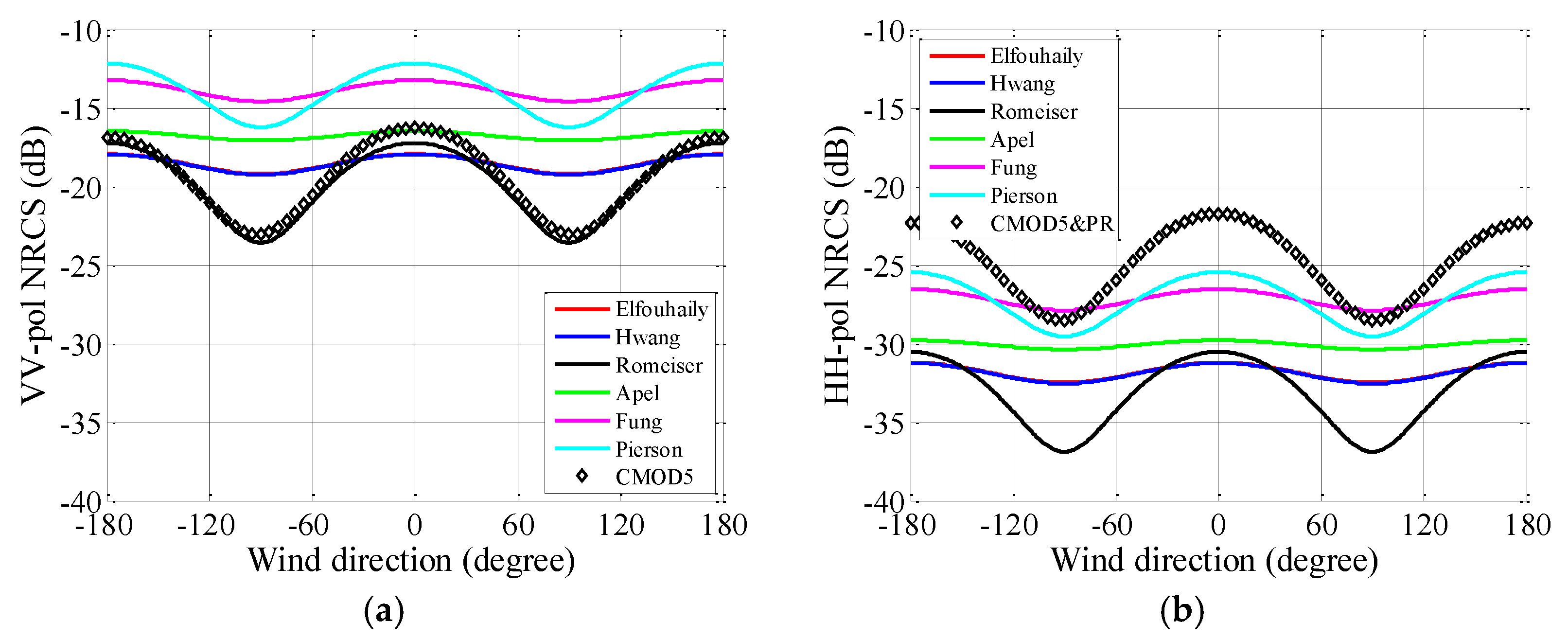
4.1.2. Evaluation with CMOD5

As most measured data are acquired under particular wind speed and wind direction, it is impossible to evaluate the accuracy of simulated results in all wind conditions. In the following, in order to evaluate the numerical simulations under different conditions, the simulated results are compared with the empirical model CMOD5. Simulations are made as functions of the incident angle, wind speed, wind direction, polarization state, and at a frequency equal to 5.3 GHz.

Incident Angle Variations

It has been reported that the KA (Kirchhoff Approximation) method could provide an accurate prediction in the specular region (θ_i = 0°~20°). In the following, numerical simulations are compared with KA for the specular region and CMOD5 for the moderate region. Here, only the case for U₁₀ = 10 m/s is presented and discussed in detail, and similar situations and conclusions can be obtained for U₁₀ = 5 m/s and U₁₀ = 15 m/s.

Figure 10 shows the scattering coefficients obtained as functions of incident angle for the upwind case. In Figure 10, both for HH and VV polarizations, the value of F- and P-spectra are larger than other curves, while the E-, H-, R-, and A-spectra exhibit similar results. This is because the spectral energies of the F-spectrum and P-spectrum are larger than other spectra (see Figure 1b, Figure 2b and Figure 3b). In the case of VV polarization, the NRCS calculated with the R-spectrum fits with the KA and CMOD5 better than other spectra, especially for the specular region (θ_i = 0°~20°). For the moderate region (θ_i = 20°~60°), the curves of the E-, H-, R-, and A-spectra exhibit similar results. As for Figure 10b, a similar phenomenon with VV polarization can be observed in the case of the HH polarization in the small incident angle range. Physically, the impacts caused by the polarization effect on the scattering coefficient are very small near the specular region. For the moderate region in the HH polarized channel, it seems that all the models underestimate the scattering coefficient. It is difficult to find a curve that matches well with the empirical model in all incident angle ranges.

For the upwind direction, we can see that the R-spectrum shows good agreement with CMOD5 and KA. However, according to Figure 6b, the difference between R-spectrum and Cox and Munk model cannot be neglected in crosswind direction. It is interesting to test these spectra in the crosswind direction. Figure 11 presents the scattering coefficients estimated in the crosswind direction. For the VV polarization, the R-spectrum cannot provide a good estimation as well as the upwind case when the incident angle is smaller than 30°. The E-spectrum and H-spectrum provide good estimations when the incident angle is smaller than 30°. For the HH polarization, it seems that the A- and P-spectra match well with empirical model for a moderate incident angle, and the H-spectrum matches well with the KA in the specular region.

In fact, as stated in Section 3, SSA-1 is an approximate method. That is to say, in our simulations, there may be some computational errors caused by SSA-1. Therefore, it does not mean that the R-spectrum performs better than other spectra in EM computations, it only illustrates that the R-spectrum provides a more accurate prediction with SSA-1 in the VV polarized channel for the upwind direction. Additionally, for the HH polarization, it is important to note that the inaccuracy may be, in part, introduced by the polarization ratio model.

Wind Speed and Direction Variations

For many ocean observations with microwave scatterometers, the basic principle relies on the scattering coefficient being strongly associated with wind speed and direction at the local sea surface. In the following part, the dependence of NRCS on wind speed and wind direction are studied. To show the wind speed and wind direction dependence in the C band, trend comparisons are made by plotting NRCS versus the wind speed and wind direction at moderate incident angles. Additionally, from the above analyses, we can know that the accuracies of the calculated scattering coefficients with different sea spectra are highly dependent on the incident angle. Here, three cases with different incident angles (18°, 40°, and 58°) are presented and discussed in detail.

In Figure 12, Figure 13 and Figure 14, the NRCSs are evaluated as functions of wind speed. The wind speed varies from 3 m/s to 30 m/s. As expected, the NRCSs increase with wind speed, except for the P-spectrum (see Figure 12a). According to Figure 12a, Figure 13a and Figure 14a, one can note that the increases of Efouhaily, Hwang, Romeiser, Apel, and CMOD5 curves induced by wind speed are similar. That is to say, for these spectra, the accuracies of calculated NRCSs are mainly associated with the incident angle and wind direction. For instance, the NRCS evaluated with the R-spectrum agrees well with CMOD5 in the upwind direction for incident angle ranges from 18° to 58° (see Figure 10a). Consequently, in all wind speed ranges, the curves of R-spectrum match well with CMOD5 (see Figure 12a, Figure 13a and Figure 14a). For the case of HH polarization, it appears that the calculated results seem to underestimate the NRCSs while the incident angles are set at 40° and 58°, which corresponding to Figure 10b. As previously stated, the underestimation of the HH polarization may be introduced by the PR model.

Apart from the upwind direction, we also investigated the crosswind direction. For the case of simplicity, only the comparisons for θ_i = 18° are presented in Figure 15. For VV polarization, as observed in Figure 11, the R-spectrum cannot provide a good estimation when the incident angle is smaller than 30°. Therefore, a large difference can be observed between the Romeiser curve and CMOD5 curve in Figure 15a. With respect to θ_i = 40° and θ_i = 58°, the influences of wind speed on Efouhaily, Hwang, Apel, and CMOD5 curves are similar.

Figure 16, Figure 17 and Figure 18 show the backscattering coefficients simulated under different wind directions for U₁₀ = 10 m/s. As illustrated in Figure 16, Figure 17 and Figure 18, all the curves have their maximum value in both upwind and downwind directions and their minimum at the crosswind direction. This behavior has been verified by many experimental measurements. Significant differences can be observed among the fluctuations (or the difference between peak and valley value) of different curves. These differences are caused by Δ(k) ratios plotted in Figure 4. As for the empirical model, it can be observed that the fluctuation along with wind direction increases with incident angle, while, for approximate results, the increases of fluctuations caused by the incident angle are smaller than CMOD5. It is not easy to find a curve that matches well with the empirical model in all cases. For VV polarization, the R-spectrum matches well with CMOD5 when the incident angle equals 40° and 58° in all wind directions.

Additionally, we have studied the cases of U₁₀ = 5 m/s and U₁₀ = 15 m/s. The fluctuations of CMOD5 under different wind directions are highly dependent on wind speed. None of the spectra could provide accurate predictions for all wind speed cases. For the case of U₁₀ = 5 m/s, the P-spectrum predicts the NRCS well for the HH polarization and θ_i = 58°. The R-spectrum predicts the NRCS well for the VV polarization and θ_i = 58°. For the case of U₁₀ = 15 m/s, the E-spectrum predicts the NRCS well, both for the HH and VV polarizations for θ_i = 18°. The P-spectrum predicts the NRCS well for the HH polarization and θ_i = 40°. The R-spectrum predicts the NRCS well for the VV polarization and θ_i = 40°.

4.2. Scattering from Sea Surface Observed in Bistatic Configuration

Compared with monostatic radar, bistatic radar is not used as widely. However, bistatic radar can offer certain advantages of spatial diversity and some level of covertness not offered by monostatic radar [20]. It is still necessary to study EM scattering from the sea surface in the bistatic configuration. Unfortunately, to our knowledge, there is no available experimental measurements or data in the published literature that can be used as references in our simulations.

As shown in Figure 19, in the configuration of the bistatic scattering problem, the transmitter radar wave $({\overrightarrow{E}}_i)$ evolves in the direction ${\overrightarrow{n}}_i$ in the plane $({\overrightarrow{h}}_i,{\overrightarrow{v}}_i)$. The scattered waves (${\overrightarrow{E}}_s$) in the receiver radar are in the direction ${\overrightarrow{n}}_s$ in the plane $({\overrightarrow{h}}_s,{\overrightarrow{v}}_s)$. The subscript i and s denote the incident and scattering wave, respectively. The incident and the scattered angles are ${\theta }_i$ and ${\theta }_s$, respectively. ${\varphi }_i$ and ${\varphi }_s$ are the incident and scattering azimuth angles, respectively [36].

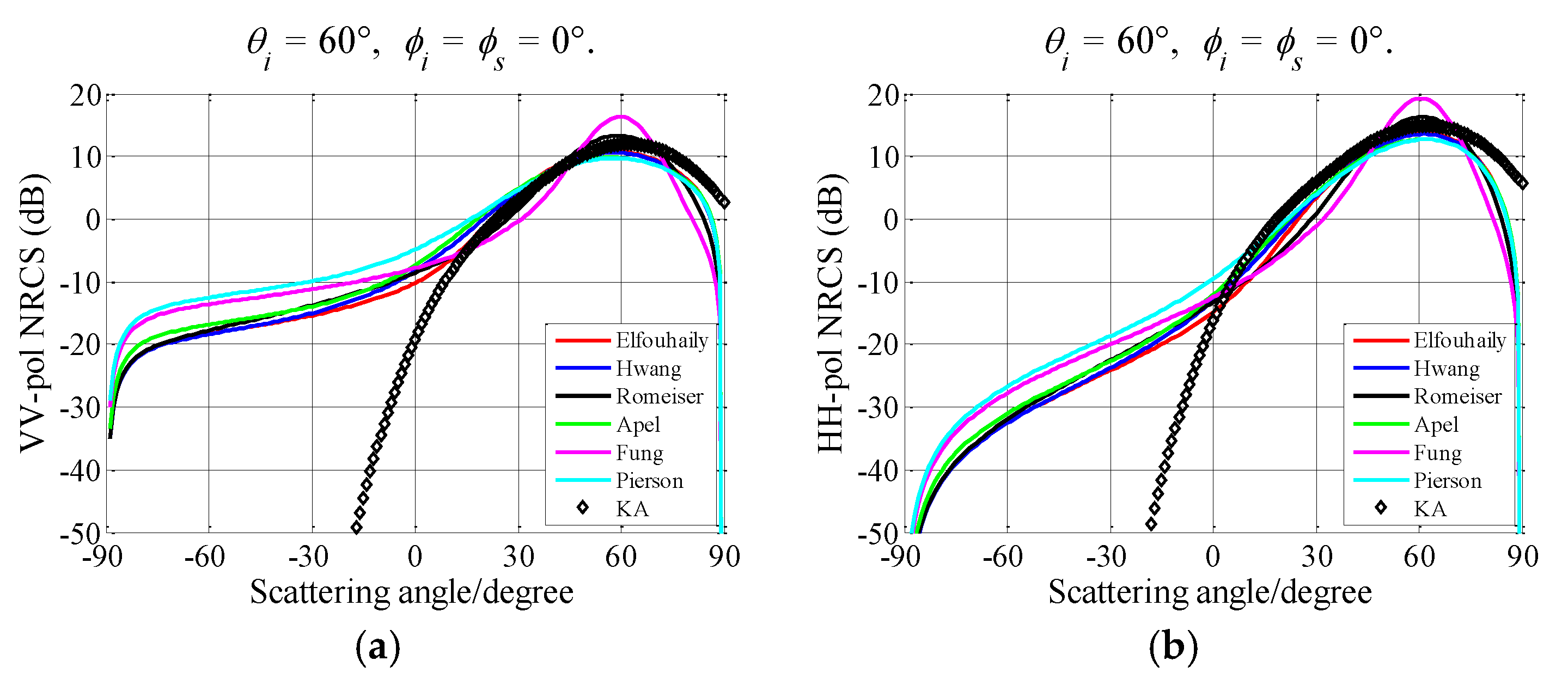
4.2.1. Scattering Angle Variation

Figure 20 exhibits the NRCSs estimated as functions of the scattering angle. The incident angle is set to 60°. The situation for the bistatic configuration is similar to the monostatic case. The NRCSs calculated with the F-spectrum and R-spectrum are higher than KA in specular region. The NRCSs calculated with F-spectrum and R-spectrum are higher while the scattering angle ranges from −90° to 0°.

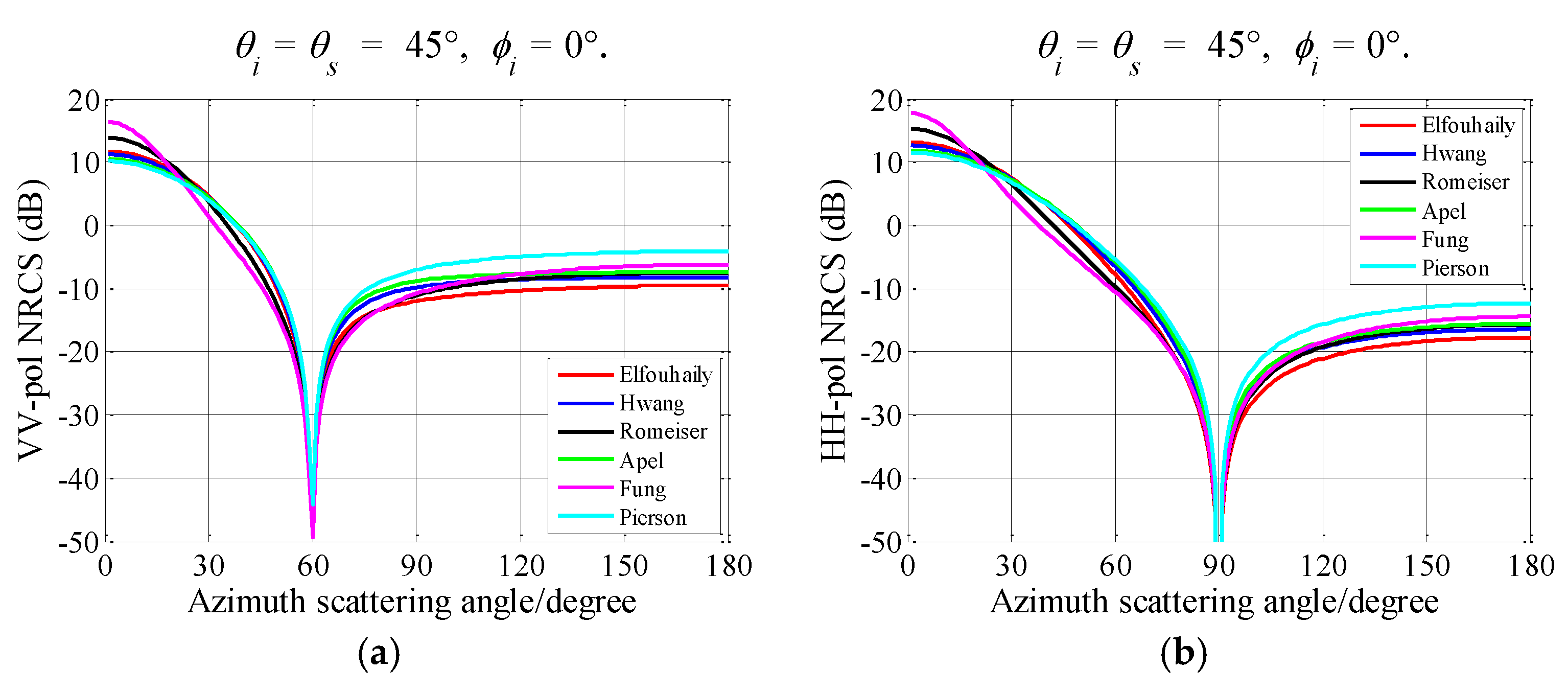
4.2.2. Scattering Azimuth Angle Variation

In Figure 21, the NRCSs versus the scattering azimuth angle curves are shown. The theoretical curves become flat with the scattering azimuth angle larger than 90° in the case of VV polarization and 120° in case of HH polarization. It is necessary to point out that the peaks in Figure 21 are not caused by physical reasons. They may be caused by the integral method during the computation. The locations of these peaks are associated with the incident angle.

5. Conclusions and Perspectives

In this paper, the numerical simulations of EM scattering using six different sea spectral models, including the commonly used E-spectrum and the newly-raised H-spectrum, are presented. A systematic comparison has been conducted in order to assess the performances of different models. Firstly, the spectral models proposed by different authors are compared and discussed from several points of view, including the omnidirectional parts, the angular spreading functions, the slope variances, and the autocorrelation functions. Several discrepancies between the different spectral models are noted. The analyses of the angular spreading functions and slope variances show that E- and H-spectra are in accordance with the measurements of Cox and Munk. Numerical simulations in monostatic and bistatic configurations are then performed. In the backscattering case, the results obtained with SSA-1 are compared with UAVSAR data in the L band and the empirical model CMOD5 in the C band. Compared with measured SAR data in the L band, both for VV and HH polarizations, the scattering coefficients evaluated using SSA-1 model are larger than the experimental data. However, the results obtained using E-spectrum are slightly better than the ones obtained using other spectra. Compared with CMOD5 in the C band, we find it difficult to accurately simulate the NRCS merely based on one spectral model in all wind speeds or wind directions. It is advised that different spectral models should be employed in different configurations to obtain accurate predictions. The following conclusions can be drawn from our analysis:

(1) For incident angle variation: The R-spectrum matches well with CMOD5 in the upwind direction. In the case of crosswind direction, for incident angle smaller than 30°, the E-spectrum and H-spectrum present better results. For incident angles larger than 30°, the R-spectrum presents better consistency with CMOD5.

(2) For wind speed variation: The influences of wind speed on the NRCSs computed using different sea spectra are similar.

(3) For wind direction variation: the fluctuations of CMOD5 under different wind directions are highly dependent on wind speed. None of the angular spreading functions could describe the direction of wave propagation exactly in all wind speed cases. However, in some cases, the NRCSs estimated with SSA-1 and sea spectrum agree well with CMOD5.

The simulations of NRCS in the monostatic configuration using different sea spectral models can be employed as a basis for inversion problems, such as retrieving the wind speed and direction from a radar image.

For the bistatic configurations, as there is not any available experimental data that can be used as a reliable reference, the scattering coefficients are only compared with KA as functions of the scattering angle. The differences between different curves in the bistatic configuration are similar to the monostatic case.

Additionally, it should be pointed out that, in this work, only the performances of different sea spectra with SSA-1 in the L and C bands have been investigated. In further works, more simulations and discussions will be conducted with other approximate methods, such as SPM, TSM, and SSA-2. In addition, and for different applications of interest, it would be useful to perform equivalent works in the X-band and Ku-band, comparing the contribution of asymptotic methods to the empirical model GMFs.

References

1. Ulaby, F.T.; Moore, R.K.; Fung, A.K. Chapter 12 Introduction to random surface scattering. In Microwave Remote Sensing Active and Passive-Volume II: Radar Remote Sensing and Surface Scattering and Emission Theory; Artech House: Norwood, UK, 1982; Volume 2, pp. 922–982. ISBN 0890061912. [Google Scholar]
2. Rice, S.O. Reflection of electromagnetic waves from slightly rough surfaces. Commun. Pure Appl. Math. 1951, 4, 351–378. [Google Scholar] [CrossRef]
3. Ogilvy, J.A.; Merklinger, H.M. Theory of wave scattering from random rough surfaces. J. Acoust. Soc. Am. 1991, 90, 3382. [Google Scholar] [CrossRef]
4. Voronovich, A.G. Small-slope approximation for electromagnetic wave scattering at a rough interface of two dielectric half-spaces. Wave Random Media 1994, 4, 337–367. [Google Scholar] [CrossRef]
5. Voronovich, A.G.; Zavorotny, V. Theoretical model for scattering of radar signals in Ku-and C-bands from a rough sea surface with breaking waves. Wave Random Media 2001, 11, 247–269. [Google Scholar] [CrossRef]
6. Voronovich, A.G. Chapter 6 “Nonclassical” Approaches to Wave Scattering at Rough Surfaces. In Wave Scattering from Rough Surfaces, 2nd ed.; Brekhovskikh, L.M., Felsen, L.B., Haus, H.A., Lotsch, H.K.Y., Eds.; Springer Science & Business Media: Berlin/Heidelberg, Germany, 1999; pp. 154–196. ISBN 3642599362. [Google Scholar]
7. Mouche, A.A.; Chapron, B.; Reul, N.; Hauser, D.; Quilfen, Y. Importance of the sea surface curvature to interpret the normalized radar cross section. J. Geophys. Res. Oceans 2007, 112, C10002. [Google Scholar] [CrossRef]
8. Pierson, W.J., Jr.; Moskowitz, L. A proposed spectral form for fully developed wind seas based on the similarity theory of S.A. Kitaigorodskii. J. Geophys. Res. 1964, 69, 5181–5190. [Google Scholar] [CrossRef]
9. Pierson, W.J., Jr.; Stacy, R.A. The Elevation, Slope, and Curvature Spectra of a Wind Roughened Sea Surface; NASA: Washington, DC, USA, 1973. [Google Scholar]
10. Bjerkaas, A.; Riedel, F. Proposed Model for the Elevation Spectrum of a Wind-Roughened Sea Surface; Johns Hopkins University Applied Physics Lab: Laurel, MD, USA, 1979. [Google Scholar] [CrossRef]
11. Fung, A.; Lee, K. A semi-empirical sea-spectrum model for scattering coefficient estimation. IEEE J. Ocean. Eng. 1982, 7, 166–176. [Google Scholar] [CrossRef]
12. Donelan, M.A.; Hamilton, J.; Hui, W.H. Directional spectra of wind-generated waves. Philos. Trans. R. Soc. Lond. A 1985, 315, 509–562. [Google Scholar] [CrossRef]
13. Apel, J.R. An improved model of the ocean surface wave vector spectrum and its effects on radar backscatter. J. Geophys. Res. Oceans 1994, 99, 16269–16291. [Google Scholar] [CrossRef]
14. Romeiser, R.; Alpers, W.; Wismann, V. An improved composite surface model for the radar backscattering cross section of the ocean surface: 1. Theory of the model and optimization/validation by scatterometer data. J. Geophys. Res. Oceans 1997, 102, 25237–25250. [Google Scholar] [CrossRef] [Green Version]
15. Elfouhaily, T.; Chapron, B.; Katsaros, K.; Vandemark, D. A unified directional spectrum for long and short wind-driven waves. J. Geophys. Res. Oceans 1997, 102, 15781–15796. [Google Scholar] [CrossRef] [Green Version]
16. Hwang, P.A. Observations of swell influence on ocean surface roughness. J. Geophys. Res. Oceans 2008, 113, C12024. [Google Scholar] [CrossRef]
17. Hwang, P.A. A note on the ocean surface roughness spectrum. J. Atmos. Ocean. Technol. 2011, 28, 436–443. [Google Scholar] [CrossRef]
18. Hwang, P.A.; Burrage, D.M.; Wang, D.W.; Wesson, J.C. Ocean surface roughness spectrum in high wind condition for microwave backscatter and emission computations. J. Atmos. Ocean. Technol. 2013, 30, 2168–2188. [Google Scholar] [CrossRef]
19. Hwang, P.A.; Fois, F. Surface roughness and breaking wave properties retrieved from polarimetric microwave radar backscattering. J. Geophys. Res. Oceans 2015, 120, 3640–3657. [Google Scholar] [CrossRef] [Green Version]
20. Awada, A.; Ayari, M.; Khenchaf, A.; Coatanhay, A. Bistatic scattering from an anisotropic sea surface: Numerical comparison between the first-order SSA and the TSM models. Wave Random Media 2006, 16, 383–394. [Google Scholar] [CrossRef]
21. Ayari, M.Y.; Khenchaf, A.; Coatanhay, A. Simulations of the bistatic scattering using two-scale model and the unified sea spectrum. J. Appl. Remote Sens. 2007, 1, 013532. [Google Scholar] [CrossRef]
22. Du, Y.; Yang, X.; Chen, K.-S.; Ma, W.; Li, Z. An improved spectrum model for sea surface radar backscattering at L-band. Remote Sens. 2017, 9, 776. [Google Scholar] [CrossRef]
23. Pugliese Carratelli, E.; Dentale, F.; Reale, F. Numerical PSEUDO—Random Simulation of SAR Sea and Wind Response. In Advances in SAR Oceanography from ENVISAT and ERS Missions, Proceedings of the SEASAR 2006 (ESA SP-613), Frascati, Italy, 23–26 January 2006; Lacoste, H., Ed.; ESA Publications Division: Noordwijk, The Netherlands, 2006. [Google Scholar]
24. Pugliese Carratelli, E.; Dentale, F.; Reale, F. Reconstruction of SAR Wave Image Effects through Pseudo Random Simulation. In Proceedings of the Envisat Symposium 2007 (ESA SP-636), Montreux, Switzerland, 23–27 April 2007; Lacoste, H., Ouwehand, L., Eds.; ESA Communication Production Office: Noordwijk, The Netherlands, 2007. [Google Scholar]
25. Bourlier, C.; Saillard, J.; Berginc, G. Intrinsic infrared radiation of the sea surface. J. Electromagn. Wave Appl. 2000, 14, 551–561. [Google Scholar] [CrossRef]
26. Cox, C.S.; Munk, W.H. Statistics of the sea surface derived from sun glitter. J. Mar. Res. 1954, 13, 198–227. [Google Scholar]
27. Zribi, M.; Gorrab, A.; Baghdadi, N. A new soil roughness parameter for the modelling of radar backscattering over bare soil. Remote Sens. Environ. 2014, 152, 62–73. [Google Scholar] [CrossRef] [Green Version]
28. Bourlier, C. Azimuthal harmonic coefficients of the microwave backscattering from a non-gaussian ocean surface with the first-order SSA model. IEEE Trans. Geosci. Remote Sens. 2004, 42, 2600–2611. [Google Scholar] [CrossRef]
29. Khenchaf, A. Bistatic scattering and depolarization by randomly rough surfaces: Application to the natural rough surfaces in X-band. Wave Random Media 2001, 11, 61–90. [Google Scholar] [CrossRef]
30. Hersbach, H.; Stoffelen, A.; de Haan, S. An improved C-band scatterometer ocean geophysical model function: CMOD5. J. Geophys. Res. Oceans 2007, 112, C03006. [Google Scholar] [CrossRef]
31. Yang, X.; Li, X.; Pichel, W.G.; Li, Z. Comparison of ocean surface winds from ENVISAT ASAR, MetOp ASCAT scatterometer, buoy measurements, and NOGAPS model. IEEE Trans. Geosci. Remote Sens. 2011, 49, 4743–4750. [Google Scholar] [CrossRef]
32. Zhang, B.; Perrie, W.; He, Y. Wind speed retrieval from Radarsat-2 quad-polarization images using a new polarization ratio model. J. Geophys. Res. Oceans 2011, 116, C08008. [Google Scholar] [CrossRef]
33. Verspeek, J.; Stoffelen, A.; Portabella, M.; Bonekamp, H.; Anderson, C.; Saldaña, J.F. Validation and calibration of ASCAT using CMOD5.n. IEEE Trans. Geosci. Remote Sens. 2010, 48, 386–395. [Google Scholar] [CrossRef]
34. Liu, G.; Yang, X.; Li, X.; Zhang, B.; Pichel, W.; Li, Z.; Zhou, X. A systematic comparison of the effect of polarization ratio models on sea surface wind retrieval from C-band synthetic aperture radar. IEEE J. Sel. Top. Appl. Earth Obs. Remote Sens. 2013, 6, 1100–1108. [Google Scholar] [CrossRef]
35. Li, H.; Perrie, W.; He, Y.; Wu, J.; Luo, X. Analysis of the polarimetric sar scattering properties of oil-covered waters. IEEE J. Sel. Top. Appl. Earth Obs. Remote Sens. 2015, 8, 3751–3759. [Google Scholar] [CrossRef]
36. Clarizia, M.P.; Gommenginger, C.; Di Bisceglie, M.; Galdi, C.; Srokosz, M.A. Simulation of L-band bistatic returns from the ocean surface: A facet approach with application to ocean GNSS reflectometry. IEEE Trans. Geosci. Remote Sens. 2012, 50, 960–971. [Google Scholar] [CrossRef]
Figure 1. Omnidirectional sea spectra for U10 = 5 m/s. (a) Full range. (b) Bragg scattering wavenumber range in the C band with an incident angle θi = 20°~60°.
Remotesensing 10 01084 g001
Figure 2. Omnidirectional sea spectra for U10 = 10 m/s. (a) Full range. (b) Bragg scattering wavenumber range in the C band with θi = 20°~60°.
Remotesensing 10 01084 g002
Figure 3. Omnidirectional sea spectra for U10 = 15 m/s. (a) Full range. (b) Bragg scattering wavenumber range in the C band with θi = 20°~60°.
Remotesensing 10 01084 g003
Figure 4. Δ(k) ratios given by different authors: (a) U10 = 5 m/s; (b) U10 = 10 m/s; and (c) U10 = 15 m/s.
Remotesensing 10 01084 g004
Figure 5. Angular spreading functions given by different authors, k = 135 rad/m: (a) U10 = 5 m/s; (b) U10 = 10 m/s; and (c) U10 = 15 m/s.
Remotesensing 10 01084 g005
Figure 6. RMS slopes inferred from spectral and models Cox and Munk model. (a) In the upwind direction. (b) In the crosswind direction.
Remotesensing 10 01084 g006
Figure 7. Omnidirectional normalized autocorrelation functions. (a) U10 = 5 m/s; (b) U10 = 10 m/s; and (c) U10 = 15 m/s.
Remotesensing 10 01084 g007
Figure 8. UAVSAR data. (a) Case (a); and (b) Case (b).
Remotesensing 10 01084 g008
Figure 9. Comparisons between SSA-1 and UAVSAR data. (a) VV polarization. (b) HH polarization.
Remotesensing 10 01084 g009
Figure 10. NRCSs estimated in relationships to incident angle. U10 = 10 m/s, ϕ = 0 ° . (a) VV polarization. (b) HH polarization.
Remotesensing 10 01084 g010
Figure 11. NRCSs estimated in relationships to incident angle. U10 = 10 m/s, ϕ = 90 ° . (a) VV polarization. (b) HH polarization.
Remotesensing 10 01084 g011
Figure 12. NRCSs estimated in relationship to the wind speed. θi = 18°, ϕ = 0 ° . (a) VV polarization. (b) HH polarization.
Remotesensing 10 01084 g012
Figure 13. NRCSs estimated in relationship to the wind speed. θi = 40°, ϕ = 0 ° . (a) VV polarization. (b) HH polarization.
Remotesensing 10 01084 g013
Figure 14. NRCSs estimated in relationship to the wind speed. θi = 58°, ϕ = 0 ° . (a) VV polarization. (b) HH polarization.
Remotesensing 10 01084 g014
Figure 15. NRCSs estimated in relationship to the wind speed. θi = 18°, ϕ = 90 ° . (a) VV polarization. (b) HH polarization.
Remotesensing 10 01084 g015
Figure 16. NRCSs estimated in relationship to the wind direction. U10 = 10 m/s, θi = 18°. (a) VV polarization. (b) HH polarization.
Remotesensing 10 01084 g016
Figure 17. NRCSs estimated in relationship to the wind direction. U10 = 10 m/s, θi = 40°. (a) VV polarization. (b) HH polarization.
Remotesensing 10 01084 g017
Figure 18. NRCSs estimated in relationship to the wind direction. U10 = 10 m/s, θi = 58°. (a) VV polarization. (b) HH polarization.
Remotesensing 10 01084 g018
Figure 19. Geometrical configuration for the bistatic scattering from sea surface.
Remotesensing 10 01084 g019
Figure 20. NRCSs estimated based on different sea spectra as a function of the scattering angle. U10 = 10 m/s, upwind. (a) VV polarization; (b) HH polarization.
Remotesensing 10 01084 g020
Figure 21. NRCSs estimated based on the different sea spectra as functions of the scattering azimuth angle. U10 = 10 m/s. (a) VV polarization; and (b) HH polarization.
Remotesensing 10 01084 g021