Article

Modified Multi-Mode Target Tracker for High-Frequency Surface Wave Radar

1
Institute of Electronic and Engineering Technology, Harbin Institute of Technology, Harbin 150001, China
2
Key Laboratory of Marine Environmental Monitoring and Information Processing, Ministry of Industry and Information Technology, Harbin 150001, China
*
Author to whom correspondence should be addressed.
Remote Sens. 2018, 10(7), 1061; https://doi.org/10.3390/rs10071061
Submission received: 29 May 2018 / Revised: 2 July 2018 / Accepted: 3 July 2018 / Published: 4 July 2018
(This article belongs to the Special Issue Radar Remote Sensing of Oceans and Coastal Areas)

Abstract

:
In high-frequency surface wave radar (HFSWR), part of the radiation signal inevitably propagates upward and illuminates the target through the ionosphere due to the poor controllability of the antenna’s vertical pattern. As a result, a target may have several echoes from different propagation modes, which affect target detection and tracking and is usually unmanageable in existing HFSWR systems. Without the information of the elevation angle, it is difficult to distinguish the propagation mode of measurements during the target detection phase. This paper makes the first attempt to propose a multi-mode target tracker for HFSWR to solve this problem during the target tracking phase. The multipath probability data association (MPDA) tracker is capable of exploiting multipath target signatures of discrete propagation modes and has been widely used. Based on this, we construct a modified multi-mode probability data association tracker for HFSWR to suppress false tracks caused by multiple propagation modes. Numerical simulations demonstrate that this novel tracker can effectively and accurately track the target from the measurements under multiple propagation modes in HFSWR. The processing results of the actual data collected in Weihai, China indicate that this tracker is of great significance for practical applications.

1. Introduction

High-frequency surface wave radar (HFSWR) usually consists of a one-dimensional line array with weak control of the vertical pattern. Therefore, energy cannot be strictly radiated along the sea surface and partially radiates upwards and impinges on the ionosphere. In some cases, the incident skywave energy may be reflected or scattered by the target or ionosphere and return to the receiver [1]. In fact, HF radar signals propagate through the ionosphere in three ways: the first is near-vertical reflection; the second is to emit a wave at an angle less than vertical, reflected by the ocean or the target, and then back along the same path or sea surface; the third is back-scattering phenomenon caused by the irregularities and the fluctuations of the ionosphere [2]. Traditionally, in HFSWR, ionospheric echo is generally considered as clutter, and there have been many studies on ionospheric clutter suppression [2,3]. However, in the second scenario, ionospheric echo may carry the information of the target (such as a plane, island, or vessel).
It is worth noting that the presence of the ionospheric echo of the target can extend the detection range of the HFSWR, which has not been considered or analyzed in the previous HFSWR systems. This paper proposes a novel tracker to solve the problem of false tracks in long-range detection of HFSWR, making it possible to expand the surveillance area of HFSWR. This is very favorable for marine environmental monitoring, and it can be directly applied to existing HFSWR systems without adding additional equipment.
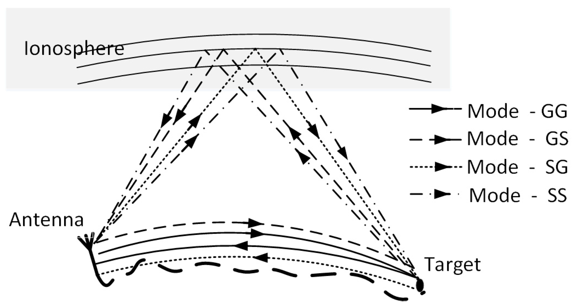
However, the existence of ionospheric echo results in several echoes corresponding to one target (the phenomenon of multiple propagation modes) in HFSWR. Irrespective of ionospheric stratification, there are four propagation modes, as shown in Figure 1: emit and receive the wave through the ground wave path—GG, emit/receive the wave through the ground wave path and receive/emit the wave from the ionosphere—GS/SG, emit the wave to the ionosphere and receive the wave from the ionosphere—SS [4].
The phenomenon of multiple propagation modes results in the following problems:
(a)
One target may have several measurements and one measurement may correspond to many targets, which may cause false detections;
(b)
The actual ground range calculation formula for each propagation modes are different, therefore, misjudgment of the measurement’s propagation mode will lead to a false estimation of the target’s true position; and
(c)
One target may form multiple tracks.
Note that, multipath phenomenon caused by ionospheric stratification also exists. In addition, multiple propagation modes’ phenomenon also brings some advantages. The skywave propagation mode propagates farther than the groundwave propagation mode because its attenuation is smaller and decays slower than the ground attenuation. Hence, if we analyze the echoes of multiple propagation modes together, the detection range of HFSWR can be expanded. However, we need to solve those problems caused by multiple propagation modes’ phenomenon at first. In addition, since the skywave propagation mode echo may exceed the unambiguity range of the existing HFSWR, this paper extends the unambiguity detection range of HFSWR through a range ambiguity resolution method to observe the echoes of all propagation modes more effectively.
The key of the above problems lies in how to judge the propagation mode of the measurements. The direct method is to obtain the echo’s elevation angle which, however, is difficult for HFSWR, due to one-dimensional line array is deployed there. Some researches on two-dimensional arrays has been proposed, for example, Ref. [5] uses L-shaped arrays to suppress ionospheric interference and Ref. [6] uses 4 × 4 square planar arrays to mitigate ionospheric clutter. However, it is still difficult to solve the multi-mode problems in the target detection phase, because mode SG (GS) cannot be distinguished with mode GG (SS) through the elevation angle. Therefore, in this paper, we consider to solve the multi-mode problems when tracking targets for a one-dimensional array HFSWR system.
Target tracking in HFSWR has been extensively studied, and it mainly consists of various filters to describe the target movement properly, such as the Kalman filter [7], deferred decision filter [8], extended Kalman filter [9], and unscented Kalman filter [10], etc. To enhance the tracking performance in clutter background, many data association algorithms are employed to HFSWR, such as near neighbor data association [11], probabilistic data association (PDA) [12] and joint probabilistic data association (JPDA) [13]. There are also some knowledge-based tracking algorithms for reducing the probability of the track breaking [14]. However, all those tracking method cannot solve the multi-mode problem and will result in false tracks.
Multipath phenomenon of over the horizon radar (OTHR) caused by ionosphere stratification also forms false tracks, and there are two common types of methods for tracking. The first type is to establish a target dynamical model based on the radar coordinate system, and applying a data association tracking algorithm to achieve tracking under the radar coordinate system. After tracking, one target may form multiple tracks. Then, the track fusion algorithm is applied to find which tracks correspond to the same target and calculate the real target track. The data association tracking algorithm includes Viterbi data association (VDA) [15], probabilistic data association (PDA) [16] and probabilistic multi-hypothesis tracking (PMHT) [17], etc. The track fusion algorithm includes a dynamic weighted fusion algorithm [18], a sequential track-to-track fusion algorithm [19], etc. The second type establishes the target dynamical model under the geographic coordinate system and completes the data association in the radar coordinate system. This type of method can obtain the real target track directly (only one track for one target). The corresponding data association algorithm includes multipath data association (MPDA) [20], multipath Viterbi data association (MVDA) [21], Markov chain Monte Carlo (MCMC) [22], and expectation maximization data association (EMDA) [23], etc. The tracking accuracy of MCMC and EMDA is high, but their computation is heavy. MPDA uses Markov chain to characterize the probability transfer of target state; MVDA uses the dynamic programming optimization framework to merge or delete data association hypotheses, which is sub-optimal. Those algorithms have both advantages and disadvantages.
The essential difference between the two types of methods is that the target dynamic model is based on different coordinate systems. The first type is based on the radar coordinate system, while the second type is under the geographic coordinate system. In addition, the first type of method does not need the prior knowledge of the ionosphere, and can work stably without relying on coordinate transformation. However, it will form many tracks correspond to one target, which needs track fusion to obtain the real target track. Therefore, this type of method has a higher track loss rate when the echoes of some modes are not detected, while the second type of method requires coordinate transformation and ionosphere status information, which will introduce errors and degrade tracking stability, but the track loss rate is lower. Certain modes’ echoes may not happen because of the path attenuation and the instability of the ionosphere, which will be analyzed in Section 2. Therefore, we choose the second type of method. Since this paper is the first attempt to propose the multi-mode target tracking for HFSWR, we chose to modify the MPDA tracker that has been widely used.
In Section 2, we analyze the multiple propagation modes’ phenomenon in HFSWR, and study the coverage of each propagation mode by analyzing path attenuation. Then, we show the processing results of the actual data collected in Weihai, China to illustrate the existence of multiple propagation modes’ phenomenon (false tracks). In Section 3, we construct a modified multi-mode probability data association tracker. MPDA establishes a target dynamical model and measurement model in the geographic coordinate and the radar coordinate, respectively. Thus, firstly, we show the target dynamical model and measurement model. The target dynamical model uses a linear discrete-time model described by range, velocity, azimuth, and azimuth rate. The measurement model is constructed through the geometrical relationship between target ground range and each propagation mode’s path length and it consists of path length, azimuth, and velocity. Obviously, the measurement model is nonlinear, so the Jacobian of the coordinate transformation is also needed. Moreover, a one-point initiation algorithm proposed in [20] is modified to apply to HFSWR. In Section 4, the simulation results show that the modified multi-mode probability data association tracker can suppress false tracks and track the real target correctly. Moreover, the multi-mode target tracker is successfully applied to the actual data and it found a trajectory, which should be a plane flying to Hohhot, China.

2. Multiple Propagation Modes’ Phenomenon Analysis

Considering that both the groundwave path and the skywave path exist in HFSWR, there should be four propagation modes irrespective of ionospheric stratification, labeled as GG, GS, SG, and SS, as shown in Figure 1. However, the plasma distribution of the ionosphere varies with height, time, solar activity, latitude and longitude, etc. According to the plasma distribution, the ionosphere is usually divided into three layers, the E-layer, the Es-layer, and the F-layer, which may be separated into the F1-layer and F2-layer [
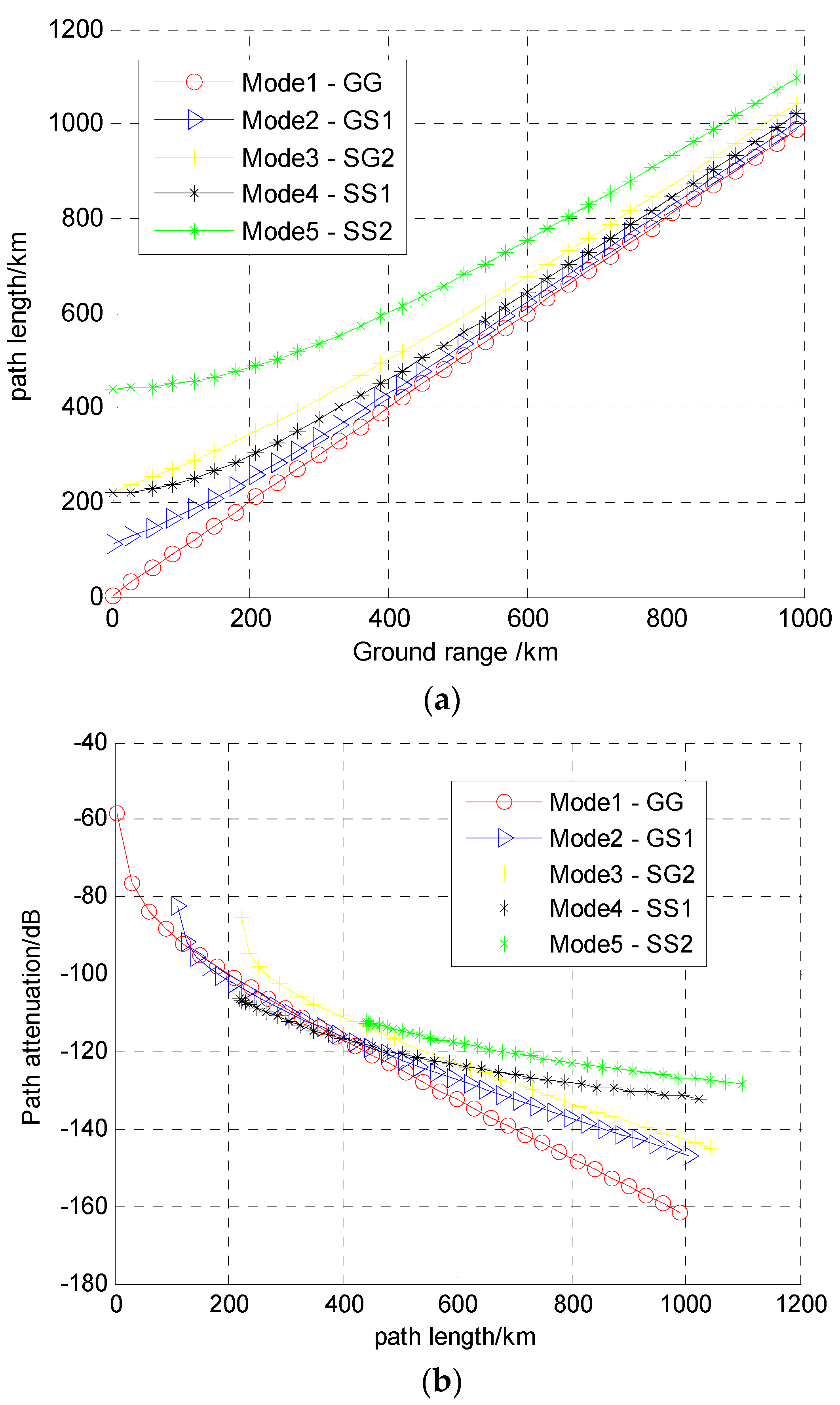
24]. The layer from which the wave is reflected is uncertain and is related to the frequency, angle of incidence, and site, etc. Therefore, considering the complexities of the ionosphere, there will be quite a large number of propagation modes. In order to reduce the complexity of the tracking algorithm when taking the ionospheric characteristics into account, we only analyze these five propagation modes in this paper—Mode 1-GG, Mode 2-GS1 (ionospheric height is h 1 ), Mode 3-SG2 (ionospheric height is h 2 ), Mode 4-SS1 (ionospheric height is h 1 ), and Mode 5-SS2 (ionospheric height is h 2 ).
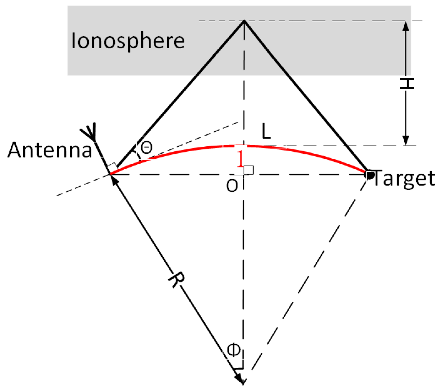
Then, we calculate the attenuation of each mode through their corresponding groundwave attenuation and skywave attenuation. Here, groundwave attenuation is calculated by the groundwave-propagation program GRWAVE developed by Rotheram [25], and skywave attenuation is calculated according to the empirical formula proposed by CCIR (Consultative Committee of International Radio) [26]. Moreover, the path length of each mode is calculated through the geometric relationship, as shown in Figure 2 and its calculation formula is the same as the measurement model that will be given in Section 3.
Figure 3a shows that the path length (the length calculated through the echo’s delay time) of each of five propagation modes is a function of ground range (target’s ground range). Here, the ionospheric heights are h 1 = 110   km and h 2 = 220   km , and the electromagnetic frequency is 5 MHz. Figure 3b shows the path attenuation (the electric field level) in five propagation modes changing with the path length. It can be seen that there is one propagation mode within 200 km, four modes in the range of 200 km to 400 km, and five modes over 400 km. In addition, as the distance increases, the path attenuation is so large that the target cannot be detected. In this case, the number of propagation modes may be less than the theoretical value. The multipath range is also related to electromagnetic frequency and the ionospheric state, which will not be analyzed in detail in this paper.
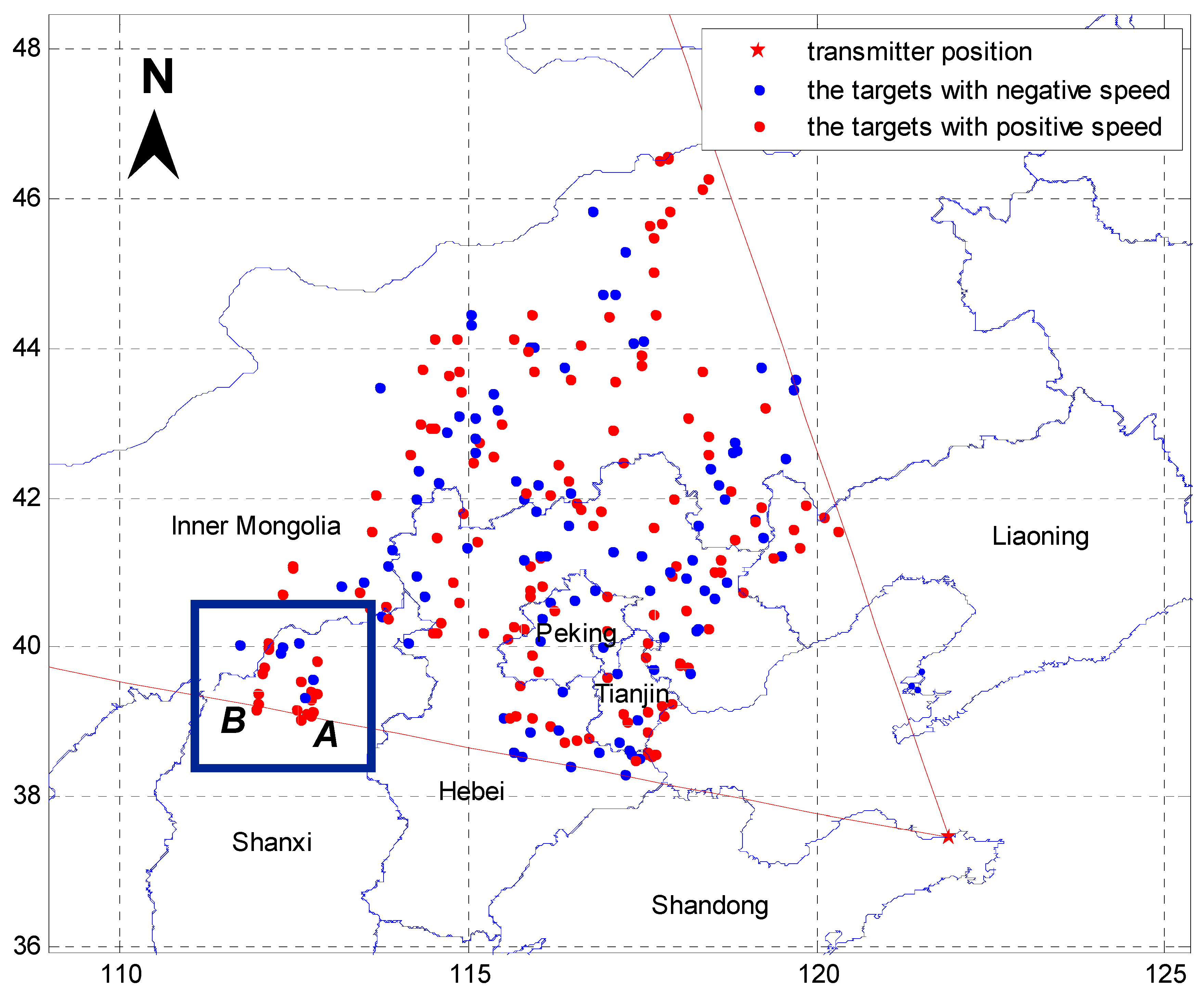
Next, the actual data collected in Weihai, China is processed to illustrate the existence of the phenomenon of multiple propagation modes’. The processing result is shown in Figure 4, where red dots represent the detection targets with positive speed (the target is approaching the radar), and blue dots represent the detection targets with negative speed (the target is moving away from the radar). As the illuminated area is inland, a large amount of clutter affects the detection performance. Within 900–1100 km, we determine two suspected tracks, represented by green (track A) and yellow (track B) squares, respectively. The measured values of the two suspected tracks are shown in Table 1 and Table 2.
Firstly, we calculate the ground distance of every measurement of the two tracks with two different ionospheric height. We assume the ionospheric heights for tracks A and B are 140 km and 200 km, respectively, then we calculate the ground distance, as shown in the third column of Table 1 and Table 2. Then, we calculate the absolute value of the difference between the two tracks’ parameters at each moment, as shown in Table 3. Using the accuracy of the measurements as a criterion. The accuracy of the distance measurements is 1 km, the accuracy of velocity is 0.6 m/s, and the accuracy of azimuth is five degrees. Since the ionospheric height is not accurate, the accuracy of the distance will increase, set to 5 km. We find that the differences between the two tracks’ ground distance, velocity, and azimuth are smaller than 5 km, 0.6 m/s, and five degrees, respectively, and, according to our criteria, the two tracks are corresponding to the same target. Therefore, there are multiple tracks (false tracks) for one target, i.e., the phenomenon of multiple propagation modes in HFSWR.
After the above analysis, we know that the two tracks should come from one target. The echoes of modes GG/SG1/GS2 of this target have not been detected because path attenuation of the target at about 900 km in these three modes is very high. However, this is also a case of the phenomenon of multiple propagation modes in HSFWR.

3. Modified Multi-Mode PDA Tracker for HFSWR

To suppress false tracks, this section constructs a modified multi-mode PDA tracker, which consists of target dynamical model, measurement model, track initiation, event probabilities and state estimator. For simplicity, we assume a non-maneuvering and constant-velocity aircraft tracking in an ideal ionospheric state.

3.1. Target Dynamical Model

The target state at time k is described in ground coordinates through ground range L ( k ) (length of the red line 1 in Figure 2), ground range rate L ˙ ( k ) , azimuth θ ( k ) (angle with the center of illuminating aperture angle), azimuth rate θ ˙ ( k ) . Therefore, the target status at time k is written as:
x ( k ) = [ L ( k ) L ˙ ( k ) θ ( k ) θ ˙ ( k ) ] ,
We assume that the target moves along a straight line with a certain deviation which can be expressed as an additive noise term v ( k ) . Then, the equation of target status can be given by a recursion formula:
x ( k + 1 ) = Fx ( k ) + v ( k ) ,
where the matrix F is given by:
F = [ 1 T 0 0 0 1 0 0 0 0 1 T 0 0 0 1 ] ,
T is the revisit time, v ( k ) is a white Gaussian sequence with zero-mean and covariance Q ( k ) which is calculated according to [22]:
Q ( k ) = ( T 3 δ p 2 / 3 T 2 δ p 2 / 2 0 0 T 2 δ p 2 / 2 T δ p 2 0 0 0 0 T 3 δ b 2 / 3 T 2 δ b 2 / 2 0 0 T 2 δ b 2 / 2 T δ b 2 ) ,
where δ p 2 and δ b 2 are the noise variance of range and bearing filter, respectively.

3.2. Measurement Model

The radar measurement consists of path length R s (delay time of echo), velocity R r , and azimuth A z (angle with the center of illuminating aperture angle). Hence, the measurement vector at time k is defined as follows:
y ( k ) = [ R s ( k ) R r ( k ) A z ( k ) ] ,
The target measurement is a non-linear function of target status x ( t ) and associated with propagation mode. Assuming that there are N k propagation modes, their measurement equation is expressed as:
y m ( k ) = H m ( x ( k ) ) + w m ( k ) , m = 1 , , N k ,
where m is the index of propagation mode, y m ( k ) is the measurement vector of the m th mode, w m ( t ) is the measurement noise term of the m th mode with zero-mean and covariance R m ( k ) . Assuming v ( k ) and w ( k ) is unrelated. R m ( k ) can be obtained as:
R m ( k ) = cov ( w m ( k ) ) = ( δ R 2 0 0 0 δ D 2 0 0 0 δ A 2 ) ,
where δ R 2 , δ D 2 , and δ A 2 are the error variances of range, velocity, and azimuth, respectively.
The measurements are obtained under radar coordinates, H m ( ) in measurement equation is the mapping from ground coordinates X to radar coordinates Y. From the geometric relations shown in Figure 2, the coordinate transformation formula from X to Y of five propagation modes 1-GG, 2-GS1, 3-SG2, 4-SS1, and 5-SS2 (Table 4) are expressed as follows
{ R s m = a ( m ) L + b ( m ) K ( m ) R r m = a ( m ) L ˙ + b ( m ) S ( m ) A z m = θ , m = 1 , , 5 ,
a = [ 1 1 / 2 1 / 2 0 0 ] ,
b = [ 0 1 / 2 1 / 2 1 1 ] ,
h = [ 0 h 1 h 2 h 1 h 2 ] ,
K = 2 ( μ sin ( L 2 μ ) ) 2 + ( h + μ ( 1 cos ( L 2 μ ) ) ) 2 ,
S = 2 ( h + μ ) R g sin ( L 2 μ ) L ˙ ,
where μ is the earth radius, h contains two different ionospheric height— h 1 and h 2 .
As a result, H m ( ) in the measurement equation is as follows:
H m ( x ) = [ a ( m ) L + b ( m ) K ( m ) a ( m ) L ˙ + b ( m ) S ( m ) θ ] , m = 1 , , 5 ,
The Jacobian of transformation from ground coordinates to radar coordinates is defined as follows:
J m = y x = [ a ( m ) + b ( m ) A ( m ) 0 0 0 b ( m ) B ( m ) a ( m ) + b ( m ) A ( m ) 0 0 0 0 1 0 ] , m = 1 , , 5 ,
A = 2 ( h + μ ) R s sin ( L 2 μ ) ,
B = 2 ( h + μ ) L ˙ R s 2 ( cos ( L 2 μ ) R s 2 μ sin ( L 2 μ ) R r L ˙ ) ,

3.3. Initiation

In this paper, we apply a one-point initiation algorithm proposed by [20]. This algorithm forms the initial state estimates for all propagation modes, which can prevent certain modes from being missed. For each valuable measurement y ( k ) = [ R s R r A z ] in scan k, this algorithm forms an initial state estimate x ^ m ( 0 | 0 ) = [ L L ˙ θ θ ˙ ] of every propagation mode m (GG, GS1, SG2, SS1, SS2) using the appropriate ionospheric height h, i.e., mapping measurements from Y to X. The initial covariance P ( 0 | 0 ) is assigned based on the known measurement noise variances R . The formula for mapping measurements from Y to X is:
G G : { L = R s L ˙ = R r θ = A z θ ˙ 0 ,
G S 1 / S G 2 : { L = 2 h ( R s μ + R g 2 μ 2 μ h ( h 2 R s 2 ) ) L ˙ = R r 1 2 + h + μ R s sin ( L 2 μ ) θ = A z θ ˙ 0 ,
S S 1 / 2 : { L = 2 μ cos 1 ( h 2 + 2 μ 2 + 2 μ h R s 2 / 4 2 μ 2 + 2 μ h ) L ˙ = R r R s 2 ( h + μ ) sin ( L 2 μ ) θ = A z θ ˙ 0 ,
where h = h 1 for mode GS1 and SS1, h = h 2 for mode SG2 and SS2. Moreover, h 1 and h 2 are assigned according to the predicted value of the ionospheric height.
The mapping from Y- R s to X- L of mode GS1/SG2 needs to solve the transcendental equation. For its calculation, here we substitute the cosine with the first two terms of its Taylor’s expansion. Figure 5 shows the transformation errors of modes GS1/SG2 mapping from Y- R s to X- L . It can be seen that the ground range error increases rapidly with ground range, the error within the distance of interest (0 to about 1000 km) is acceptable for track initiation.

3.4. Event Probabilities

Tracking a single target determines the minimum mean-square-error estimator (MMSE) x ^ ( k | k ) of the state x ( k ) based on the multi-mode measurement process.
The PDA tracker needs to exhaust all possible associations of valid measurements with propagation modes. In order to reduce the number of valid detections, a validation gate (or region) for each mode is needed at each scan k, as shown in Figure 6 (G1 and G2). In heavy clutter, we define a validation gate for each target state estimate, “a validation region or ‘gate’ in the measurement space in which we expect to see a detection from the target at the next dwell. In this way, many detections that are statistically distant from the expected target location are eliminated from the processing. Detections falling within the validation region are referred to as validated or gated measurements for that target” [22]. For every validation gate G m ( k ) of mode m, we can obtain the validated measurement sets { y 1 ( k ) , , y M k ( k ) } by judging whether the measurement y in the k-th scan satisfies:
G m ( k ) { y 3 : [ y y ^ m ( k + 1 | k ) ] ( S m ( k + 1 ) ) 1 [ y y ^ m ( k + 1 | k ) ] < γ m } , m = 1 , , N k ,
where N k is the number of propagation modes, the scalar constant γ m is determined by the validation gate probability P G m ( k ) in the k-th scan based on hypothesis testing of χ 2 ( n ) , n is the measurement vector dimension (equal to three in this paper). y ^ m ( k + 1 | k ) and S m ( k + 1 ) are the predicted measurement and corresponding covariance for mode m respectively, which can be calculated by the following formulas:
x ^ ( k + 1 | k ) = F x ^ ( k | k ) ,
P ( k + 1 | k ) = FP ( k | k ) F + Q ( k ) ,
y ^ m ( k + 1 | k ) = H m ( x ^ ( k + 1 | k ) ) , m = 1 , , N k ,
S m ( k + 1 ) = J m P ( k + 1 | k ) J m ( k + 1 ) + R m ( k ) , m = 1 , , N k ,
where x ^ ( k + 1 | k ) is the predicted state that obtained by one-point initiation algorithm, P ( k + 1 | k ) is the prediction covariance, and J m ( k + 1 ) is the Jacobian of the measurement equation H m ( x ) evaluated at the current predicted state x ^ ( k + 1 | k ) for mode m.
Then, we need to exhaust all possible associations. Let θ i , m j ( t ) denote the i-th possible association hypothesis for the j - th ( j = 1 , , M k ) validated measurements when the number of active modes at time k is m { 0 , , min ( M k , N k ) } . It satisfies:
θ i , m j = { t h e a s s o c i a t e d m o d e , i f t a r g e t 0 , i f c l u t t e r ,
Let r k ( m ) denote the number of association hypotheses at time k when the active modes’ number is m.
For example, if there are three valid measurements { y 1 ( k ) , y 2 ( k ) , y 3 ( k ) } in two validation gates { G 1 ( k ) , G 2 ( k ) } as shown in Figure 6, there are nine possible association hypotheses: when m = 0 , r ( 0 ) = 1 , { θ 1 , 0 1 = 0 , θ 1 , 0 2 = 0 , θ 1 , 0 3 = 0 } ; when m = 1 , r ( 0 ) = 4 , { θ 1 , 1 1 = 1 , θ 1 , 1 2 = 0 , θ 1 , 1 3 = 0 } , { θ 2 , 1 1 = 0 , θ 2 , 1 2 = 1 , θ 2 , 1 3 = 0 } , { θ 3 , 1 1 = 0 , θ 3 , 1 2 = 2 , θ 3 , 1 3 = 0 } , { θ 4 , 1 1 = 0 , θ 4 , 1 2 = 0 , θ 4 , 1 3 = 2 } ; when m = 2 , r ( 0 ) = 5 , { θ 1 , 2 1 = 1 , θ 1 , 2 2 = 1 , θ 1 , 2 3 = 0 } , { θ 2 , 2 1 = 1 , θ 2 , 2 2 = 2 θ 2 , 2 3 = 0 } , { θ 3 , 2 1 = 1 , θ 3 , 2 2 = 0 , θ 3 , 2 3 = 2 } , { θ 4 , 2 1 = 0 , θ 4 , 2 2 = 1 , θ 4 , 2 3 = 2 } ; { θ 5 , 2 1 = 0 , θ 5 , 2 2 = 2 , θ 5 , 2 3 = 2 } .
Next, for active modes m = 0 , 1 , , N k and feasible association hypotheses i = 1 , , r k ( n ) at time k, we compute the event probabilities β ¯ ( k ) , β 0 ( k ) and { β i , n ( k ) } .
β ¯ ( k ) represents the probability of the event that the target does not exist and all detections in the validation gate are clutter. β 0 ( k ) represents the probability of the event that the target exists and is observable by all modes, but all measurements in the validation gate are clutter. { β i , m ( k ) } represents the probability of the event that the target exists and is observable and the measurements fall in the validation gate of mode m = 1 , , N k [20].
Denote Pr ( E k | Y k 1 ) and Pr ( E ¯ k | Y k 1 ) to represent the target existence possibility and inexistence possibility, respectively. The probabilities are governed by a homogeneous Markov chain with known transition matrix M:
M = ( Pr ( E k | E k 1 ) Pr ( E ¯ k | E k 1 ) Pr ( E k | E ¯ k 1 ) Pr ( E ¯ k | E ¯ k 1 ) ) ,
The propagation Markov chain is:
[ Pr ( E k | Y k 1 ) Pr ( E ¯ k | Y k 1 ) ] = M [ Pr ( E k 1 | Y k 1 ) Pr ( E ¯ k 1 | Y k 1 ) ] ,
We choose the Poisson model to describe the clutter. Hence, the probability of n clutter measurements in the validation region G ( k ) is:
g c ( n ) = ( λ V G ( k ) ) n e λ V G ( k ) n ! , n = 0 , 1 , 2 , ,
where, λ is the density of detections, V G is the volumes of validation region G ( k ) .
Then, the event probabilities are:
β ¯ ( k ) = δ k 1 Pr ( E ¯ k | Y k 1 ) λ M k M k ! exp { λ V G ( k ) } ,
β 0 ( k ) = δ k 1 Pr ( E k | Y k 1 ) ( 1 P D P G ) N k λ M k M k ! exp { λ V G ( k ) } ,
β i , m ( k ) = δ k 1 Pr ( E k | Y k 1 ) ( P D ) m ( 1 P D P G ) N k m 1 r k ( m ) × j { j : θ i , m j 0 } ( 2 π ) n y / 2 ( det S q ( k ) ) 1 / 2 exp { 1 2 d j q } × { 1 c m = 0 exp { λ V G ( k ) } λ M k m ( M k m ) ! c m > 0 m = 1 , , min { M k , N k } , i = 1 , , r k ( m ) ,
d j q = ( y j ( k ) y ^ q ( k | k 1 ) ) S q ( k ) 1 ( y j ( k ) y ^ q ( k | k 1 ) ) ,
q = θ i , m j ( k ) 1 ,
where δ k is a normalization factor at time k, n y is the dimension of the measurement vector, P D is the probability of detection, and P G is the validation gate probability.

3.5. State Estimator

For every possible association hypothesis, the conditional state estimates x ^ i , m ( k + 1 | k + 1 ) and covariance P i , m ( k + 1 | k + 1 ) , i = 1 , , r k ( m ) , m = 1 , , min { M k , N k } are calculated according to the following formulas:
x ^ i , m ( k | k ) x ^ ( k | k 1 ) + j { j : θ i , m j 0 } l { l : θ i , m l 0 } P ( k | k 1 ) × J q j j l ( k ) { y j ( K ) y ^ q l ( k | k 1 ) } ,
P i , m ( k | k ) P ( k | k 1 ) j { j : θ i , m j 0 } l { l : θ i , m l 0 } P ( k | k 1 ) × J q j j l ( k ) J q l ( k ) P ( k | k 1 ) ,
Next, we form the iterative update equation for the state estimate as expressed in Equation (37) and the state estimation error covariance as expressed in Equation (38):
x ^ ( k | k ) = { β ¯ ( k ) + β 0 ( k ) } x ^ ( k | k 1 ) + n = 1 min ( M k , N k ) i = 1 r k ( n ) β i , n ( k ) x ^ i , n ( k | k ) ,
P ( k | k ) = β 0 ( k ) P ( k | k 1 ) + β ¯ ( k ) P ¯ ( k ) + { β ¯ ( k ) + β 0 ( k ) } x ^ ( k | k 1 ) x ^ ( k | k 1 ) x ( k | k ) x ( k | k ) + n = 1 min ( M k , N k ) i = 1 r k ( n ) β i , n ( k ) { P i , n ( k | k ) + x ^ i , n ( k | k ) x ^ i , n ( k | k ) ,
We repeat the above steps of Section 3.4 and Section 3.5 using the update state estimate x ^ ( k | k ) and the state estimation error covariance P ( k | k ) .

4. Numerical Simulation and Actual Data Processing

In this section, we give the simulation results of the modified multi-mode PDA tracker and then apply the tracker to process the actual data collected in Weihai, China. Table 5 lists the simulation parameters of target state model and measurement model.
For the validation gate, the gate probability at the k-th scan P G ( k ) is set to 0.95, same for each propagation mode. According to the hypothesis testing of χ 2 ( 3 ) , the scalar constant γ should be 7.8. The clutter density is assigned 0.002.
Then, we assume that the probability of target detection P D is the same for all propagation mode. Markov transition matrix M is:
M = [ 0.75 0.25 0.05 0.95 ] ,
When the probability of target detection P D is equal to 0.4, the tracking result is shown in Figure 7a and the tracking error is given in Figure 7b. The false tracks are suppressed and the target state is estimated correctly.
The actual data collected in Weihai, China has been analyzed in Section 2. Since the detection number is enormous and the suspected target tracks’ locations are known, we just apply the modified multi-mode PDA tracker to the measurements around the suspected two tracks as shown in Figure 8. According to the previous analysis, the two suspected tracks belong to the same target, that is, the multiple propagation modes’ phenomenon. If we use the traditional tracking method, two tracks appear. The tracking result of the proposed tracker is shown in Figure 9 and the arrows indicate the direction of target movement. We can determine that the tracking results are basically consistent with the analysis in Section 2. The tracking result has only one track without false tracks. Therefore, the processing result proves that the modified multi-mode PDA tracker is significant for HFSWR to suppress false tracks caused by the phenomenon of multiple propagation modes.

5. Conclusions

The ionospheric echo of the targets in the HFSWR can be used to detect the targets at further distances, which have not received sufficient attention in the past. However, this will lead to the problem of multi-mode transmission, which is the main issue of this paper. We propose the multi-mode target tracking to solve the multiple propagation modes’ problem causes by the existence of ionospheric echo in HFSWR. The multiple propagation modes’ problem caused several measurements for one target, which will affect target detection and tracking. This problem can be solved by the modified multi-mode PDA tracker. The simulation results show that the tracker can track targets without false tracks. In addition, the tracker is applied to actual data collected in Weihai, China, and the processing result indicates the tracker is significant for HFSWR to solve problem of the multiple propagation modes.

Author Contributions

Conceptualization, M.Z. and Q.Y.; Methodology, M.Z.; Software, M.Z.; Validation, M.Z., X.Z. and Q.Y.; Formal Analysis, M.Z.; Investigation, X.Z. and Q.Y.; Resources, Q.Y.; Data Curation, Q.Y.; Writing-Original Draft Preparation, M.Z.; Writing-Review & Editing, M.Z., X.Z. and Q.Y.; Visualization, M.Z.; Supervision, X.Z..; Project Administration, Q.Y.; Funding Acquisition, Q.Y.

Funding

This research was funded by [the National Natural Science Foundations of China] grant number [61171182 and 61701140].

Acknowledgments

Thanks to the Key Laboratory of Marine Environmental Monitoring and Information Processing, Harbin Institute of Technology, China for data support. Due to laboratory regulations, data cannot be disclosed for the time being. If the readers request a copy, please contact Yang Qiang whose email address is yq@hit.edu.cn.

Conflicts of Interest

The authors declare no conflict of interest.

References

  1. Thayaparan, T.; MacDougall, J. Evaluation of ionospheric sporadic-E clutter in an arctic environment for the assessment of high-frequency surface-wave radar surveillance. IEEE Trans. Geosci. Remote Sens. 2005, 33, 1180–1188. [Google Scholar] [CrossRef]
  2. Wu, M.; Wen, B.Y.; Zhou, H. Ionospheric Clutter Suppression in HF Surface Wave Radar. J. Electromagn. Wave Appl. 2009, 23, 1265–1272. [Google Scholar] [CrossRef]
  3. Chen, Z.; Xie, F.; Zhao, C.; He, C. An Orthogonal Projection Algorithm to Suppress Interference in High-Frequency Surface Wave Radar. Remote Sens. 2018, 10, 403. [Google Scholar] [CrossRef]
  4. Zhao, M.; Yang, Q. A new way of estimating ionospheric virtual height based on island multipath echoes in HFSWR. In Proceedings of the Radar Conference, Seattle, WA, USA, 8–12 May 2017; pp. 576–580. [Google Scholar]
  5. Xianrong, W.; Hengyu, K.; Biyang, W. Adaptive ionospheric clutter suppression based on subarrays in monostatic HF surface wave radar. IEE Proc.-Radar Sonar Navig. 2005, 152, 89–96. [Google Scholar] [CrossRef]
  6. Tian, W.; Li, G.; Xu, R. Ionosphere Interference Suppression for HFSWR using L-Shape Array. In Proceedings of the 2010 2nd International Conference on Signal Processing System, Dalian, China, 5–7 July 2010; pp. V1-484–V1-488. [Google Scholar]
  7. Riddolls, R.J.; Adve, R.S. Two-dimensional adaptive processing for ionospheric clutter mitigation in High Frequency Surface Wave Radar. In Proceedings of the Radar Conference, Barcelona, Spain, 26–29 April 2009; pp. 1–4. [Google Scholar]
  8. Ponsford, A.M.; Wang, J. A review of high frequency surface wave radar for detection and tracking of ships. Turk. J. Electr. Eng. Comput. Sci. 2010, 18, 409–428. [Google Scholar]
  9. Dzvonkovskaya, A.; Gurgel, K.W.; Rohling, H.; Thomas, S. HF radar WERA application for ship detection and tracking. Eur. J. Navig. 2009, 7, 18–25. [Google Scholar]
  10. Huang, X.J.; Wen, B.Y.; Ding, F. Ship detection and tracking using multi-frequency HFSWR. IEICE Electron. Express 2010, 7, 410–415. [Google Scholar] [CrossRef] [Green Version]
  11. Braca, P.; Grasso, R.; Vespe, M.; Maresca, S.; Horstmann, J. Application of the JPDA-UKF to HFSW radars for maritime situational awareness. In Proceedings of the IEEE International Conference on Information Fusion, Singapore, 9–12 July 2012; pp. 2585–2592. [Google Scholar]
  12. Chan, H.C. Iceberg Detection and Tracking Using High Frequency Surface Wave Radar; Defense Research Establishment Ottawa: Ottawa, ON, Canada, 1997. [Google Scholar]
  13. Bar-Shalom, Y.; Daum, F.; Huang, J. The probabilistic data association filter. IEEE Control Syst. Mag. 2009, 29, 82–100. [Google Scholar] [CrossRef]
  14. Chen, B.; Tugnait, J.K. Tracking of multiple maneuvering targets in clutter using IMM/JPDA filtering and fixed-lag smoothing. Automatica 2001, 37, 239–249. [Google Scholar] [CrossRef]
  15. Vivone, G.; Braca, P.; Horstmann, J. Konwledge-based multi-target ship tracking for HF surface wave radar systems. IEEE Trans. Geosci. Remote Sens. 2015, 53, 3931–3949. [Google Scholar] [CrossRef]
  16. Scala, B.L.; Pulford, G. Viterbi Data Association Tracking for Over-the-Horizon Radar. In Proceedings of the International Radar Symposium, Munich, Germany, 15–17 September 1998; pp. 1155–1164. [Google Scholar]
  17. Kirubarajan, T.; Bar-Shalom, Y. Probabilistic data association techniques for target tracking in clutter. Proc. IEEE 2004, 92, 536–557. [Google Scholar] [CrossRef]
  18. Zhang, Y.; Ran, J. Dynamic weighted track fusion algorithm based on track comparability degree. In Proceedings of the IEEE International Conference on Information Theory and Information Security, Beijing, China, 17–19 December 2010; pp. 710–713. [Google Scholar]
  19. Tian, X.; Barshalom, Y. Sequential track-to-track fusion algorithm: Exact solution and approximate implementation. In Proceedings of SPIE; The International Society for Optical Engineering: Washington, DC, USA, 2008; Volume 6969, p. 696910. [Google Scholar]
  20. Streit, R.L.; Luginbuhl, T.E. Probabilistic Multi-Hypothesis Tracking; Naval Underwater Systems Center: Newport, RI, USA, 1995. [Google Scholar]
  21. Pulford, G.W.; Evans, R.J. A multipath data association tracker for over-the-horizon radar. IEEE Trans. Aerosp. Electron. Syst. 1998, 34, 1165–1183. [Google Scholar] [CrossRef]
  22. Pulford, G.; Scala, B.L. Over-The-Horizon Radar Tracking Using the Viterbi Algorithm Second Report to HFRD; Cooperative Research Center for Sensor Signal and Information Processing (CSSIP), University of Melbourne: Melbourne, Australia, 1995. [Google Scholar]
  23. Bergman, N.; Doucet, A. Markov chain Monte Carlo data association for target tracking. IEEE Trans. Autom. Control 2009, 54, 481–497. [Google Scholar]
  24. Zhang, X.; Yao, D.; Yang, Q.; Dong, Y.; Deng, W. Knowledge-Based Generalized Side-Lobe Canceller for Ionospheric Clutter Suppression in HFSWR. Remote Sens. 2018, 10, 104. [Google Scholar] [CrossRef]
  25. Rotheram, S. Ground-wave propagation Part 2: Theory for medium and long distances and reference propagation curves. IEE Proc. 1981, 128, 285–295. [Google Scholar] [CrossRef]
  26. Consultative Committee of International Radio (CCIR). Second CCIR Computer-Based Interim Method for Estimating Sky-Wave Field Strength and Transmission Loss at Frequencies between 2 and 30 MHz; CCIR Recommendation 252-2; CCIR: Geneva, Switzerland, 1992. [Google Scholar]
Figure 1. Four possible transmission paths leave out the ionospheric stratification in HFSWR.
Remotesensing 10 01061 g001
Figure 2. Mathematical model considering the Earth’s curvature.
Remotesensing 10 01061 g002
Figure 3. (a) Five modes’ path lengths as a function of the ground range; and (b) the path attenuation in five propagation modes changing with the path length.
Remotesensing 10 01061 g003
Figure 4. Actual data processing results (red dots represent the detection targets with positive speed (the target is approaching the radar), blue dots represent the detection targets with negative speed (the target is moving away from the radar), and the area between the red lines is the radar’s surveillance area).
Remotesensing 10 01061 g004
Figure 5. Transformation error of modes GS/SG mapping from Y- R s to X- L .
Remotesensing 10 01061 g005
Figure 6. Illustrative gating scenario in azimuth-range-Doppler space with two propagation modes and three validated measurements.
Remotesensing 10 01061 g006
Figure 7. Simulation result when detection probability is 0.4: (a) estimate target trajectory compared to true target trajectory; and (b) estimate target state error.
Remotesensing 10 01061 g007
Figure 8. All measurements around the suspected tracks.
Remotesensing 10 01061 g008
Figure 9. Tracking result of actual data collected in Weihai, China.
Remotesensing 10 01061 g009
Table 1. Tracking parameters of Track A.
TimePath Length/kmGround Distance/kmVelocity m/sAzimuth/Degrees
10:57:5697493433.8−27
10:58:0397393334.1−27
10:58:1097193033.9−28
10:58:1797193133.6−28
10:58:2497193033.3−27
10:58:3196992833.3−27
Table 2. Tracking parameters of Track B.
TimePath Length/kmGround Distance/kmVelocity m/sAzimuth/Degrees
10:57:49101393233.6−29
10:57:56101393233.2−28
10:58:03101092934.4−27
10:58:10101393233.8−25
Table 3. The absolute value of the difference between two tracks’ tracking parameters.
TimeGround Distance/kmVelocity m/sAzimuth/Degrees
10:57:49---
10:57:5620.61
10:58:0340.30
10:58:1010.13
10:58:17---
10:58:24---
10:58:31---
Table 4. Index of propagation modes.
Index12345
ModeGGGSSGSSSS
h - h 1 h 2 h 1 h 2
Table 5. Simulation parameters.
LabelParameterValue
TRevisit time10 (s)
LTotal number of iterations50
x ( 0 | 0 ) The initial state of target100 km, 0.15 km/s,
5 deg, 0.001 deg/s
δ p Range noise standard deviation 10−6 (km)
δ d Bearing filter noise standard deviation5 × 10−5 (deg)
δ R 2 Range error variance0.0025 (km2)
δ D 2 Velocity error variance0.0001 ((m/s)2)
δ A 2 Azimuth error variance0.04 (deg2)

