1. Introduction
Interactions between processes such as wind, surface water and tide are dominant factors driving the movement of water in coastal regions. Good understanding of surface currents is necessary for operations such as search and rescue and oil spill movement, especially short-term real time forecasting information of surface currents with high accuracy.
Numerical models and observation platforms based on remote sensing technologies are conventional tools to study characteristics of coastal surface currents and provide useful information. However, each approach has its own limits. Numerical models that mathematically describe dynamic processes are often used to produce forecasts of surface currents. Difficulties in the definition of initial and boundary conditions, grid structure on horizontal and vertical planes and simplification of parameters inevitably result in model errors that may be significant. Oceanic observation tools such as satellites, radars and Acoustic Doppler Current Profiles (ADCP) are powerful means of monitoring near real-time oceanic currents over large spatial domains; however, these tools cannot implicitly provide forecasting states of surface currents.
To obtain high accuracy forecasting states of oceanic parameters such as surface velocities by making the best use of available observations, Kalman filters, variational data assimilation and particle filters have been used as to improve modeling forecast accuracy [
1,
2,
3,
4]. However, the establishment of a data assimilation system is a major task as it usually requires significant computational cost such as the calculation of model background errors in Kalman filters and the adjoint model in four-dimensional variational (4D-VAR) data assimilation systems [
5]. Other forecasting techniques include Decision Tree (DT), Fuzzy Inference System (FIS) and Artificial Neural Networks (ANN) using observations of coastal parameters [
6,
7,
8]. Soft computing approaches can be generally categorized into one of two types based on the learning algorithm: (i) supervised soft computing approaches such as ANN and DT; and (ii) unsupervised soft computing approaches such as Principal Component Analysis (PCA), clustering algorithms and self-organizing maps (SOM). A supervised soft computing model is developed herein via training processes that not only generate forecasts but also correct forecasts when they deviate significantly from the target outputs in the training dataset. Training procedures are run until forecasts reach a desired level of accuracy on the training dataset. In unsupervised soft computing approaches, models are built up by reducing data structures, such as dimensionality. System reduction of redundancy via a mathematical process or organization of data by similarity may be used for unsupervised soft computing approaches [
9,
10,
11]. For example, PCA is a statistical unsupervised procedure that uses an orthogonal transformation to convert a dataset of possibly correlated variables into a set of values of linearly uncorrelated principal components [
12].
Since relationships between input and output variables are directly correlated in soft computing approaches, the development process is less time-consuming and faster than conventional fluid dynamics models. Because the authors focused on predicting coastal surface velocities in terms of observed surface currents in this research, a supervised soft computing approach, ANN, was adopted in this research to develop an accurate short-term forecasting system. Several researchers have successfully applied ANN algorithms in various fields to produce forecasts of diverse parameters: Chen and Lin [
13] applied ANN to predict mobile station location; Aydogan et al. [
14] employed ANN to predict current velocity in the Strait of Istanbul using ADCP data; Partal et al. [
15] developed daily precipitation forecasts model with ANN; Makarynskyy et al. [
16] applied ANN to predict waves at the west coast of Portugal; Yang and Xia [
17] developed data-driven forecasting model of mining subsidence based on field measurements and artificial neural networks; and Erzin and Cetin [
18] applied ANN to predict the critical factor of safety of homogeneous finite slopes. Zabada and Shahrour [
19] analyzed heating expenses in a large social housing stock in the north of France using ANN model. All the studies showed that ANN algorithms are powerful and efficient for extracting internal relationships among input, and can generate high accuracy forecasting states in a wide range of application. Additionally, a wide range of ocean, coastal and environmental issues have already been solved using ANNs to approximate nonlinear processes without any knowledge of interrelations among the variables [
20,
21,
22,
23]. In this research, the authors focused on using high frequency radar (HFR) data to develop ANN forecast models through examining historical observation as input variables and optimizing topology of input variables to extend practical forecasting period for ocean surface currents. The advantages of using ANN algorithms over other techniques are:
- (1)
ANN is a highly nonlinear algorithm, capable of describing nonlinear dynamic processes such as surface currents generated by tide and winds of interest here.
- (2)
ANN algorithms provide the capability of dealing with datasets in the absence of knowledge about system physics.
- (3)
ANN techniques use meshless computational approaches to directly correlate relationships between input variables and output variables through recognizing historic patterns [
24].
- (4)
ANN models require much less computational cost than conventional fluid dynamics models.
- (5)
Once an ANN model is established and validated, it can be used for other periods of interest as long as appropriate input datasets are available.
- (6)
ANN models are capable of dealing with finite number of discontinuities [
25].
- (7)
ANN models are suitable for parallel processing if long term or fast outputs are required [
25].
The primary objective of this research was to assess the potential for applying ANN algorithms to develop high-accuracy forecasts of surface currents using HFR data recorded at Galway Bay. Products of short-term high accuracy surface currents can be used for gap filling in radar vector fields, search and rescue and oil spill response. Surface currents can also be useful to determine the origin of phytoplankton communities including potentially harmful species [
26]. Moreover, HFR data can be used to derive wave characteristics [
27,
28]. Hourly surface currents were measured by a Coastal Ocean Dynamic Application Radar (CODAR) system; surface currents in Galway Bay are mainly driven by tide and wind forces [
3,
29,
30]. Thus, tide and wind parameters are considered as the main input variables to develop ANN models. Mahjoobi and Adeli Mosabbeb [
31] used current data and those belonging to the previous hours as inputs to predict significant wave heights using a soft computing approach (Support Vector Machine (SVM)), satisfactory forecasts were obtained. Malekmohamadi et al. [
32] also used hourly wind speeds at previous time steps to predict wave heights with four different soft computing approaches—ANN, SVM, Adaptive Neuro-Fuzzy Inference System (ANFIS) and Bayesian Networks (BN). Malekmohamadi et al. [
32] found that the ANN, ANFIS and SVM approaches can provide acceptable predictions for wave heights, while the BN’s results are unreliable. Londhe et al. [
33] used previous values of data to develop ANN models to predict forecasting errors of significant wave heights via coupling with a numerical model. Results indicate that numerical model forecasts were improved considerably by adopting an ANN approach. Gauci et al. [
34] also used past measurements of HFR data and satellite wind observations to fill gaps of HFR data with ANN technique. Karimi et al. [
35] used previous sea level values to establish ANN and ANFIS models. Karimi et al. [
35] found that ANN and ANFIS models gave similar forecasts and outperformed auto-regression moving average models (ARMA) for all the prediction intervals. Frolov et al. [
36] developed a statistical model for predicting surface currents based on historical HFR observations and forecasted winds. Frolov et al. [
36] found that the minimal length of the HF-radar data required to train an accurate statistical model was between one and two years, depending on the accuracy desired. To establish an efficient short-term high accuracy forecasting system using ANN technique, the general method proposed by Mahjoobi and Adeli Mosabbeb [
31] was applied in this research by taking previous observations of surface current components as input variables. The reason for including historical current data is that the variation of surface flow fields is consistent in time and space, and the development of surface flows at the present time step is significantly related to previous states. Additionally, surface currents in the Galway Bay area have significant tidal trends [
37,
38]. To explore and improve the forecast efficiency of ANN models, influences of the length of historical current data are investigated in details in
Section 3.2. This paper also includes an intercomparison of the performance of ANN and data assimilation for short-term forecasting of surface currents to assess the merits of each approach.
The remainder of this paper is structured as follows:
Section 2 presents methodologies including details of HFR system, tide and meteorological data and principles of ANN algorithm. Results are presented in
Section 3, followed by discussion in
Section 4. Conclusions are finally presented in
Section 5.
3. Results
In this research, the authors focused on developing models to forecast surface currents using ANN forced with observations from radars, and tide and wind data from forecasting models. ANN forecast models for orthogonal u and v velocity components were established at ten analysis locations. The training dataset was then used to establish ANN models. The testing dataset was applied to examine and assess results from the newly developed ANN models, the best training ANN model was determined based on the model generating the minimum Room-Mean-Square-Error (RMSE) between radar observations and ANN model forecasts. The forecasting dataset was then used to make forecasts using the best ANN model.
3.1. Assessment Skills
To fairly assess performances of the ANN models, statistical values, namely correlation coefficient (R), bias, RMSE and Relative Squared Error (RSE), were computed using Equations (1)–(4) for testing the datasets. The results are presented in
Table 4 and
Table 5 [
60]. The statistical parameters are defined as:
where
is an observed value;
is a predicted value;
is the number of observations; and
and are the means of processes and , respectively.
Bias indicates the trend of a measurement process to systematically over- or underestimate the value of a predicted parameter. RSE takes the total squared error between model results and observations and normalizes it by dividing the total squared error between mean of observation and actual observations; RSE is dimensionless and is expressed as a percentage. RSE is used as a measure of model accuracy. RMSE is an error index presenting an overall error distribution [
61]. Correlation coefficient, R, is indicative of the linear relationship between forecasts and target values; R is particularly sensitive to outliers. Each measure has its unique usefulness as well as limitations, thus multiple statistics were evaluated to provide guidance for establishing acceptable ANN models [
61].
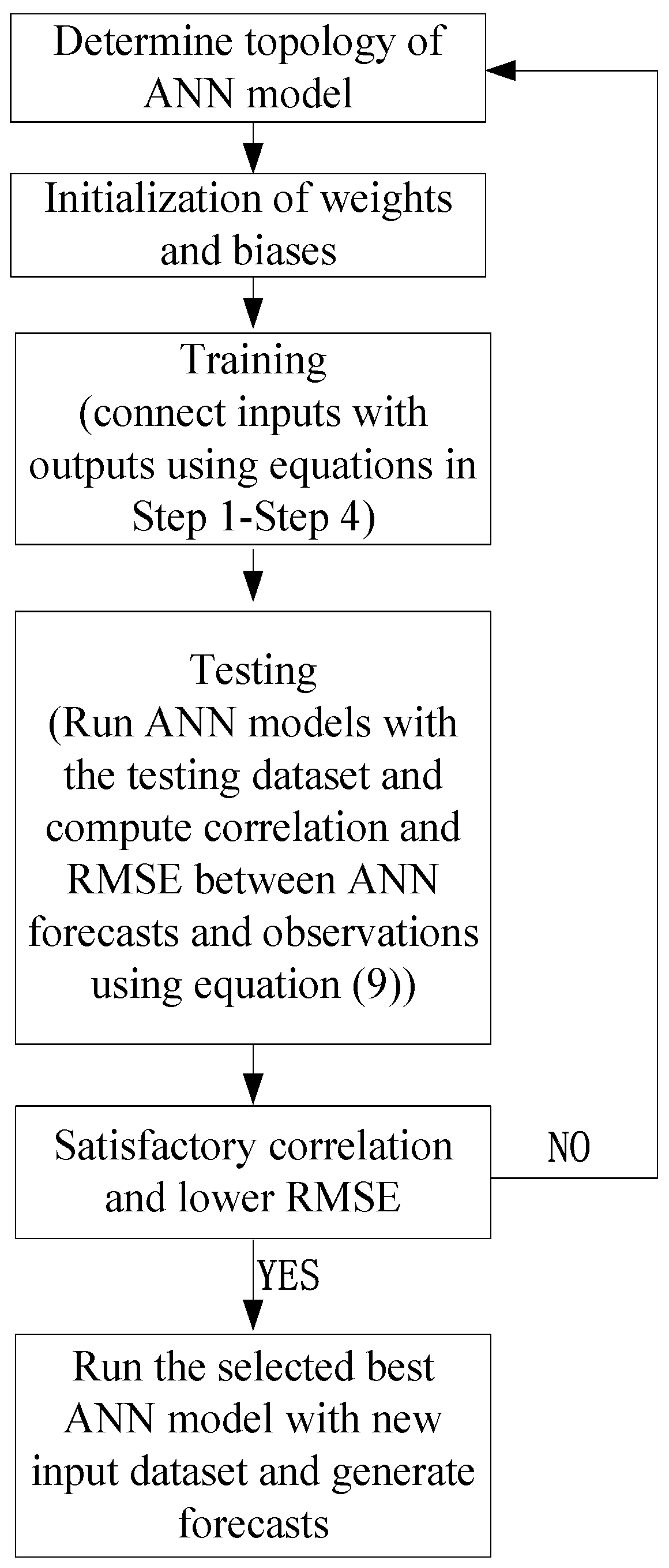
3.2. Training and Testing
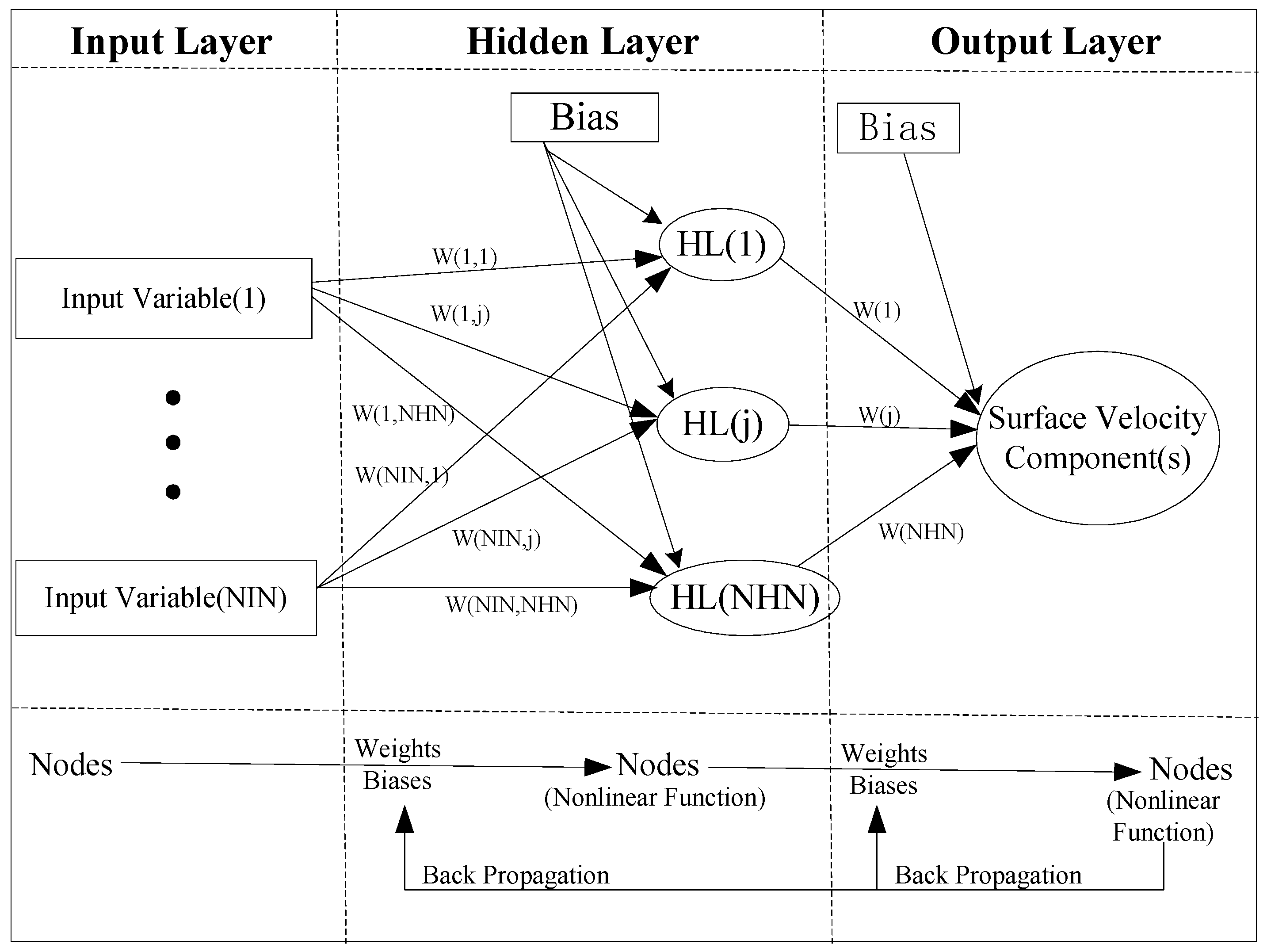
To avoid the “over-fitting problem” while training ANN models, the number of nodes in the hidden layer was determined using the formula proposed by Huang and Foo [
62]:
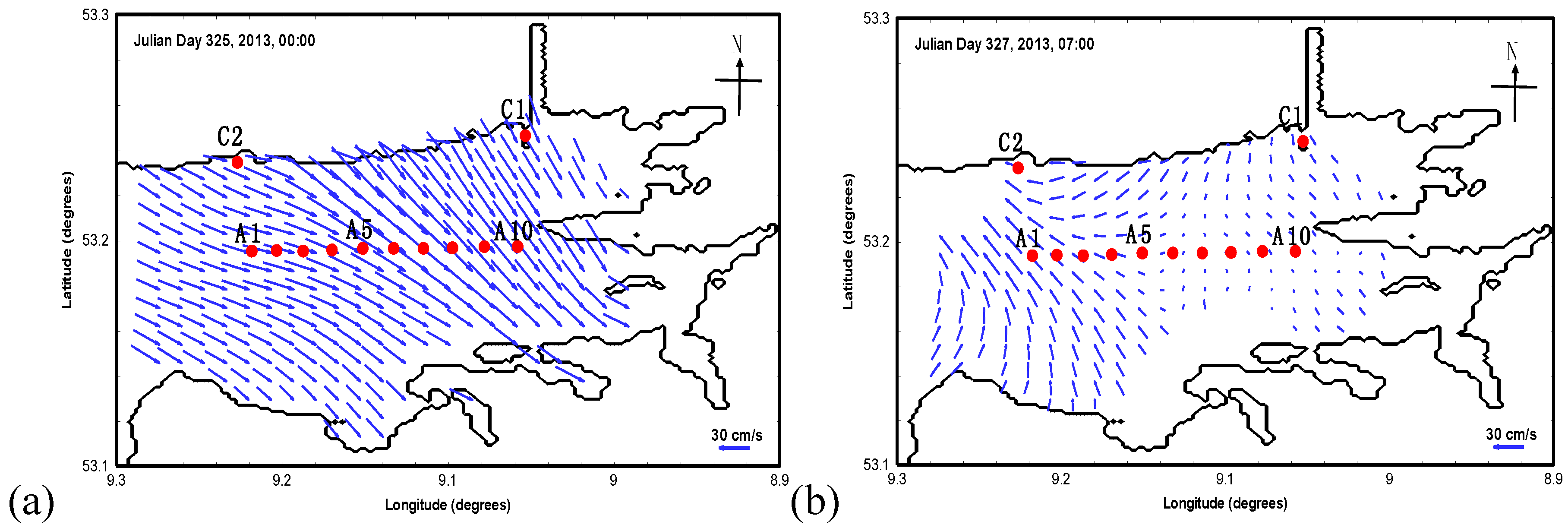
Surface current components at ten points (see
Figure 1) covered by the radar system with high coverage density were separately used to develop the ANN models. The choice of appropriate input variables is most important. Tests of input variable topology were undertaken for
u and
v components of surface velocity, respectively. Different input structures were assessed using the testing dataset as presented in
Table 4 and
Table 5, the number of input variables were increased by adding longer historical observation of corresponding radar velocity component. To compare and determine appropriate input variable structures when developing ANN models, magnitudes of correlation (R), bias, RMSE and RSE were averaged at points A1–A10 for
u and
v velocity components, respectively, as presented in
Table 4 and
Table 5. Model U1 only considers tidal elevation, wind speeds and directions as input variables to establish an ANN forecast model. Models U2–U12 in addition to the above three input variables also consider historical radar observations over different periods as input variables. The length of historical radar data varied from one hour
to six hours
, corresponding to Models U2 to U12.
Table 4 shows that the ANN models for the
u velocity component using historical velocity components as input variables can increase forecasting accuracy compared with Model U1, except for Model U5 had comparable statistics with Model U1. In general, for cases when only one historical velocity component was included (i.e., Models U2–U7), model performance deteriorated as historical data at more distant time steps were used. The averaged RMSE of the
u velocity component at the ten locations between model results and radar measurements is relatively large in Models U1 and U5 at around 15.90 cm/s, while the averaged RMSE values are less than 10 cm/s in Models U2–U3 and U8–U12. Moreover, for these models including historical data at (
t − 1) or (
t − 2) were involved as input variables, high correlation (greater than 0.68) exists. Improvement of averaged RMSE at the ten analysis locations is greater than 38% (Model U3 vs. U1) for
u velocity component in comparison with Model U1. The maximum improvement of averaged RMSE is 71% (Model U8 vs. U1) among these models. Values of RSE were less than or equal to 40% except for Model U1. The minimum value of RSE existed in Models U8, U9 and U11 (9%). This indicates that consideration of historical
u velocity components at (
t − 1) or (
t − 2) in ANN models significantly improved model performance and accuracy. However, results of Models U1 and U4–U7 deviated greatly from radar observations. This illustrated that consideration of historical radar data at (
t − 3) or more previous time steps did not have positive effects on ANN model performance.
Models U8–U12, as presented in
Table 4, were developed to examine whether combination of historical data over longer period can enhance model performance. Models U8, U9 and U11 outperformed Model U2 based on RMSE values and correlation. These results are encouraging and suggest that use of historical data over a longer period can improve model accuracy. Although performance of Models U10 and U12 was not as good as Model U2, correlations between radar data and results of these models were the same and high (0.94). In short, involving of historical data over longer period was a potential way to increase ANN model accuracy for
u velocity component.
The same study on topology of input variables was employed for
v velocity component as presented in
Table 5. Model V1 considers only tidal elevation, wind speeds and directions as input variables to establish ANN forecast model. Models V2–V12 in addition to the three input variables also consider historical radar observations as input variables. The length of historical radar data varied for corresponding Models V2–V12.
Averaged statistics in
Table 5 show that ANN models for the
v velocity component considering historical velocity components as input variables can increase forecasting performance. When radar data at one historical time step were involved as input variables (Models V2–V7), model accuracy deteriorated as data at more distant time steps were used. Averaged RMSE values between model results and radar measurements at the ten locations is very large in Model V1 at 12.74 cm/s, while it is less in models (Models V2–V7) with data from one historical time step. Correlation between radar data and ANN model results was high (greater than 0.68) in Model V2 and V3. However, performance of Models V4–V7 was not considered good and with results approaching values achieved by Model V1. Results indicate that using historical data at (
t − 1) or (
t − 2) can increase model accuracy.
To further explore sensitivity of input variable structure on model performance, sensitivity models involving historical data over longer periods were examined (see Models V8–V12). Performance of Models V8–V12 was better than or comparable with the Model V2 based on RMSE values. The maximum improvement in RMSE was 61% (V9 vs. V1). Additionally, values of correlation between radar data and results in Models V8–V12 were greater than or equal to that of Model V2 (0.89). Values of RSE were less than or equal to 22% in these models. The minimum value of RSE existed in Models V9 and V11 (18%). The above analysis illustrates that consideration of historical radar data over longer periods with time steps less than (t − 5) positively contributed to improve model performance and accuracy. It was a potential and meaningful way to use more historical data as input variables.
The above tests for both u and v velocity components at ten locations with different structures of input variables show that the best ANN model for u and v velocity component forecasts are Models U8 and V9, respectively. Both can generate acceptably good results compared with radar data. The difference between the input variable structures of Model U8 and V9 is due to the fact that wind stresses have more influence on the v component of surface velocity than on the u component. It is seen that the addition of one extra historical data (v(t − 3)) helped Model V9 generate better results; Model U8, forecasting the more tidally dominated u component, was able to generate satisfactory results using less historical data. It is significant to observe that the ANN approach is sensitive to dominant physical processed in such an environment.
3.3. Forecasts of Surface Velocities
To examine the performance of the best-developed ANN Models U8 and V9 with one-hour forecasting lead-time, the predicted surface current components at location A3 and A8 (see
Figure 1) are shown in
Figure 6,
Figure 7,
Figure 8 and
Figure 9.
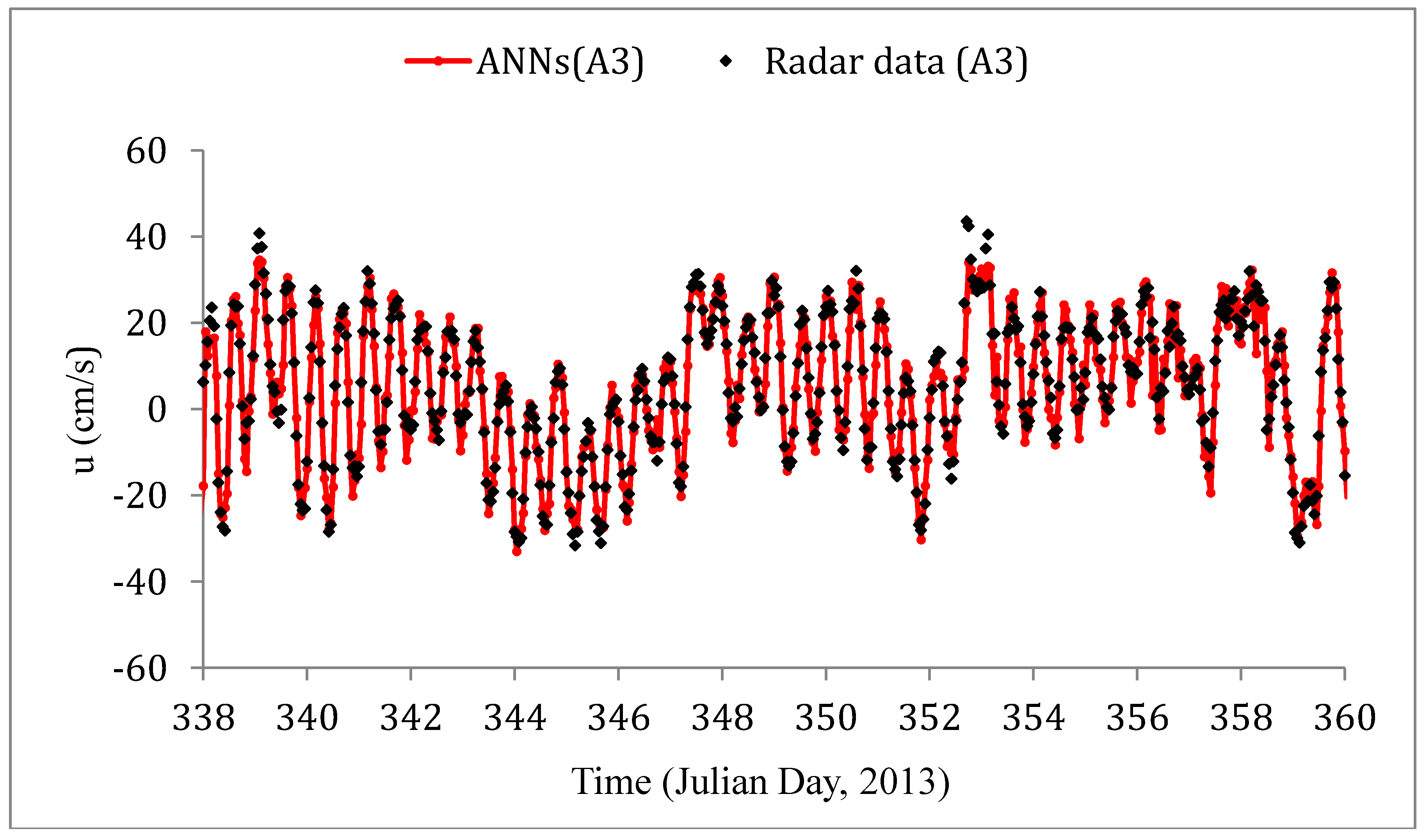
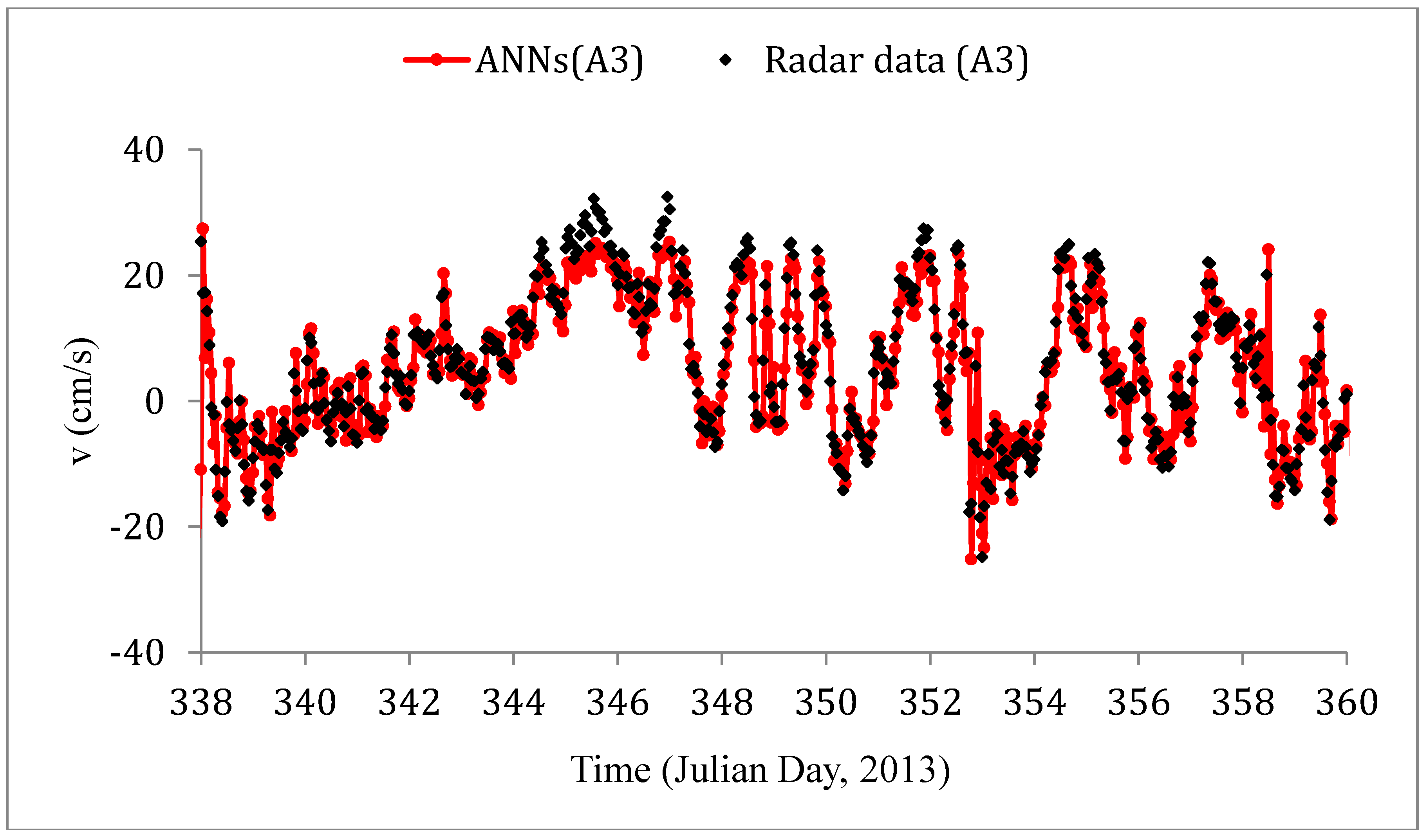
Figure 6 and
Figure 7 show that Models U8 and V9 can produce good agreement for corresponding east–west and north–south velocity components in comparison with radar data over a long forecast period (approximately 28 days) at location A3 with a one-hour forecasting lead time. Significant deviation exists only at a few time steps, such as Julian Days 352–354 for
u velocity component (see
Figure 6) and Julian Days 345–347 for
v velocity component (see
Figure 7). Correlation coefficients for both surface velocity components between predicted results and radar data at location A3 are greater than 0.92.
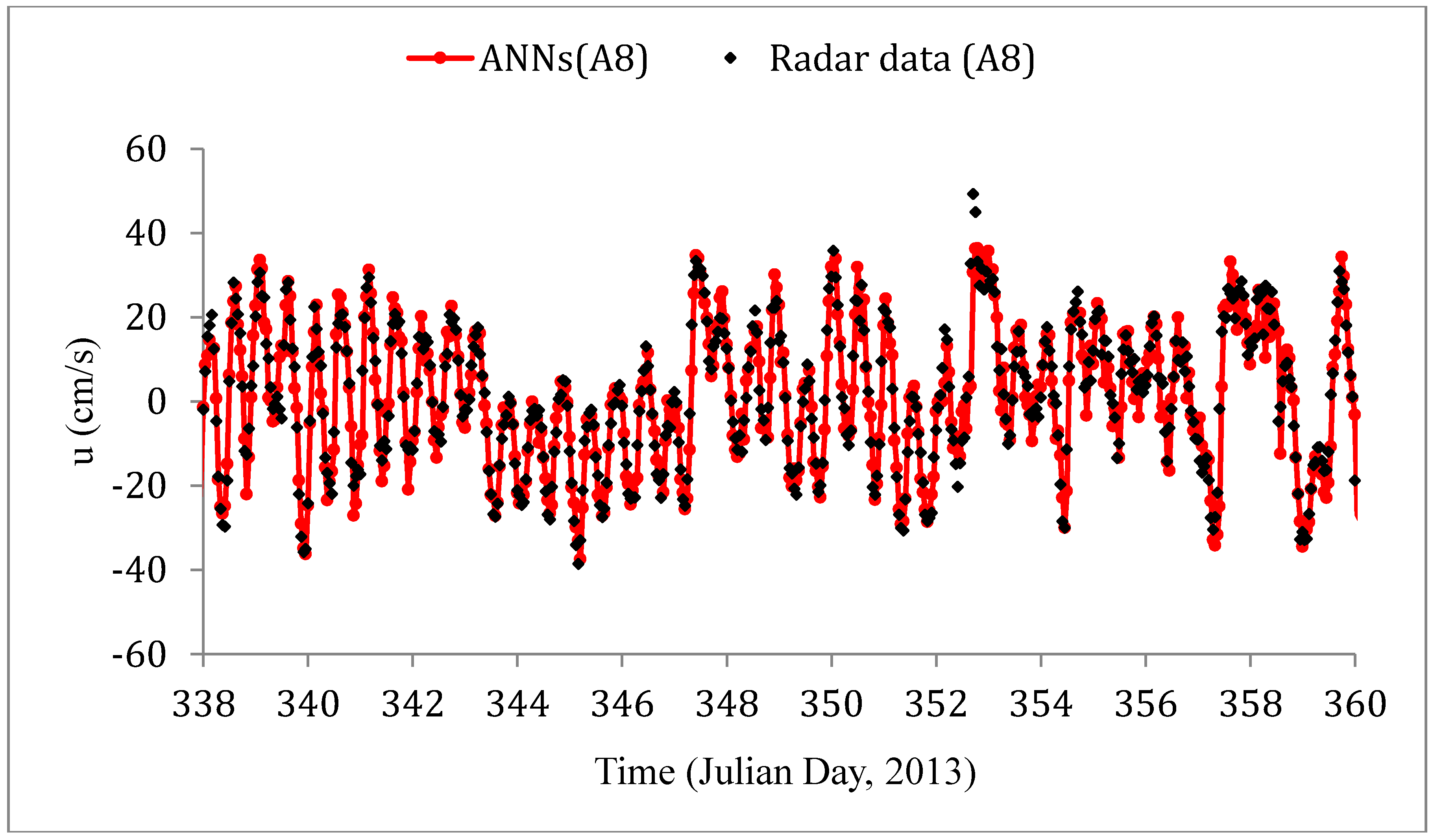
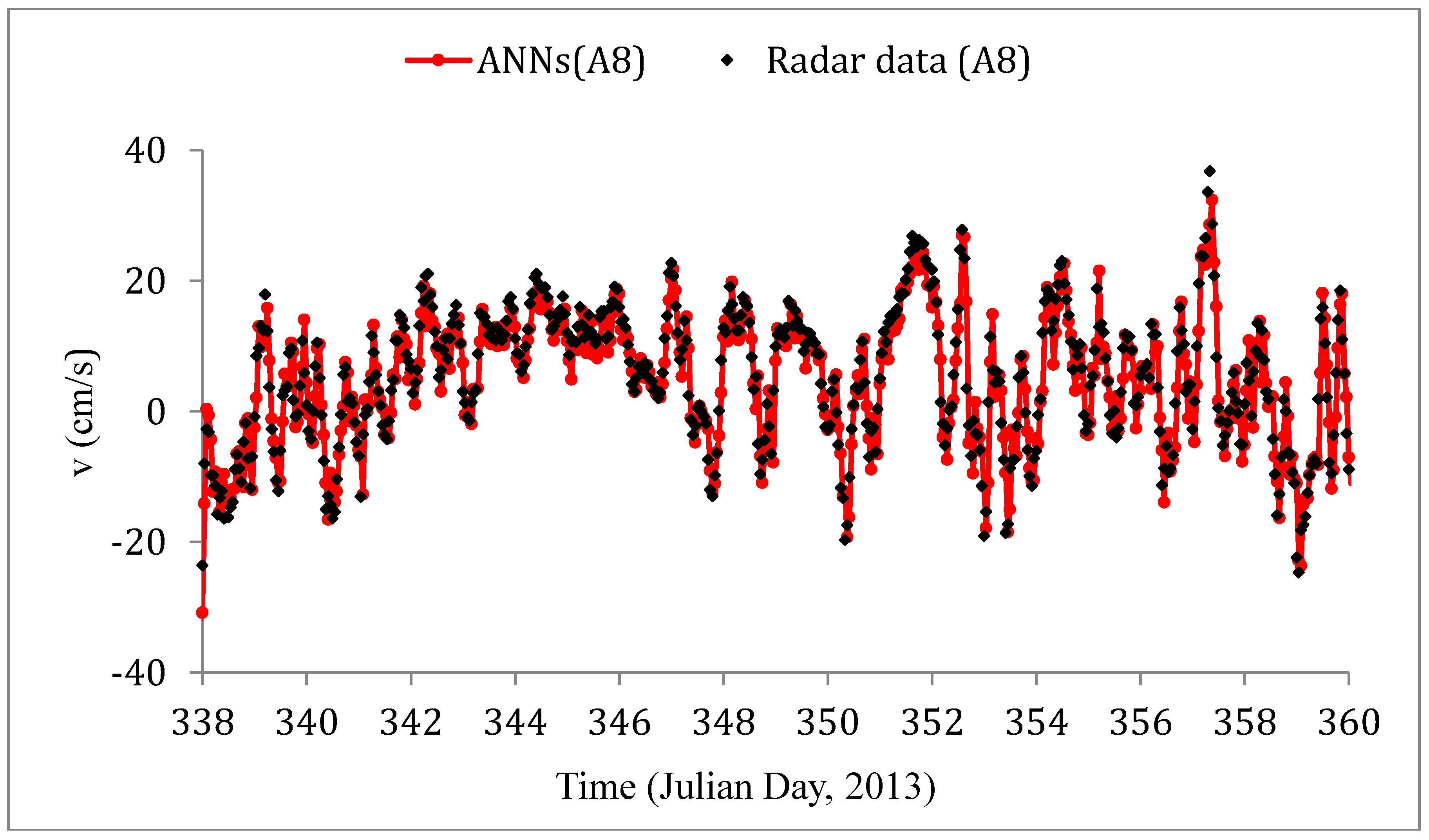
Figure 8 and
Figure 9 show that Models U8 and V9 can produce forecast of both surface velocity components having high correlation with radar data over a long forecast period at location A8 with one-hour forecasting lead-time as well. Again, significant deviation exists at only a few time steps, such as Julian Days 352–354 for
u velocity component and Julian Days 352–353 for
v velocity component. Correlation coefficients for both surface velocity components between predicted results and radar data at location A8 are greater than 0.93.
To quantitatively assess model forecasts at each of the output locations within Galway Bay, values of RMSE, bias, correlation coefficient (R) and RSE of forecasts from ANN models using the forecast dataset for 670 h at each location are computed using Equations (1)–(4) and presented in
Table 6 and
Table 7.
Table 6 shows that the range of RMSE between forecasts of
u velocity component from Model U8 and radar data at ten locations is 4.29–5.15 cm/s. Additionally, the range of
u velocity components at ten points is −41.9–49.9 cm/s, as presented in
Table 3. RMSE between ANN forecasts and radar data was less than 5% of the
u velocity component range on average. Correlation coefficient is equal to or greater than 0.95 at all locations. This indicates that Model U8 using tidal elevation forecast, wind speeds and directions, and historical
u velocity components at previous two hours as input variables is capable of yielding satisfactory forecasts in domain.
Table 7 shows that the range of RMSE values of
v velocity component between results from Model V9 and radar data at ten locations is 3.69–5.66 cm/s. Moreover, the range of
v velocity components at the points is −40.4 to 57.8 cm/s, as presented in
Table 3. RMSE between ANN forecasts and radar data was less than 5% of the
v velocity component range on average. Correlation coefficients are equal to or greater than 0.90 at all locations. This indicates that Model V9 with input variables including tidal elevation forecast, wind speeds and directions, and historical
v velocity components at previous three hours has an ability to generate good forecasts in the domain.
Forecasts of
u velocity components from Model U8 have higher correlations with radar data (
Table 6) than for
v velocity component from Model V9 (
Table 7) at all analysis locations. The range of the RMSE values of
v velocity components is greater than for the
u velocity components. Absolute values of bias in
v velocity components are greater than
u velocity components. This suggests that more significant satisfactory forecasts of east–west flows can be produced by Model U8 than north–south flows by Model V9. This may be because tide-induced flows in the east–west in direction are more deterministic than the strongly wind dominated north–south flows which are more random in nature. Generally, values of RSE for
u velocity components at the ten analysis points were smaller than those of the
v velocity component. Again, this indicates that Model U8 produced more accurate predictions than Model V9.
The forecasting window of the ANN Models U8 and V9 is one hour. However, a longer forecasting window is desirable for various practical applications such as search and rescue and oil spill response. To examine the influence of adopting historical data as input variables on ANN model performance and to extend forecast window, experiments on forecasting windows for both surface velocity components at the ten analysis locations were performed in the following section.
3.4. Forecasting Window Tests
To generate satisfactory forecasts over a longer forecasting window, tidal elevation, wind speeds and directions at different historical time steps were used as input variables in additional test Models U13–U19 and V13–V19, as presented in
Table 8 and
Table 9. Since Galway Bay hydrodynamics are affected by semi-diurnal periodic tides [
37], radar data of velocity components, wind speed and direction 12 h before the prediction time t were also examined as input variables to assess sensitivity of results in Models U17–U19 and V17–V19. Input variable structures and averaged values of RMSE, bias, R and RSE using the testing dataset are computed using Equations (1)–(4) and are presented in
Table 8 and
Table 9 corresponding to the
u and
v velocity, respectively.
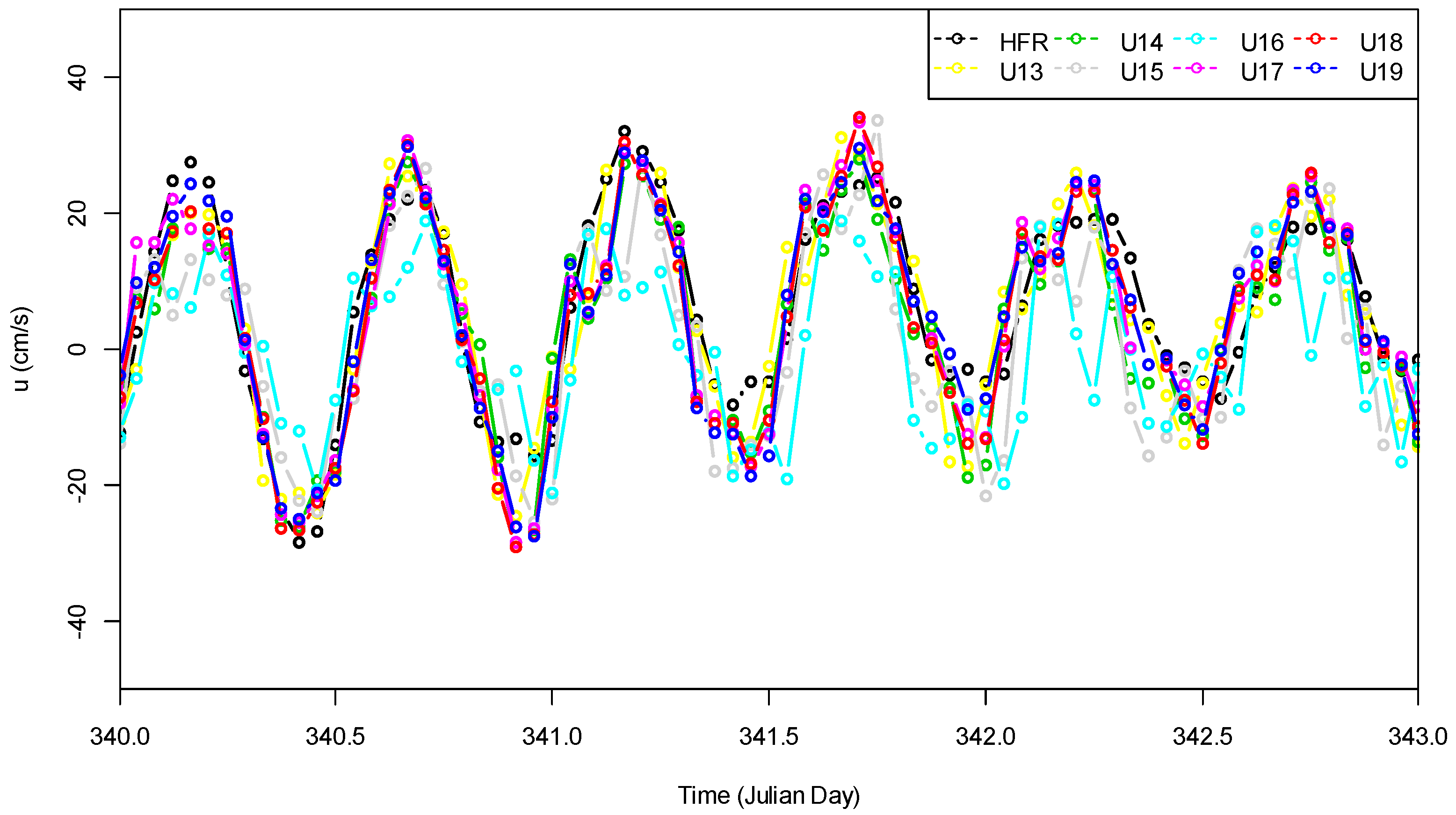
Table 8 and
Table 9 show averaged values of RMSE between radar data and ANN model forecasts at the ten analysis locations. In general, values of RMSE increase as the forecasting window becomes longer; and correlation between radar data and predicted results deteriorate significantly as the forecasting window becomes longer (U13–U16 and V13–V16). This is because auto-correlations among
u components of surface currents are stronger when the lag is smaller. Based on a correlation assessment system, as proposed by Taylor [
63], high correlation (greater than 0.68) exists in Models U13, U14 and V13. This indicates that Model U14 using historical data (
) is capable of producing satisfactory forecasts for the
u velocity component. Values of RMSE between testing dataset (20% of the full dataset) and radar data as presented in
Table 8 increase significantly from Model U13 to Model U16. Model V13 using historical data (
) can yield satisfactory forecasts for
v component of surface velocity. Model U14 with a three-hour forecasting window and Model V13 with a two-hour forecasting window can generate closer results to HFR data with high correlation (≥0.75). RMSE values in Models U13, U14 and V13 were better or comparable with Eulerian RMSE value (9 cm/s) in the first 6 h forecasts obtained by Frolov et al. [
36]. To compare and evaluate forecasts, forecasts of surface velocity components are compared with radar data at the location A3. as shown in
Figure 10 and
Figure 11 respectively.
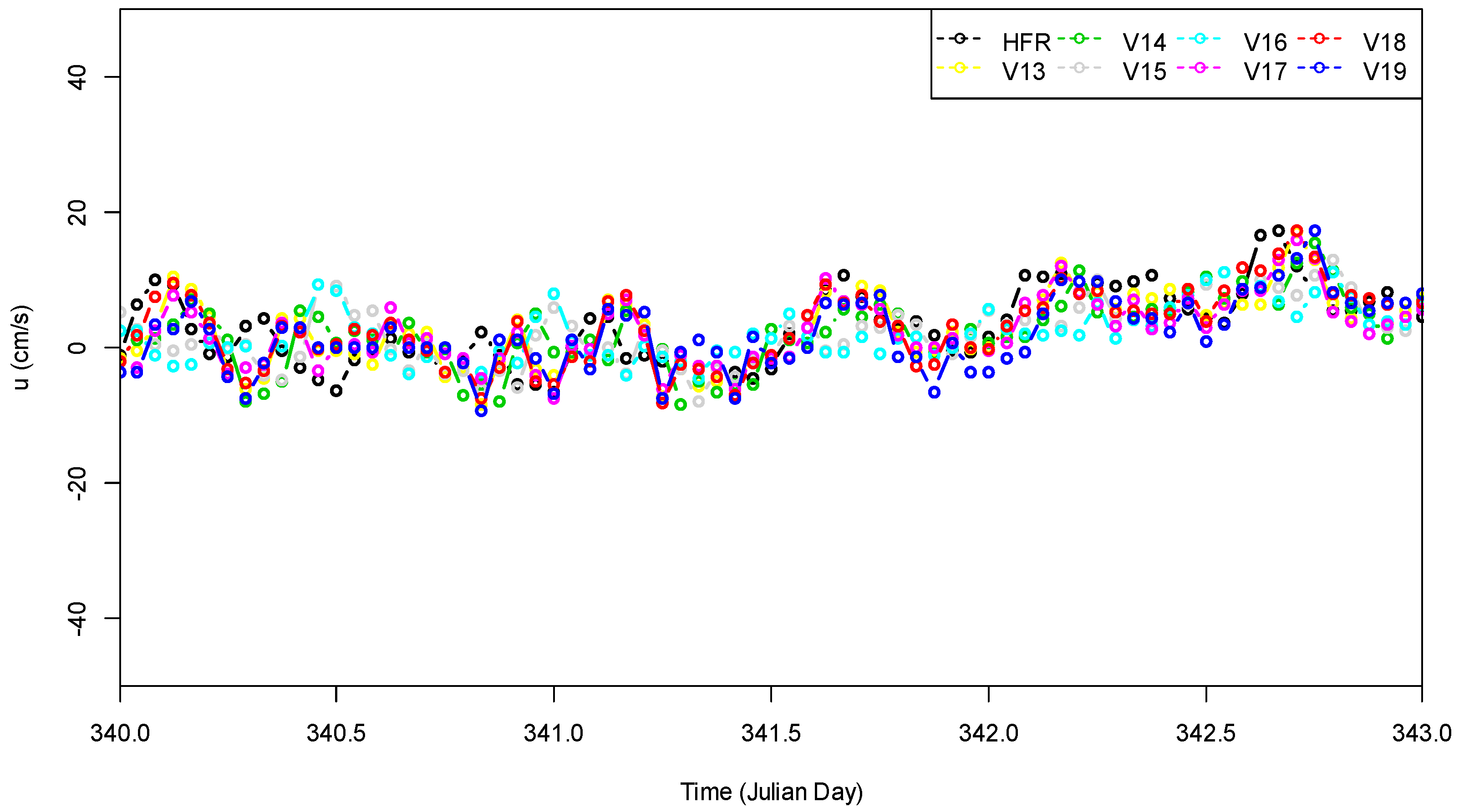
Based on the good performance of Models U14 and V13, Models U17–U19 and V17–V19 as presented in
Table 8 and
Table 9 were used to assess model accuracy through considering tidal elevation, historical HFR data, wind speed and wind direction 12 h before forecasting time t as input variables. Statistics in
Table 8 illustrate that Models U17 and U18, using tidal elevation or wind speed 12 h prior, slightly enhance model performance for
u velocity components in comparison with U9. Improvement of RMSE for
u velocity component in Model U17 is 5% relative to Model U14.
Table 9 shows that the addition of velocity component and wind speed 12 h before time t slightly affects model performance (see Model V13 vs. Model V18); however, when wind direction at the previous 12 h is included, model performance deteriorates (see Model V18 vs. Model V19). This may be because variations in wind direction occur quickly. It is observed that by including wind direction 12 h before forecast time does not have a strong positive influence on surface current forecasts. The best forecasting ANN models having a relatively long forecasting window are Models U17 and V18, as shown in
Figure 10 and
Figure 11. Additionally, the value of RSE in Model V19 was significantly increased when including wind direction 12 h before the forecasting time.
In general, good agreement exists between the radar data and forecasts from Model V18. Averaged correlation coefficient of u velocity component between radar data and ANN predictions at the ten analysis points using the same input structure as Model U17 is greater than 0.8, the value of averaged correlation coefficient at the ten analysis points is greater than 0.77 for v velocity component using the same input structure as Model V18.
The authors previously developed hydrodynamic models of Galway Bay and used data assimilation (DA) to assimilate radar data into the model to improve model results; these models were then used to generate forecasts of surface currents. Ren and Hartnett [
5] and Ren et al. [
3] used Optimal Interpolation data assimilation algorithm and assimilation of indirect correction of wind stress. Here, we compare the forecasts obtained using the simpler ANN models to forecasts using DA models. Models U17 and V18 were used to produce prediction of surface velocity components at A3 during the same forecasting period as the best data assimilation models from Ren and Hartnett [
5] and Ren et al. [
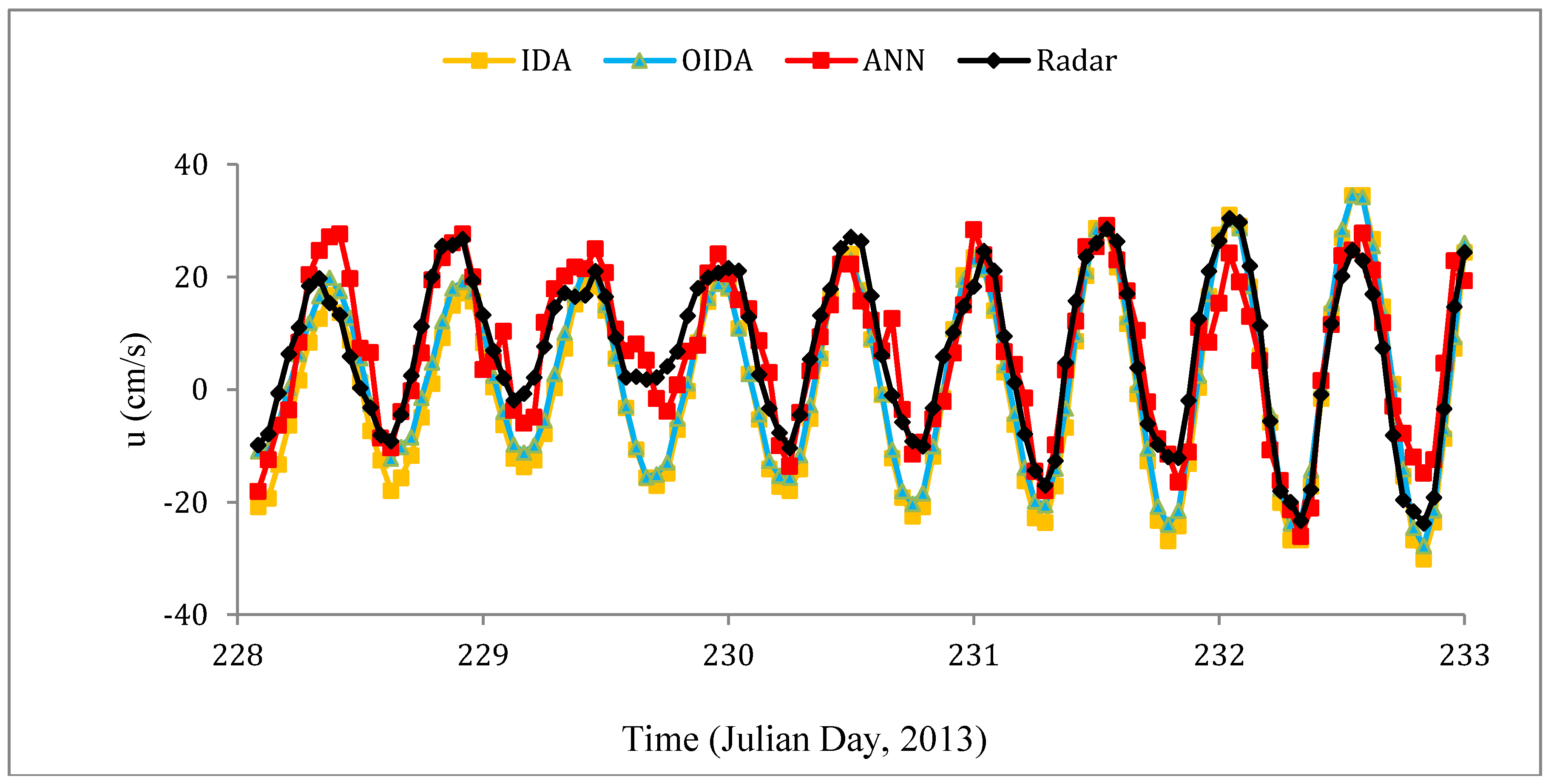
3]. Time series of prediction for both surface velocity components are shown in
Figure 12 and
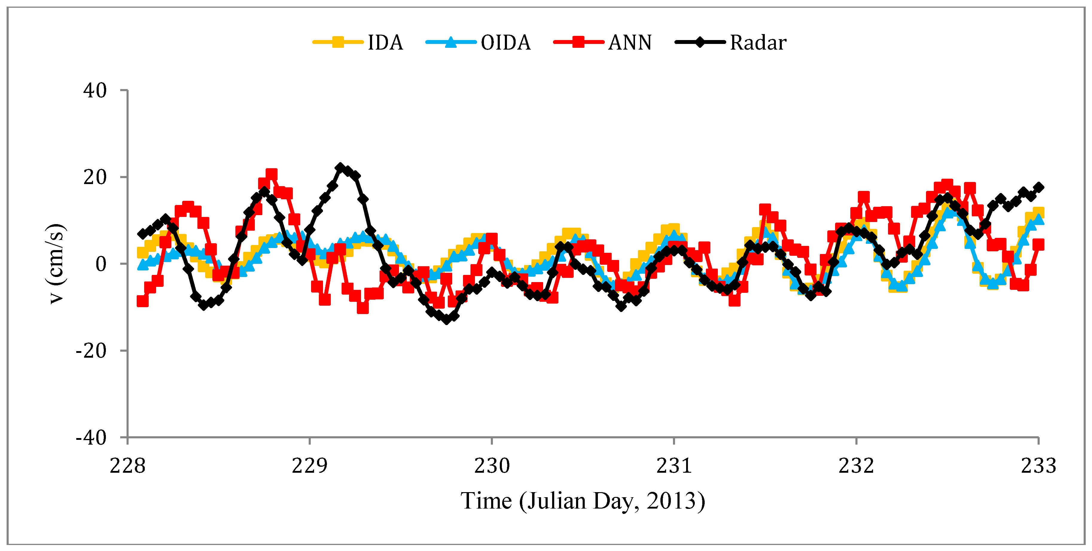
Figure 13.
Figure 12 illustrates that ANN Model U17 generally outperformed data assimilation models using Optimal Interpolation and indirectly correction of wind stress. Better performance from ANN models is significant at peak times of surface east–west velocity component. RMSE values between model results and radar data during the five-day period are presented in
Table 10.
Table 10 shows that ANN Model V18 produces consistently better predictions than the data assimilation models. Improvement in RMSE for
u and
v velocity component is 36% and 11%, respectively, relative to the IDA model results, and 22% and 12%, respectively, relative to the OIDA model results. Moreover, the computational costs of the ANN model were significantly lower than data assimilation models; this is very attractive for forecasting systems.
4. Discussion
The ANN models developed for both surface velocity components using tidal water elevation, wind speeds and direction, and historical radar surface currents are capable of generating short-term forecasts of surface currents with high accuracy during a 3-h forecasting window. Significant aspects of this research are: historical radar data were applied to produce forecasts of surface currents using ANN algorithm at a range of locations over a large domain; the input variable structure was assessed by analyzing the results of a range of input variables; the practical forecasting window of surface velocity components was extended by choosing “older” historical radar data; and performance of predictions was evaluated in comparison with radar data over a relatively long period. The ANN forecast models could be used for activities such as gap filling of radar data, oil spill response and search and rescue. The short-term forecasts developed herein are more accurate than attempts made by previous research efforts. Correlation coefficients of
u velocity component between ANN forecasts and radar data over 670 h were greater than 0.95 at all analysis points, as presented in
Table 6. Correlation coefficients of
v velocity component were greater than 0.90 as presented in
Table 7. These correlation values were greater than those (0.76–0.79) produced by Mathew and Deo [
64] using ANN, Decision Tree and nonlinear regression to predict wind speeds.
Saha et al. [
61] also used ANN to generate forecasts of surface currents using results from a hybrid coordinate ocean model (HYCOM) and oceanographic buoy observations. The use of a model as input to the ANN forecasts is a significant difference from the approach adopted by the authors; the authors’ approach is an attractive alternative since it does not rely on computational requirements and hence is more efficient.
RMSE values of surface
u and
v velocity components between the model forecasts and observations over different lead time obtained by Saha et al. [
61] were in the order of 15.89 cm/s and 15.21 cm/s, respectively, which are generally larger than the averaged RMSE values obtained in this research at ten location over a wide range using Models U17 and V18 for surface
u and
v components separately by 10.05 cm/s and 7.91 cm/s. As lead-time became longer, RMSE values in their study increased. Correlation coefficients of
u velocity component between model predictions and observations obtained by Saha et al. [
61] ranging from 0.82 to 0.93 are stronger than the value in this research from Model U17 (0.77); however, Model V18 in this research had a stronger correlation coefficient (0.75) for velocity
v component than those correlation coefficients when the lead time was greater than three days in the study by Saha et al. [
61]. This is particularly encouraging since the authors’ forecast did not use a detailed numerical model as input.
Furthermore, according to the RMSE between ANN model results and observations, forecasts of surface currents produced in this research were significantly better than vertical currents at depths generated by Aydogan et al. [
14], in which RMSE was greater than 10 cm/s and 16 cm/s on average for
u and
v velocity components, respectively. In addition, the correlation coefficient of velocity
u component (0.95) between results from Model U8 and HFR data was better than that value (0.93) obtained by Gauci et al. [
34] for radar data gap filling; however, their correlation coefficient (0.93) was slightly better than that value (0.91) for velocity
v component between results from Model V9 and HFR data. Thus, the accuracy achieved by the authors when forecasting is of the same order obtained by others in gap filling (in effect hindcasting), which is an easier process using data available at the time of interest rather than forecasting.
This is the first time that research has been developed using ANN to extend forecasting windows using historical HFR data. Comparative studies presented in
Table 8 and
Table 9 show that using HFR data
and
,
as input variables within ANN models produce satisfactory forecasts for
u and
v velocity components, respectively.
5. Conclusions
In this research, an ANN technique was employed to establish predictive models for surface currents in Galway Bay. Tidal elevations, radar data wind speeds and directions were chosen as input variables for an ANN predictive model. Based on previous studies, and to further extend model forecast ability, surface velocity components from radars at previous observation time steps were used as input variables and tested. u and v components of surface velocities were the output variables of the ANN models. The results indicate that an ANN approach can produce satisfactory correlations for both surface velocity components. ANN models can generate high-accuracy forecasts of both surface velocity components over short term durations. The main conclusions from this research are:
- (a)
Incorporating historical radar measurements as input variables can produce high accuracy forecasts with a one-hour forecasting window. Correlation coefficients between predicted results and HFR data are greater than or equal to 0.95 for
u velocity components. Correlation coefficients are greater than or equal to 0.90 for
v velocity components. Using the above objective measures, these forecasts represent very high degrees of accuracy [
63].
- (b)
Very strong correlations (equal to or greater than 0.90) and small RMSE values at ten locations for both u and v components of surface currents show that ANN algorithms can be used as a powerful tool to predict surface currents with one-hour forecasting window at single/multiple points or over a domain. Thus, forecasts of surface flow fields throughout a domain can be obtained when historical radar observations are available. This can also be used for filling radar observation gaps due to variation in environmental conditions, which has significant implications for analysis and presentation of coastal radar data.
- (c)
A models are capable of producing satisfactory forecasts over a three-hour forecasting window for
u component of surface velocity. As expected, correlation coefficients decrease with increasing forecasting window. Strong correlations (i.e., 0.75 greater than 0.68 for significance proposed by Taylor [
63]) are achieved when the forecasting window is equal to or less than three hours. Satisfactory forecasts of
v component of surface velocity can be obtained from ANN models when a forecasting window is equal to or less than two hours. Correlation of
v velocity component between observations and model results has a negative trend as the forecasting window increases.
- (d)
RMSE values and a skill score assessment show that ANN models outperformed complex, computationally expensive data assimilation models using: (i) optimal interpolation; and (ii) indirect correction of wind stress.
- (e)
Once an ANN model has been established and verified, forecasts can be efficiently generated for a wide range of environmental forcing conditions. ANN algorithms provide a promising approach for the development of forecasting models due to computational efficiency, ease of implementation and accuracy.
Results indicate that ANN models can generate short-term accurate forecasts for surface velocity components. Such forecasting has many real world applications such as hindcasting/reanalysis; providing accurate and real-time information for search and rescue and oil spill response; generating forecasts of currents at marine renewable turbine test site; and hydro-environmental monitoring. Since spatial coverage of the radar surface vector fields varies over time, ANN models can be adopted to accurately fill measurement gaps in time and space. In summary, the application of HFR data within ANN algorithms under appropriate considerations provides a very useful approach to generate forecasts of surface velocity components. It is important that the structure of input variables is carefully examined when ANN model is used to forecast surface currents in other domains.
In future research, the authors are interested in using numerical model results as ANN inputs when HFR data are not available to develop hybrid ANN models.


