Article

Radar Path Delay Effects in Volcanic Gas Plumes: The Case of Láscar Volcano, Northern Chile

by
Stefan Bredemeyer
1,*,
Franz-Georg Ulmer
2,
Thor H. Hansteen
1 and
Thomas R. Walter
3
1
GEOMAR Helmholtz Centre for Ocean Research Kiel, Research Division 4: Dynamics of the Ocean Floor, Wischhofstr. 1–3, 24148 Kiel, Germany
2
German Aerospace Center (DLR), Remote Sensing Technology Institute, Oberpaffenhofen, 82234 Weßling, Germany
3
GFZ German Research Centre for Geosciences, Section 2.1: Physics of Volcanoes and Earthquakes, Telegrafenberg, 14473 Potsdam, Germany
*
Author to whom correspondence should be addressed.
Remote Sens. 2018, 10(10), 1514; https://doi.org/10.3390/rs10101514
Submission received: 28 August 2018 / Accepted: 18 September 2018 / Published: 21 September 2018
(This article belongs to the Special Issue Remote Sensing of Volcanic Processes and Risk)

Abstract

:
Modern volcano monitoring commonly involves Interferometric Synthetic Aperture Radar (InSAR) measurements to identify ground motions caused by volcanic activity. However, InSAR is largely affected by changes in atmospheric refractivity, in particular by changes which can be attributed to the distribution of water (H2O) vapor in the atmospheric column. Gas emissions from continuously degassing volcanoes contain abundant water vapor and thus produce variations in the atmospheric water vapor content above and downwind of the volcano, which are notably well captured by short-wavelength X-band SAR systems. These variations may in turn cause differential phase errors in volcano deformation estimates due to excess radar path delay effects within the volcanic gas plume. Inversely, if these radar path delay effects are better understood, they may be even used for monitoring degassing activity, by means of the precipitable water vapor (PWV) content in the plume at the time of SAR acquisitions, which may provide essential information on gas plume dispersion and the state of volcanic and hydrothermal activity. In this work we investigate the radar path delays that were generated by water vapor contained in the volcanic gas plume of the persistently degassing Láscar volcano, which is located in the dry Atacama Desert of Northern Chile. We estimate water vapor contents based on sulfur dioxide (SO2) emission measurements from a scanning UV spectrometer (Mini-DOAS) station installed at Láscar volcano, which were scaled by H2O/SO2 molar mixing ratios obtained during a multi-component Gas Analyzer System (Multi-GAS) survey on the crater rim of the volcano. To calculate the water vapor content in the downwind portion of the plume, where an increase of water vapor is expected, we further applied a correction involving estimation of potential evaporation rates of water droplets governed by turbulent mixing of the condensed volcanic plume with the dry atmosphere. Based on these estimates we obtain daily average PWV contents inside the volcanic gas plume of 0.2–2.5 mm equivalent water column, which translates to a slant wet delay (SWD) in DInSAR data of 1.6–20 mm. We used these estimates in combination with our high resolution TerraSAR-X DInSAR observations at Láscar volcano, in order to demonstrate the occurrence of repeated atmospheric delay patterns that were generated by volcanic gas emissions. We show that gas plume related refractivity changes are significant and detectable in DInSAR measurements. Implications are two-fold: X-band satellite radar observations also contain information on the degassing state of a volcano, while deformation signals need to be interpreted with care, which has relevance for volcano observations at Láscar and for other sites worldwide.

Graphical Abstract

1. Introduction

Volcano monitoring is effectively based on multi-parametric datasets, often characterizing surface deformation, degassing, seismicity and temperature changes in time and space. However, even though comparison of independent datasets is common, they are only rarely integrated into a common evaluation scheme to enhance the relative strengths of the individual applied methods. Seismic and deformation data for instance are increasingly being integrated to improve spatio-temporal localization of magma movement beneath a volcano, which enables to better constrain the geometries of magma pathways and reservoirs, and to derive more precise physical models of the associated processes [1,2]. Gas emission and deformation data, however, have not yet been deeply considered as integrated information, though it has been shown that variations in degassing and deformation are often intimately coupled [3]. A combined analysis of time series measurements of volcanic degassing and deformation rates proved to be a powerful tool for the evaluation of volumetric changes in magma reservoirs due to the accumulation or discharge of volcanic gases (e.g., [4,5]). Dynamics of degassing are furthermore critical for understanding pressure fluctuations in a magmatic and hydrothermal system, which additionally may manifest as temporary deformation of the volcanic edifice [6,7,8]. However, these datasets are commonly considered separately, and the fate of gas emissions downwind of the emission source is typically not taken into account, which is why the contribution of gas emissions on the radar signal used for deformation measurements has not been comprehensively demonstrated. Differential interferometric synthetic aperture radar (DInSAR) measurements allow for the detection of mm-scale line of sight (LOS) displacements of the observed surface [9]. It has been well demonstrated that the accuracy of satellite radar ground deformation measurements is affected by changes in atmospheric refractivity, in particular by changes which can be attributed to the highly variable distribution of water vapor in the observed atmospheric column [10,11].
Atmospheric contributions to DInSAR data often have similar magnitudes and wavelengths as the actual ground deformation signal, and thus they need to be removed from interferograms, when deformation measurements are the purpose of monitoring. There have been two main strategies for this, (i) time-space-based filtering, and (ii) modeling of atmospheric contribution [12]. In particular, the latter is highly successful, as interfering contributions from a moist atmosphere can coarsely be predicted and compensated by means of high-resolution numerical weather models (e.g., MM5, and WRF), which provide the information required to predict the atmospheric phase delay in the LOS of an interferometric measurement [13,14,15,16].
Degassing volcanoes; however, produce their own atmospheric disturbances, which are typically not well captured by weather models [17,18]. The large and variable amounts of water vapor in volcanic plumes may cause differential phase errors in interferometric measurements due to reduction of radar propagation velocity within the plume above and downwind of the volcano [19,20,21,22].
The leeward sector of a degassing volcano is hence prone to be affected by pronounced differential phase signatures, which can be misinterpreted as a deforming ground surface, and may thus obscure the real ground deformation information of an interferogram. Rosen et al. [19] described the possible consequences that such propagation delays would have on DInSAR measurements using the examples of phase signatures that occurred on Kilauea volcano, Hawaii. Similarly, Wadge et al. [20] observed enhanced tropospheric delays in radar data of Soufrière Hills. Instead of using weather models for the correction of their DInSAR data, these authors exploited data from Global Positioning System (GPS) measurements on the leeward side of the volcano. Based on local SO2 flux and gas compositional measurements, and assuming a homogeneous distribution of water vapor inside the volcanic gas plume, they however obtained an estimate of the gas plume related radar delay of only about 0.05 mm, which is far below, and thus negligible with respect to InSAR resolution. Gas plume related disturbances are nevertheless also identified elsewhere in interferograms of degassing volcanoes (e.g., at Pico do Fogo as described in González et al. [21]), but remained to be quantitatively demonstrated and validated for a selected showcase.
To reach this aim, the precipitable water vapor (PWV) content in the plume at the time of SAR acquisitions has to be determined. PWV is the amount of water vapor (in kg·m−2 or mm) vertically integrated in an atmospheric column. Space borne radar interferometric delay measurements in principle can be used to map the spatial distribution of water vapor in the atmosphere [23,24,25], if the contributions from topographic phase and ground deformation are known, or when independent PWV estimates are used as a reference. Accordingly, those measurements also enable to map the spatial extent of a volcanic gas plume when the strength of the degassing source is known, and independent PWV estimates are integrated into analysis.
Even though water vapor by far is the largest and most abundant component in the gas emissions of most volcanoes, volcanic water vapor emissions to date only rarely have been measured and quantified by means of remote sensing (and preferentially by means of indirect methods as e.g., in [26]), due to the missing contrast relative to the high water vapor concentrations in the ambient atmosphere, which commonly preclude its quantification in the volcanic cloud. During the present decade, however, some progress has been made in this respect, and volcanologists have adopted and adjusted several technologies known from meteorological applications to remotely map and quantify volcanic water vapor emissions despite a variable background atmosphere. Fiorani et al. [27] for instance, successfully measured water vapor fluxes of Stromboli volcano in Italy using a ground-based LiDAR system, and Bryan et al. [28] introduced a combined millimeter-wave radar/radiometer system (also ground-based), which enables 3-dimensional mapping of the spatial distribution of ash and water vapor in eruptive clouds. These methods have in common that they use active sensors, which transmit a signal that is able to penetrate the volcanic cloud and thus allow measuring the reflection, refraction, or scattering of the signal occurring inside the cloud. Such methods thus are largely superior to methods deploying passive optical imaging sensors (such as UV- and IR-spectroscopical methods), which typically are strongly affected by the presence of liquid water and aerosols [29], and therefore fail to work in very dense clouds. Ground-based active sensors are, however, rather exotic, and are cost- and labor-intensive, and thus have not yet routinely been used for permanent gas emission monitoring purposes.
We thus used a combination of more common sensors, which enable unsupervised continuous monitoring. Because direct measurements of volcanic water vapor emissions by means of optical remote sensing are challenging [30], we measured SO2 column density profiles in conjunction with molar H2O/SO2 ratios in this work, in order to estimate the apparent PWV contents in the gas plume above a volcano. These estimates were integrated as an a-priori knowledge into the analysis of DInSAR observations in order to investigate the propagation delay that was generated by volcanic gas emissions. We demonstrate the repeated contribution of the volcanic gas plume to the radar delay in the interferometric measurements and thus determine the plume-induced delay variations which can be falsely interpreted as a deformation signal.

2. Study Area

The study was conducted at Láscar volcano, one of the most active volcanoes of the central Andes [31,32], which has been identified as the second largest emission source of volcanic gases in Northern Chile [33]. The volcano is located east of the Salar de Atacama basin (23.37°S, 67.73°W), on the western margin of the Puna plateau (Figure 1a), which is one of the driest areas on Earth. Much of the plateau around the 5592 m high Láscar volcano has an altitude of more than 4 km above sea level. Background atmospheric PWV over the region is very low most of the year, and generally less than 1 mm total water column [34]. Cloudless skies, an extremely low atmospheric water content, and the high altitude lead to an exceptionally high atmospheric transparency [35], which in general is conducive for remote sensing applications and hence for the purpose of our study.
The volcanic edifice of Láscar comprises two truncated intersecting composite cones, termed Western and Eastern edifice hereafter, and hosts 5 nested craters, which are aligned along an ENE–WSW trending lineament [31,36,37]. During the past two decades Láscar exhibited several periods of cyclic dome growth and collapses, which were punctuated by occasional explosive vulcanian to plinian eruptions [38]. Recent activity is characterized by gradual subsidence [39,40] and persistently strong fumarolic degassing from the remnants of a dacitic dome [41] located in the westernmost crater of the Eastern edifice (Figure 1b,c). The dome remnants cover an area of about 40,000 m2 (about 230 m in diameter) in the central depression of the 800 m wide and 400 m deep crater. Numerous high temperature fumaroles (about 300 °C) are distributed on top of the dome and the surrounding inner crater walls [41,42,43]. Several low temperature fumaroles and diffuse vent sites are located in the eastern craters of the Eastern edifice and on the southern crater rim, but the high temperature gases ascending from the dome and the fumaroles in the active crater are the main emission source [41]. These hot gas emissions produce a persistent thermal anomaly in the middle of the crater, which has been subject of numerous remote sensing studies using infrared satellite imagery (e.g., [44,45,46,47,48]). Gas emissions from Láscar volcano are very moist in contrast to the dry atmospheric background. Water vapor emissions from Láscar account for more than 90% of its total gas emissions, approaching rates of several metric kilotons per day [33]. The persistently degassing, and largely unvegetated stratovolcano (Figure 1d) thus provides ideal conditions to examine radar propagation delays caused by refractivity variations in volcanic gas.

3. Data and Methods

In this section, we will introduce a method that enables us to isolate and map gas plume related phase delay contributions in interferometric radar measurements by means of correlating a-priori information on the temporal variations of PWV contents in the volcanic gas plume with the signal strength variations at each range azimuth position of a DInSAR time series. Application of the method further requires involving several different prior constraints encompassing the temporal variations of all other processes that potentially contribute to total DInSAR phase in order to derive an estimate of the gas plume related interferometric signal in the DInSAR time series. In the following we will specify which data were used for our case study spanning the period October 2013 to February 2014 (later often simply referred to as the considered period), present the techniques used to derive the necessary a-priori knowledge, and describe how the estimation technique works.

3.1. SO2 Column Density Retrieval

SO2 path-length concentrations were measured in the plume of Láscar volcano using a NOVAC-type stationary scanning Mini-DOAS instrument (Figure 1; [49]; NOVAC: Network for the Observation of Volcanic and Atmospheric Change) that was permanently installed in April 2013 by the Chilean Observatorio Volcanológico De los Andes del Sur (OVDAS). The DOAS station (Lejía DOAS) was deployed east of Láscar (at Lat −23.387°, Long −67.678°), according to prevailing westerly wind directions. The DOAS-instrument scans across the sky from horizon to horizon along a semi-conical surface (Figure 2a) and measures the spectra of the incoming scattered sunlight at 51 angular steps of 3.6° [49]. Each complete scan takes about 5–10 min and yields a crosswind SO2 total column profile, i.e., perpendicular to the transport direction of the volcanic gas plume. Measurements are conducted during daylight, i.e., when UV intensities are sufficiently high to achieve an acceptable signal-to-noise ratio. At these latitudes the required conditions are met during a time interval approximately ranging from about 11:00 a.m. to 10:00 p.m. (UTC) in austral summer, and 12:00 a.m. to 09:00 p.m. (UTC) in austral winter.
SO2 differential slant column densities (SCDs) were retrieved from the sunlight spectra by means of the DOAS method [50], as implemented in an automated evaluation routine of the NOVAC-software [49]. Evaluation was performed in the wavelength range 310–325 nm using absorption cross sections of SO2 [51], and O3 [52], which were convolved to the spectral resolution of the instrument. In addition, a Ring spectrum was included in the DOAS-fit, in order to avoid the filling in of the Fraunhofer lines of the solar spectrum as a result of rotational Raman scattering [53]. Shift correction was applied to the measured spectra using the known features of a pixel-wavelength calibrated solar spectrum, which was derived from the Solar flux atlas of Kurucz et al. [54].

3.2. Estimation of Water Vapor Contents in the Láscar Plume

Water vapor contents in the Láscar gas plume were obtained by scaling the SO2 SCDs with the molar H2O/SO2 ratio determined from gas concentration measurements, which were in turn conducted using a multi-component Gas Analyzer System [55] during a field survey on 2 December 2012 (see [33] for details), that is roughly one year in advance of the period that we consider here for the analysis of our SAR and Mini-DOAS observations (Figure 2b). The Multi-GAS instrument basically consists of an air pump feeding ambient air into a suite of electrochemical sensors for the measurement of SO2, H2S and H2, and a non-dispersive closed-path IR spectrometer for measuring CO2 and H2O concentrations. Gas concentrations were measured for several hours in a dilute and partly condensed volcanic plume crossing the southern rim of the active crater (roughly at Lat −23.366°, Long −67.734°; see Figure 2a), and the signals of all sensors were recorded at 0.5 Hz by a data-logger, yielding a large number of measurements. The raw data was processed according to [56,57], in order to identify the characteristic molar gas ratios [33].
Multi-GAS instruments, however, exclusively measure gaseous water vapor and do not take into account the liquid water content (LWC) in the volcanic cloud. Due to the obvious condensed nature of the plume at the crater rim, our PWV contents were thus estimated on the basis of the maximum molar H2O/SO2 ratio obtained for the measurement period, which was used to scale the SO2 SCDs yielding a first PWV estimate. This first estimate, we however consider to be representative solely for the proximal portion of the volcanic plume (see Appendix A for details on the conversion of SO2 SCDs to PWV contents).
To estimate PWV contents also from the distal portion of the volcanic plume, we additionally consider condensation and evaporation processes, which change the liquid-to-vapor ratio during transport of the volcanic plume. LWCs are typically elevated close to the emission source and decrease with increasing downwind distance, due to gradual entrainment of dry ambient air, causing evaporation of cloud droplets (e.g., [58]). This in turn results in an increase of water vapor in the downwind portion of the volcanic cloud, which may further be promoted by the presence of aerosols [59], and which is expected to be reflected as an enhancement of the radar delay in interferometric measurements.
Potential evaporation rates were thus determined for the measurement periods of the scanning DOAS and then used to upscale our fixed molar gas ratio, which was thereby adjusted to increase proportionally to evaporation rates, which on the other hand strongly depend on wind speeds over arid areas (see Appendix B for details on evaporation calculation). The resulting variable ratio was used to upscale the SO2 SCDs at each scan angle of the plume cross sections as described above (and in Appendix A), yielding a second PWV estimate, which we deem to be representative for the distal part of the gas plume.

3.3. SAR Data and InSAR Methods

The aforementioned water vapor maps into the used DInSAR data, which are now briefly described. TerraSAR-X was tasked to acquire high resolution spotlight SAR scenes covering a 10 × 10 km large area around Láscar volcano on both ascending and descending passes of the orbit. TerraSAR-X flies along the day-night boundary of the Earth in a near-polar sun-synchronous dusk-dawn orbit with an 11-day repeat cycle. SAR observations of a given point on Earth’s surface are thus conducted within fixed time windows, which at Láscar correspond to day times of about 10:00 a.m. (UTC) on descending nodes and 11:00 p.m. (UTC) on ascending nodes of the orbit. The DInSAR time series considered here covers a 5 months period from 18 October 2013 to 16 February 2014 (Figure 2b). DInSAR preparation and analysis was done using the dedicated modular InSAR software system GENESIS from DLR [60]. A set of 9 SAR images from descending track 111 was chosen according to availability of complementary scanning DOAS data (Figure 2b), and these images were used to create two temporally overlapping disjoint interferogram time series, termed subset 01 and subset 02 hereafter. The subsets consist of 3 and 4 temporally interconnected interferograms, respectively, i.e., the interferograms of each subset are based on a common master scene (Figure 2c; Table 1). SAR images were combined to form interferograms with very small spatial baselines, which accordingly resulted in different temporal baselines for each interferometric pair as depicted in Figure 2c and Table 1. The very small spatial baselines chosen here minimize phase contributions from topography and prevent from unwrapping failures due to a coarse digital elevation model (DEM).

3.4. Determination of Gas Plume Related Phase Delays

PWV contents determined for the gas plumes of each SAR acquisition were used to compute the corresponding differential phase delays encountered in each interferogram. For this purpose we first determined the slant wet delay (SWD) that such PWV contents theoretically would produce in the LOS of a SAR image. Determination of the theoretical SWD is straightforward, since it can be inferred from the zenith path delay (ZPD), which is linearly related to the vertically integrated water vapor (IWV) contents, where 1 mm in PWV contents roughly results in a 6.5 mm ZPD of microwave signals [61,62], and the ZPD accordingly is
δ Z P = Π T S 1   I W V ,
where δ Z P is the ZPD in (mm), I W V is the columnar integrated water vapor in (kg·m−2), which is approximately equal to PWV contents in (mm), and Π T S 1   ( 6.5 ) is a dimensionless conversion factor that is approximated using surface temperature T S in (K). Calculation of the SWD thus merely requires further conversion of the ZPD, taking into account the incidence angle of acquisitions, in order to obtain the corresponding delay along the LOS. The conversion factor used for the calculation of the theoretical SWD is
δ S W = δ Z P 1 c o s ( θ ) ,
where δ S W corresponds to the path delay along the LOS, and θ to the incidence angle of SAR observations. The incidence angle of the SAR acquisitions we used in this work (TerraSAR-X descending track 111, see Section 3.3 for details) was inclined 37° with respect to zenith path resulting in a conversion factor of 1 / c o s ( 37 ) = 1.25 .
Finally, the differences between PWV contents estimated for the acquisition dates of the master image and the slave images were calculated ( P W V D I F F = P W V m a s t e r P W V s l a v e ), and used to determine the differential SWD (dSWD) that such differential PWV contents theoretically would produce in the gas plumes of each interferogram.

3.5. DInSAR Preparation

Estimation of the gas plume related radar path delays in interferometric SAR measurements requires several pre-processing steps, involving the removal of large-scale phase contributions related to topography and refractivity changes in the troposphere, the latter of which are commonly referred to as the atmospheric phase screen (APS). First, the raw interferograms were corrected using the baseline information of the interferograms in conjunction with a DEM from the Shuttle Radar Topography Mission (SRTM-1), which provides elevation data at a resolution of one arc second grid spacing (i.e., a relative horizontal precision of ±15 m) and a relative vertical precision of ±6 m. The results are terrain corrected differential interferograms (DInSARs), which however still contain some small-scale topographical errors, due to the coarse resolution of the DEM.
The terrain corrected DInSARs were then unwrapped and further corrected by means of path delay difference maps obtained from numerical weather hindcasts of the WRF, using a horizontal grid spacing of 900 m and a vertical division of 51 eta levels for the simulations. The WRF simulations were initialized with the ERA interim dataset from ECMWF at 06:00 a.m. (UTC) of each SAR acquisition date, and the 900 m fine-resolution domain covering the area of interest further was embedded into two larger coarse-resolution domains using 2700 and 13,500 m grids, respectively, which were used to update the boundary conditions of the inner high resolution domain. This correction was done in order to reduce atmospheric phase contributions, and in particular to avoid altitude correlated distortions known as stratification effect, which is the most prominent atmospheric disturbance in the presence of strong topography [15]. After removal of the linearly stratified atmosphere, the resulting DInSARs, however, still contain phase contributions that were caused by small-scale lateral refractivity variations of a turbulent atmosphere and the volcanic steam plume, which we decomposed as described in the following section.

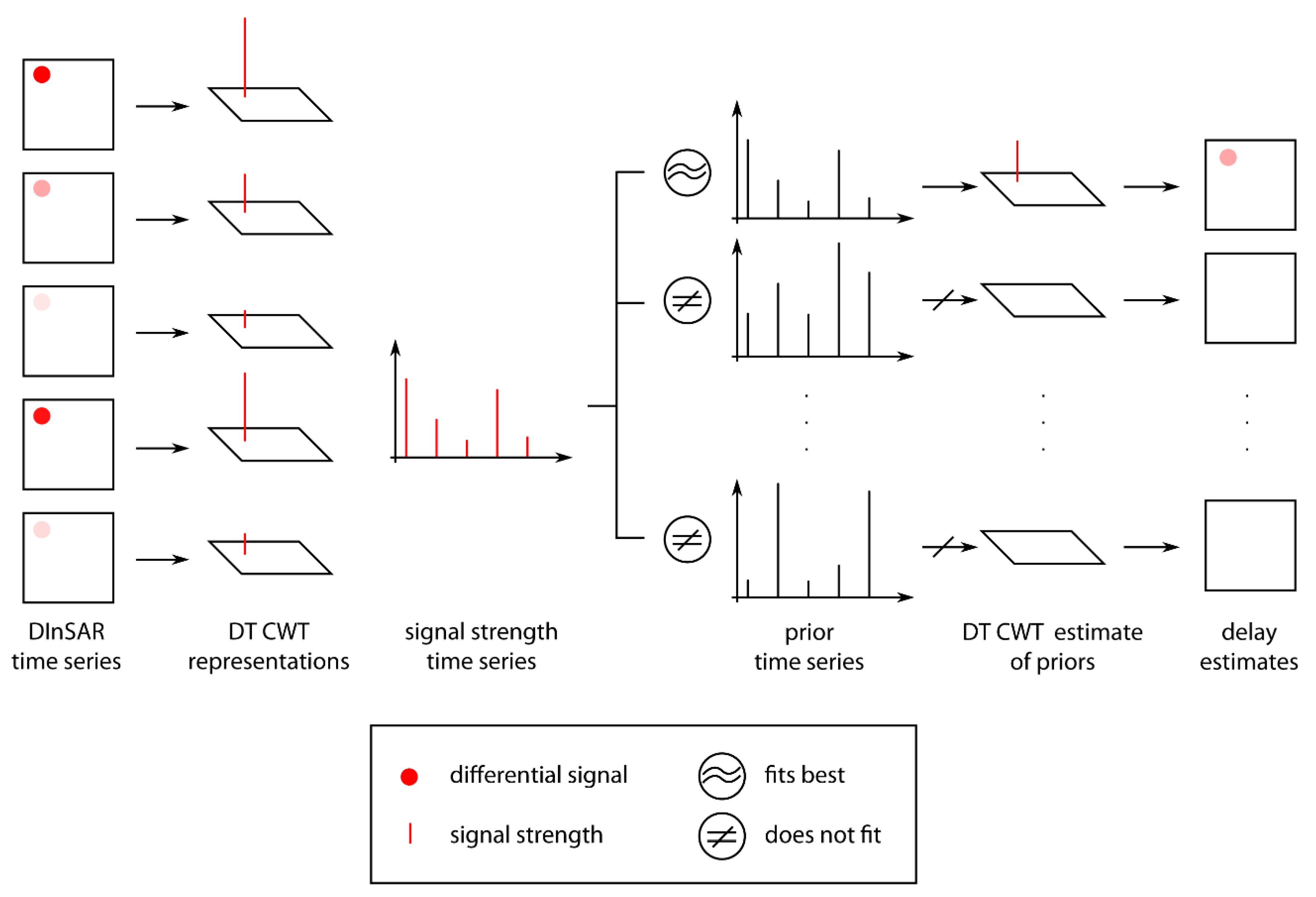
3.6. DInSAR Decomposition

To extract the gas plume related phase contribution from our interferograms, we used a wavelet-based DInSAR decomposition (WBDD) technique, which enabled us to integrate our estimates of the PWV contents in the volcanic gas plume into DInSAR analysis and thus allowed for the separate evaluation of gas plume related phase delays and their comparison with respect to all other phase contributions. The WBDD technique [63] was developed to deal with temporally unconnected DInSAR time series subsets and small stack sizes, and does not use the isotropy assumption to mitigate the atmospheric effect. The algorithm is based on Dual-tree complex wavelet transform ( D T - W T ), which is being used in a wide range of applications in the field of signal and image processing [64]. The D T - W T calculates the complex transform of a signal using two separate discrete wavelet transform decompositions (tree a and tree b), which may be regarded as equivalent to filtering the input signal with two separate banks of bandpass filters, that separately produce the real and imaginary coefficients of the complex wavelet. The D T - W T allows to capture both frequency and location information of a multidimensional signal, i.e., the times and locations at which these frequencies occur.
The WBDD technique requires at least two temporally interconnected interferograms as an input and the workflow is as follows (Figure 3). First, the D T - W T representations of all interferograms in the DInSAR time series are derived, i.e., complex wavelet coefficients are determined for each range azimuth position, where the phase of the coefficient determines the exact position of the wavelet in the interferogram and the modulus of the coefficient corresponds to the strength of the wavelet at given position. Second, each of these complex wavelet time series is analyzed using so-called priors, respectively prior time series containing information on the temporal evolution of any of the processes that possibly contributed to the total phase of the interferograms. That is, we are including prior information on the signal strength variations related to (i) inaccuracies of the DEM, (ii) linear deformation of the ground surface, and (iii) changing refractive properties of the ambient atmosphere and (iv) the volcanic gas plume (details on the determination and compilation of these priors are given in the following section). This prior information allows assigning each complex wavelet to their likely causes, depending on their best temporal correlation with the prior knowledge, and therefore enables to decompose the interferograms into signals related to the priors. The decomposition thus yields one separate radar propagation path delay estimate for each prior that was incorporated in the decomposition analysis of the DInSAR time series.

3.7. Priors Used for DInSAR Decomposition

To model the signal strength variations associated with different sources/processes affecting the interferometric measurements we used the following prior time series reflecting the temporal behavior of the corresponding processes. The dSWD time series, which were determined following the descriptions given in Section 3.4, were used as prior information for our algorithm, aiming to determine exclusively those interferometric phase variations, which are characterized by a similar temporal evolution as that of the PWV contents in the gas plume. As a result, we obtained the intersecting set of all gas plume related phase contributions contained in the DInSAR time series. Thus, our gas plume related phase delay estimates exclusively cover the area in which gas plumes of the different interferograms overlap.
The spatial and temporal baseline histories of the interferograms were included as prior information in order to capture small-scale topography related phase contributions, which were caused by errors in the DEM, and respectively by linear ground surface deformation. This works, because the effect of the DEM error typically evolves proportionally to the spatial baseline history of a DInSAR time series [65], and linear ground surface deformation evolves proportionally to the temporal baseline history. The values of the baseline histories were taken as they are and did not require any further computation, since these already represent differential values.
Furthermore, we estimated the refractivity related phase contributions of the ambient atmosphere in order to prevent them from leaking into the gas plume estimate, which involved incorporation of several priors in the analysis. In our approach we separately consider non-repeating phase contributions, which are caused by turbulent mixing of the atmosphere, and repeating phase contributions, which are rather related to the vertical stratification of the atmosphere and orographic effects, and thus typically correlate with the underlying topographic relief. Dirac-function priors were used to model APS spatial variation at each SAR acquisition, encompassing all non-recurrent phase contributions, which e.g., resulted from the turbulent transport of atmospheric and volcanic water vapor in the lower part of the troposphere, and thus were exclusively present at the times of single SAR observations. For this purpose one Dirac-function prior was included for each of the SAR scenes (using positive Dirac-functions for master scenes, and negative Dirac-functions for slave scenes), providing the benefit that no external information is required for this type of estimate, which in the following will be referred to as so-called single event APS estimate. In addition to single event APS estimation, we incorporated prior time series containing information on the differential temporal variations of relative humidity, surface temperature and surface pressure, which were derived from the detailed WRF simulation (described in Section 3.5) over a single spot on the summit of the volcano. This was done in order to also cover repeatedly occurring small-scale disturbances, which are related to stratification and to recurring formation of localized orographic clouds, and thus had not yet been captured by the single event APS estimates. Moreover, this approach decomposes the refractivity related propagation delay into different contributions of the single physical processes, which contribute to the variations of the tropospheric delay (compare with Equation (1) in Smith and Weintraub [66]), and thus enables us to separately examine the small-scale phase delay effects of the different physical processes in the troposphere.

4. Results

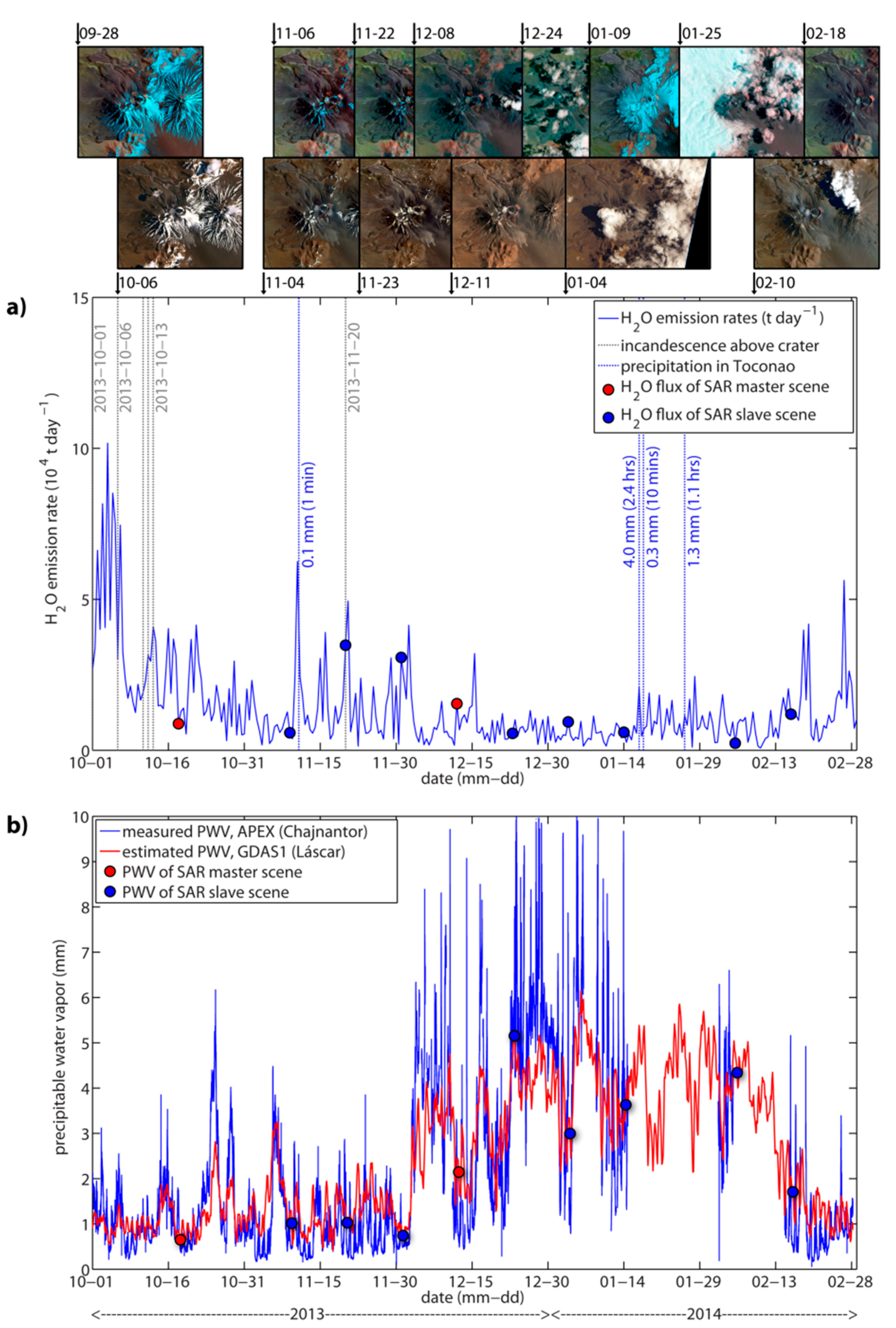
4.1. PWV Contents in the Volcanic Gas Plume of Láscar

During the days of the Multi-GAS survey in December 2012 and in the investigated period, the activity of Láscar volcano was characterized by quiescent degassing from the active crater (Figure 1). Webcam and visual on-site observations confirmed the frequent wind-blown dispersal of a white gas plume in south-easterly direction over the Puna plateau (Figure 1d). This gas plume therefore very often is also fully captured by the well-located scanning DOAS station. SO2 SCDs measured within the gas plume on the days with TerraSAR-X acquisitions ranged from 2.5 × 10¹⁶ to 2.8 × 10¹⁸ molecules·cm−2 and averaged at 7.2 × 10¹⁷ molecules·cm−2. SO2 SCDs exhibited diurnal variations, which were on average slightly enhanced during the early morning and evening hours.
The Multi-GAS measurements conducted during the field survey in December 2012 showed considerable fluctuations of the water contents at nearly constant CO2/S molar ratios, suggesting variable water loss due to condensation of water inside the cooling plume prior to the sampling by the instrument [33]. This in turn resulted in a particularly low average molar H2O/SO2 ratio of 9.37:1, as Multi-GAS instruments exclusively measure gaseous water vapor and do not take into account the LWC in the volcanic cloud. Using the values of Tamburello et al. [33] we thus determined a maximum molar H2O/SO2 ratio of 34:1, by means of which we finally arrived at a water content constituting roughly 90 mol.% of total gas emissions, which is in the range of typical values (85–99 mol.%) for high temperature gases from arc volcanoes elsewhere (e.g., Table 5 in Oppenheimer et al. [67]).
Our PWV estimates were thus obtained by conversion of SO2 SCDs at each scan angle of the plume cross sections using the fixed molar H2O/SO2 ratio of 34:1 (Figure 4a; see Appendix A for details). The amount of water vapor in the centerline of the plume was determined by finding the maximum PWV contents of each DOAS scan, and these were used to constrain the daily average PWV contents for days with TerraSAR-X acquisitions. Estimated daily average PWV contents obtained from the centerline of the plume ranged from 0.007 to 0.015 mm at the times of SAR observations (Figure 4b), translating to SWDs of 0.07 to 0.1 mm (Table 2, columns 3 and 8). Additionally, the average amount of water vapor in each DOAS scan was determined and used to calculate the daily average PWV contents of the bulk plume, i.e., by taking into account the whole plume cross sections at this time. Daily average bulk plume PWV contents ranged from 0.002 to 0.0035 mm (Figure 4b), corresponding to SWDs of 0.02 to 0.03 mm. Differential SWDs from the plume center were used as a prior time series (Table 3, column 3) for the estimation of the gas plume related phase contribution in the proximal portion of the gas plume. These values reflect H2O vapor contents at the crater rim, and are thus not representative for PWV contents arriving at the scanning plane of the scanning DOAS (Figure 2a), since they do not take into account downwind evaporation.
Potential evaporation rates were thus determined for the measurement periods of the scanning DOAS (Figure 4c; see Appendix B for details on evaporation calculation), and used to upscale the H2O/SO2 ratio, which was thereby adjusted to increase proportionally to evaporation rates, which in turn strongly depend on wind speeds (Figure 4d) over arid areas. The resulting variable ratio was then used to upscale the SO2 SCDs at each scan angle of the plume cross sections as described above (and in Appendix A), at this time, however, taking into account the effect of downwind evaporation (Figure 4e).
We assume that such adjusted estimates provide a more reasonable approximation of the temporal variations in PWV encountered above various points of the plume cross sections. Estimated daily average PWV contents obtained from the centerline of the plume ranged from 0.8 to 9.6 mm at the times of SAR observations (Figure 4f), translating to SWDs of 6.4 to 77.0 mm (Table 2, columns 4 and 9). Daily average bulk plume PWV contents ranged from 0.2 to 2.5 mm (Figure 4f), which correspond to SWDs of 1.6 to 20 mm (Table 2, columns 5 and 10). The daily average bulk plume PWV contents were used for the determination of the second dSWD prior time series (Table 3, column 4), which in turn was used for the estimation of the gas plume related phase contribution in the distal portion of the volcanic gas plume.

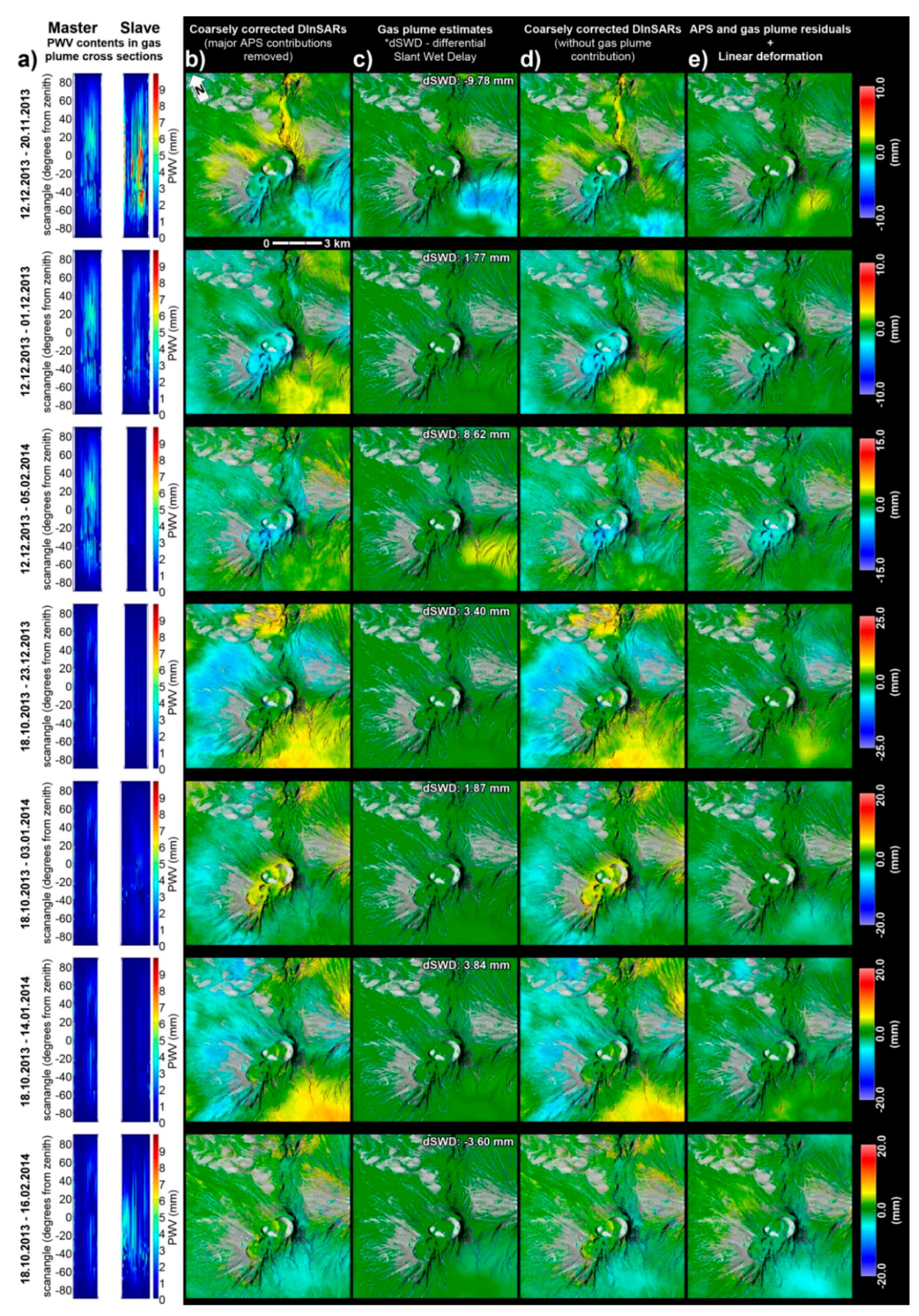
4.2. Gas Plume Related Phase Delays

PWV contents obtained for the distal portion of the volcanic gas plume (Figure 5a) were used to exemplify how the DInSAR decomposition analysis can be used to map the corresponding refractivity anomalies in the DInSAR time series. To this end, we used the entire DInSAR data set described in Section 3.3, and applied all priors listed in Section 3.7. The differential interferograms, which were coarsely corrected according to the steps described in Section 3.5, show a relatively large amount of coherent pixels (Figure 5b). Pronounced phase changes are visible around the summit and on the flanks of the volcano, representing the sum of phase contributions from individual sources including slow and linear ground surface deformation [40], residual topography due to errors in the DEM, and refractivity fluctuations in atmosphere and volcanic gas plume.
The coarsely corrected DInSARs were decomposed (Section 3.6) in order to obtain the intersecting set of repeating gas plume related phase contributions, which are present in all interferograms of the analyzed DInSAR time series. Owing to the different temporal development of PWV contents which were determined for the two different sections of the plume (Figure 4b,f), we accordingly retrieved two contrasting phase delay results for the ascending part of the plume above the crater (Figure 6a) and the downwind portion of the gas plume (Figure 6b). The phase delay map obtained for the prior time series of the gas plume related SWDs above the crater rim (Table 3, column 3) displays a weak altitude correlated shortening of the delay over an area which is largely confined to the summit region of the volcano (Figure 6a). The phase delay map obtained for the downwind portion of the gas plume (Figure 6b) in contrast shows a lenticular pattern that indicates lengthening of the radar propagation path over an area that agrees well with the most common eastward plume transport directions observed during spring and late summer of that period (see Appendix A, Figure A1c,d).
DInSAR decomposition further yielded phase delay maps for each of the other priors that were included in the analysis. A detailed description of these maps (which are displayed in Figure 6 and Figure A4) would however go beyond the scope of this paper and thus can be found in the Appendix E and Appendix F.

4.3. Isolation of the Gas Plume Related Signal in DInSARs

The phase delay map obtained for the downwind portion of the gas plume (Figure 6b) was used to determine the gas plume related phase contributions in each DInSAR image of the time series. For this purpose the theoretical dSWDs, which were used as a prior for this estimate (Table 3, column 4), were multiplied by the respective phase delay estimate, which resulted in simple phase difference maps depicting the repeating gas plume related phase contribution present in each of the DInSAR maps (Figure 5c). The phase difference maps use the same scale bounds as those used in Figure 5b in order to display the relative effect of the gas plume related phase delay on the interferometric measurements with respect to other phase contributions. Each of these maps reveals a lenticular phase difference pattern, which equals the pattern that was already observed in the corresponding phase delay map (Figure 6b), and which persists throughout the entire DInSAR time series. As a consequence of the mathematical operation used to retrieve these maps, the amplitude of the pattern varies in proportion to the a-priori constraints on the differences in gas plume PWV content and is most pronounced in those DInSARs, in which the differential PWV contents determined for the epochs of master and slave SAR acquisitions were the highest (compare Figure 5a,c). Moreover, it is interesting to note that the contrast between plume related and atmospheric signals was more pronounced in the DInSAR images of subset 01.
As a next step, the gas plume related phase difference maps depicted in Figure 5c were subtracted from the coarsely corrected DInSAR maps depicted in Figure 5b in order to mitigate the gas plume related phase contribution. The resulting DInSAR maps (Figure 5d) differ clearly from the coarsely corrected DInSAR maps, which still contain the gas plume related signal. As expected, the removal of the gas plume related signal is most obvious in the DInSARs of subset 01, where the mitigation in two cases (DInSARs 1 and 3) even resulted in a change to the opposite delay direction over the area which was affected by the gas plume (Figure 5d, rows 1 and 3).

4.4. Residuals of the Refractivity Related Phase Delay and Ground Deformation

To verify the efficiency of our decomposition analysis, we now examine the residual phase, which persists when all estimated refractivity and DEM error related phase contributions have been removed from the DInSAR maps. To this end, the complete set of refractivity and DEM error related phase delay estimates obtained from WBDD analysis as shown in Figure 6 and Figure A4 (and further detailed in Section 4.2 and Section 5.3 and the Appendix) were multiplied with the values of their respective input prior time series to obtain phase difference maps corresponding to each of the DInSARs. Similarly the single event APS estimates of individual SAR acquisitions (Figure A4) were combined to form phase difference maps for each interferogram by subtraction of the slave APS from the master APS. The resulting phase difference maps were then subtracted from the coarsely corrected DInSARs (Figure 5b) obtaining interferograms, which mainly contain the residual phase and topographic contributions attributed to a deforming ground surface (Figure 5e). This refined correction more or less efficiently removed small-scale phase delay patterns, which were caused by the volcanic gas plume and a turbulent atmosphere, as well as small-scale DEM errors related to acquisition geometry, respectively spatial baseline, leaving only some faint and blurry signatures of low amplitude.
In between the blurry residuals of non-deformation related phase contributions a putative small-scale ground deformation signal can be observed in the central of the three north-eastern summit craters of Láscar. The signature occurs in each of the DInSARs, and indicates a progressively subsiding crater floor confined to an arcuate fault, where Pavez et al. [39] detected co-eruptive subsidence of the crater floor during the 1995 eruption, and where Richter et al. [40] identified linear subsidence during the period 2012–2016.

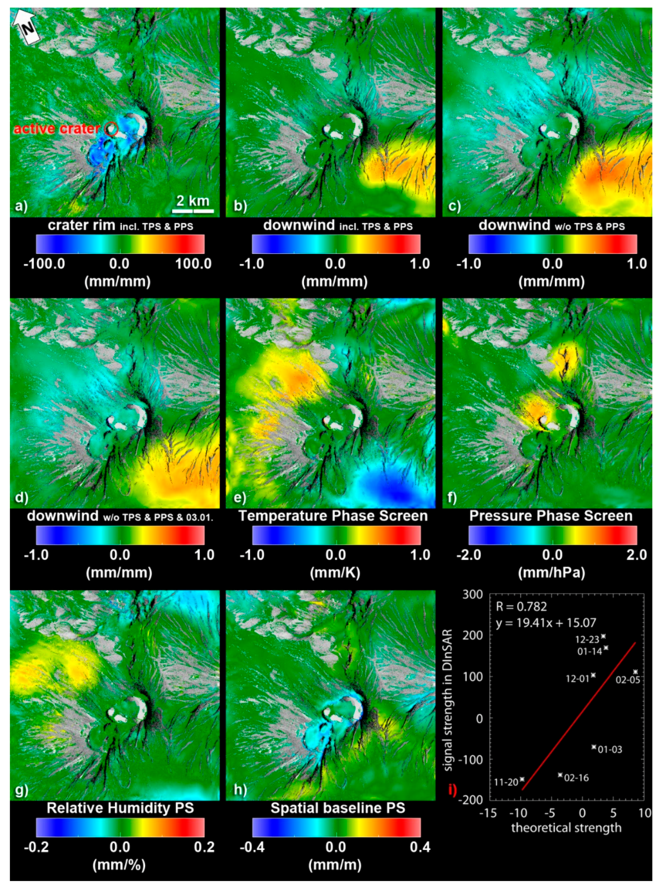
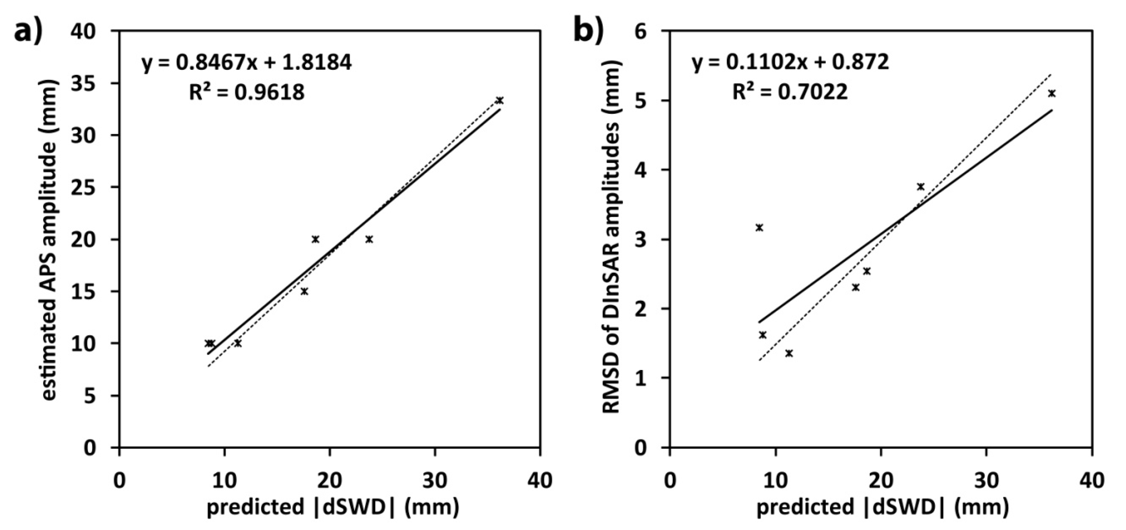
4.5. Validation of the Gas Plume Signal Estimate

The phase delay estimates which were obtained by decomposition analysis can be validated by means of relating the position and strength of the estimated DInSAR signal to the input prior information. We thus compared the signal strength of the lens-shaped gas plume pattern in each of the DInSAR maps (Figure 5b) to the strength of the theoretical dSWDs (Table 3, column 4), which served as a prior for the corresponding gas plume estimate (Figure 6b). For this purpose the signal strength S of the gas plume related phase contribution was determined for each interferogram using the amplitude of the gas plume pattern in the phase delay estimate obtained for the downwind portion of the plume (orange color in Figure 6b) by means of following Equation (3).
S = s g n ( X · Y )   | X · Y |
here s g n denotes the sign function and X · Y = i X i Y i is the dot product of vectors X and Y , where X corresponds to the amplitude of the gas plume estimate obtained from WBDD and Y is the associated measured signal in each of the DInSARs, which were used in the analysis. The comparison revealed a moderate positive linear relationship between signal strength S and theoretical strength (Table 3, column 4), which is fairly well represented by the regression line depicted in Figure 6i, since 61% (R2 = 0.61) of the total variation in measured signal strength can be explained by the linear relationship between theoretical strength and signal strength. Thus, in principle, this regression line can be used to determine the gas plume related phase delays even of those DInSARs for which no corresponding ground-based gas emission measurements are available.

5. Discussion

5.1. Why the Distinction between Periods of Volcano Deformation and Enhanced Degassing is Important

This work constitutes the first serious attempt to quantify gas plume related phase delays in differential interferometric radar measurements of a persistently degassing and deforming volcano. We propose a method that enables us to attain gas plume detection by means of satellite-based radar interferometry and demonstrate that gas plume related phase delays in DInSARs can be isolated and mapped, if a-priori constraints on the gas plume PWV contents obtained from independent gas measurements are included in the analysis of DInSAR data.
The distinction between periods of local volcano deformation and enhanced degassing can be of vital importance both for early warning purposes and for a better understanding of volcano-tectonic processes. Degassing and deforming volcanoes often display a variety of deformation sources, which reflect the complex interplay between (i) magma emplacement/retreat, (ii) accumulation/discharge of volcanic gases and (iii) changes in hydrothermal activity, as e.g., was observed at Campi Flegrei in Italy [68,69], or at Lastarria in Northern Chile [70]. Retention and loss of magmatic and hydrothermal volatiles play a central role in virtually any of the processes that lead to volcano deformation. Gas emission measurements on deforming volcanoes thus provide essential auxiliary information on the ultimate cause of individual deformation observations [71,72], and deformation measurements likewise may deliver explanations for observed changes in the amount and composition of gas emissions [73].

5.2. How Methodological Limitations Can be Turned into Benefit

Area-wide precise ground deformation measurements by means of InSAR require adequate mitigation of atmospheric phase contributions, which may be challenging in small SAR datasets. In particular, repeatedly occurring spatially correlated errors, which e.g., may be caused by orographic clouds and volcanic gas plumes, are difficult to remove [74,75]. Insufficient resolution of meteorological and DEMs used for correction of DInSAR data adds further uncertainties to retrievals of ground deformation. Moreover, most modern SAR satellites revolve Earth on a sun-synchronous dusk-dawn orbit, and record their data along the day-night boundary, i.e., at a time, when emission rates of continuously degassing volcanoes typically are the highest [76,77,78], which in turn increases the risk of having disturbances due to volcanic water vapor emissions in InSAR measurements. Such noise may, however, be transformed into data, as soon as phase contributions of different sources can be distinguished, which can be accomplished by integration of a-priori constraints.
In our approach we derive prior constraints of volcanic H2O emissions using measurement techniques, which are commonly used in volcano monitoring, hence providing the benefit of data availability for a comparatively large number of volcanoes. Volcano monitoring generally demands rapid response, in order to assess the volcanic hazard in a timely manner, and the specific information which would be relevant to identify more rapid ground deformations often may be confined to a limited number of available SAR observations. Therefore it seems highly desirable to develop a method that allows removing disturbances of any kind even from small sets of interferograms, where conventional methods as persistent scatterer interferometry and the small baseline subset algorithm would fail. The presented method addresses the problems of the different measurement methods mentioned above, and exploits the fact that DInSAR analysis allows for mapping of water vapor distribution.
In the following subsections, we will discuss the phase delay effects that can be observed in the phase delay maps which were obtained for the proximal and distal sections of the plume, and relate our observations to variations in gas emission rates. Furthermore, we will examine the relative and absolute effects of these phase delays with respect to (seasonal) variations in water vapor contents of the ambient atmosphere. Finally, we will assess the benefits and drawbacks associated with our approach.

5.3. Phase Delay Effects above the Crater and Downwind of Láscar

We now elucidate the contrasting phase delay effects that are observed in the phase delay estimates obtained for the proximal and distal portions of the gas plume (Figure 6a,b).
The phase delay map determined for the downwind portion of the gas plume (Figure 6b) shows a lenticular pattern that indicates lengthening of the radar propagation path due to enhanced moisture over an area that agrees well with the most common eastward plume transport directions observed during spring and late summer of that period (see Appendix D, Figure A1c,d). Westward drifting plumes, which generally may have occurred during early summer (see Appendix D, Figure A1c,d and Figure A2), did obviously not occur at times of the SAR acquisitions we used to obtain our gas plume related phase delay estimates, as these would have prohibited detection of a repeatedly occurring phase delay pattern. Moreover, such westward drifting plumes would less likely leave any repeating traces in the SAR signal, due to a less pronounced humidity/refractivity contrast between plume and surrounding atmosphere in early summer. This is further supported by the fact that easterly winds over the Atacama region typically have a lower velocity (see Appendix D, Figure A2), and tend to be less stable with respect to their direction (see Appendix D, Figure A1c,d), resulting in unsteady plume transport directions, which additionally impedes formation of pronounced repeating patterns. Wind speeds were generally larger during periods with eastward plume transport (spring and late summer; see Appendix D, Figure A1a and Figure A2), causing plume transport to be more turbulent, and thus the volcanic plume was very likely less condensed, and instead contained more vapor during that period.
Additional phase delay estimates of the distal portion of the gas plume were processed without (Figure 6c,d) additionally including prior information on the temporal behavior of surface temperature and pressure in order to show the effect of APS mitigation by the corresponding temperature and pressure phase screens (Figure 6e,f). For the computation of the estimate displayed in Figure 6d we furthermore reduced the number of input DInSARs omitting the interferogram that was formed from SAR acquisitions of 18 October 2013 and 03 January 2014 (Figure 5, row 5). Prior information on relative humidity variations were included in all of the mentioned cases, yielding a relative humidity related phase delay estimate (Figure 6g), which was mitigated from all other phase delay estimates. Comparison of the resulting gas plume phase delay estimates clearly shows that the repeating patterns of the gas plume signal (Figure 6c,d) can readily be reduced (Figure 6b), when a surface temperature and air pressure correction (Figure 6e,f) is included in the WBDD analysis. The gas plume related phase delay estimate depicted in Figure 6b thus clearly represents the result in which the separation of gas plume related phase delays from other phase contributions was most successful.
The phase delay map obtained for the prior time series of the gas plume related SWDs above the crater rim (Table 3, column 3) shows a weak altitude correlated shortening of the delay over an area which is largely confined to the summit region of the volcano (Figure 6a). The location of this phase delay signature is thus consistent with the assumption that the dSWDs, which were used as a prior for this estimate (Table 3, column 3), are representative for the temporal evolution of SAR signal strength variations measured above the crater. The observed shortening of the delay, however, contradicts the hypothesis that this signature can be ascribed to enhanced moisture over the respective area, since a water vapor field would produce a lengthening of the delay (compare Equation (1) in Smith and Weintraub [66]). Furthermore, the phase delay patterns in this estimate strongly resemble the patterns observed in the DEM error related phase delay estimate (Figure 6h), which was obtained using the temporal history of the spatial baseline (Table 3, column 8), suggesting that the phase delays, that the algorithm attributed to the gas plume above the crater, are in fact rather related to errors in the DEM (detailed in Appendix F). This suspicion is further substantiated, if one compares the shape of the two corresponding priors, which strongly resemble each other in appearance. As a consequence of this similarity, the signal obviously was assigned to both priors by the WBDD algorithm, since this signal does not perfectly match to any of the priors. This phase delay estimate thus is a good example for a case in which the algorithm failed to isolate possible gas plume related phase delays from other phase contributions. Thus, care must be taken to avoid misinterpretation of model results.

5.4. Gas Emission Rates from Láscar Volcano

Gas emission rates from Láscar volcano were determined and compared to our PWV estimates (Figure 4b,f), in order to illustrate how much water vapor has been emitted from the volcano to produce the corresponding PWV contents in the gas plume, and to relate our observations to variations in volcanic degassing activity. SO2 emission rates were calculated from scanning DOAS measurements using wind field information obtained from GDAS1 soundings provided in the web-based archive of the National Oceanic and Atmospheric Administration’s (NOAA) Air Resources Laboratory [79]. These were then upscaled by the H2O/SO2 molar ratio of 34:1 obtained from Multi-GAS, in order to retrieve the corresponding H2O-fluxes (Figure 7a).
Assuming a constant H2O/SO2 ratio and a constantly strong condensation of the emitted water vapor, the H2O (SO2) emission rates ranged from 5 to 100 kt·day−1 (150 to 2900 t·day−1) and averaged at 12 kt·day−1 (350 t·day−1) during the considered period. Based on these assumptions we estimate that the total errors of our upscaled H2O emission rates likely were around −15 to +45% and thus even more skewed towards underestimation than the error envelopes of corresponding SO2-fluxes, which were constrained to about −10 to +30% (see e.g., [80] for error determination). Gas emission rates of October and November 2013 showed more pronounced variations and were on average slightly enhanced (about 19 kilotons of H2O and respectively 550 tons of SO2 per day) with respect to the rest of the period (10 kilotons of H2O and respectively 300 tons of SO2 per day). The enhanced degassing activity of October and November further was accompanied by elevated heat dissipation from the main active crater as was suggested by intermittent night-time webcam observations of illuminated gas plumes (obtained on several days during the first half of October and lastly on 20 November 2013; see Figure 7a), which indicated the presence of incandescent material inside the active crater [81]. Such observations support the repeated influx of fresh magma from depth feeding the high-temperature gas exhalations at the surface of the crater bottom, thus suggesting a concurrent increase of magmatic gas emissions and progressive drying of the ambient hydrothermal system (e.g., [41]), which may have altered gas ratios temporarily. Contemporaneous measurements of SO2 emission rates confirmed this suspicion and appropriately showed sharp increases over the course of each of these days (Figure 7a).
Bearing these observations in mind, we compared the gas emission rates with the estimated PWV contents of the gas plume (Figure 4b,f) revealing that gas emission rates evolved differently than the PWV contents obtained for the gas plume above the crater (Figure 4b), but displayed a very similar temporal evolution as that of the PWV contents, which were obtained for the downwind portion of the gas plume (Figure 4f). The latter thus likewise were enhanced during the period of increased volcanic activity.

5.5. Estimation of Background Atmospheric PWV Contents

Atmospheric disturbances due to volcanic gas plumes are intuitively expected to be more pronounced during periods which are characterized by strong variations of gas emission rates and low ambient atmospheric humidity. Determination of PWV contents in the local atmosphere was thus done to be able to approach the relative and absolute effects of the plume on the specific SAR acquisitions. In the Atacama region the driest conditions are typically found during the period late March to early December, and between local midnight and 11:00 a.m. [82]. Background PWV contents in the atmosphere above the volcano were retrieved from vertical atmospheric GDAS1 profiles provided by NOAA (see Appendix C for equations). These estimates were also cross-checked with PWV estimates obtained from radiometer measurements (Figure 7b) provided by the Atacama Pathfinder EXperiment (APEX), which is located about 30 km north of Láscar at a very similar altitude of 5100 m above sea level (m.a.s.l.), thus reflecting similar weather conditions.
Because PWV is a measure of how much water is available for potential rainfall, it dictates precipitation intensity, which thus reversely can be used to infer accompanying PWV. To give an impression of when to expect enhanced PWV contents and to further complete the picture of the hydrological cycle of the study area, we will first briefly describe the characteristic seasonal patterns according to which precipitation typically occurs at Láscar, and narrow down the periods during which precipitation actually was encountered in the course of the observation interval of our case-study.
The considered period covers parts of the “dry season”, which is characterized by dry and cold prevailing westerly synoptic winds, and is spanning most of the year (here October, November and second half of February are included), as well as the “wet season” ranging from December to February, which is characterized by less stable atmospheric conditions, resulting in more humidity being transported to the Andes by frequently recurrent warm easterly winds [83]. As a consequence of this easterly moisture source, precipitation on the leeward slopes of the Puna plateau exhibits a marked seasonality in particular at elevations below 3500 m.a.s.l., where about 90% of the annual precipitation (<20 mm·year−1) falls during the (austral) summer months, that is from December to March [84]. The associated rainfall events typically are very short, but can become quite intense. During the considered period, a weather station (operated by the Instituto de Investigaciónes Agropecuarias) located at 2500 m.a.s.l. in Toconao, a small village roughly 30 km NW of Láscar, recorded 4 events of precipitation which amounted to a total of 5.7 mm (equivalent to liters per square meter) within only 3.6 h (vertical blue lines in Figure 7a). At elevations above 3500 m.a.s.l. the situation is slightly different and precipitation (<200 mm·year−1) occurs even during the dry winter period, mostly in the form of snow with the greatest snowfall frequency happening to occur near the Tropic of Capricorn [85], where also Láscar coincidentally is located. Láscar volcano thus commonly is almost completely (except for the hot bottom of the currently active crater) covered with several meters of snow during the “dry season”, which however melt and sublimate due to the warm winds of the “wet season”. Such snowmelt events hence constitute an important source for groundwater recharge, which potentially affect the hydrothermal activity of Láscar. The temporal development of the snow and cloud cover encountered at Láscar during the period of our case-study is illustrated by a sequence of satellite images (Aster, Landsat-8, and EO-1 ALI) in the top panel of Figure 7a in order to give a visual impression of the situation associated with different epochs of the temporal development of atmospheric moisture.
Measured and estimated atmospheric PWV contents were at average below 1 mm during October and November 2013, sharply increased to 5 mm in December 2013, stayed enhanced through the first half of February 2014, and finally decreased again to 1 mm in the second half of February 2014 (see Figure 7b and also Table 2, column 6). The comparatively low PWV values determined for the times of SAR observations used in this work reflect the pronounced atmospheric transparency around sunrise, and the resulting SWDs (Table 2, column 11) are in good agreement (R2 = 0.96; see Appendix G for detailed statistics) with the amplitudes of associated phase delays observed in the corresponding DInSARs (Figure 5b and Figure A4).
It is interesting to note that the apparent SO2 (H2O) emission rates generally were particularly low whenever the ambient atmospheric water vapor levels were elevated, which is clearly visible especially during the “wet season” (compare Figure 7a,b). This observation suggests the presence of low hanging clouds beneath the volcanic gas plume, which may have caused attenuation of the absorption signal due to contributions of scattered light that did not pass through the plume [86]. Moreover, a fraction of the degassing SO2 may have been scrubbed by dissolution into the aqueous phase e.g., during possible events of fresh water influx into the hydrothermal system [87], though this would most likely only have a marginal effect on the emissions of the hot degassing dome of Láscar, which is less probably being deeply infiltrated by permeating waters that interact with ascending magmatic fluids, than the peripheral low-temperature vent sites. Another mechanism, which may be considered to explain the observed diminution of SO2-fluxes is the dissolution of emitted SO2 in the water droplets of low hanging clouds [88], which, however, usually is not particularly effective over a short distance, and the associated scavenging rate of SO2 emissions is generally estimated being on the order of merely a few percent of total emitted SO2 per hour. This in turn leads to relatively long atmospheric lifetimes of SO2 emissions, which were shown to range between several hours to days according to weather conditions [89].
Estimated PWV contents inside the volcanic gas plume (Figure 4b,f) and modeled atmospheric PWV contents outside the plume (Figure 7b) were compared in order to assess the humidity/refractivity contrast between ambient atmosphere and volcanic plume. The comparison revealed that PWV contents at the downwind plume centerline (0.8 to 9.6 mm) were generally larger than the PWV contents of the ambient air (<1 mm) during periods with dry atmospheric conditions, i.e., most of the year. During early summer the situation was different, and the downwind plume PWV content (<1 mm) was less contrasting with respect to the PWV content of the atmospheric background (2–5 mm). PWV contents of the downwind bulk volcanic plume (0.2 to 2.5 mm) were accordingly much less contrasting most of the year when compared to background atmosphere, and were slightly higher than ambient atmospheric humidity only during the first three SAR observations of the time series (on 18 October 2013, 20 November 2013, and 01 December 2013). Future studies exploiting a larger InSAR dataset of Láscar might therefore well capture these seasonalities in gas plume and atmospheric PWV contents, the latter of which were already identified at Láscar [39] but also elsewhere, e.g., at Campi Flegrei and Vesuvius [90]. PWV contents determined for the proximal part of the plume above the crater rim were in general negligible with respect to PWV contents of the ambient atmosphere (0.007 to 0.015 mm on the centerline of the plume, and 0.002 to 0.0035 mm averaged over the bulk plume).
The corresponding SWDs obtained for the proximal part of the plume above the crater rim ranged from 0.07 to 0.1 mm in the centerline of the plume (Table 2, column 8) and from 0.02 to 0.03 mm in the bulk plume and thus were negligible compared to the InSAR accuracy. The SWDs in the more distal part of the plume downwind of the crater, however, were on the order of background atmospheric SWDs (5.3 to 41.5 mm; compare with Table 2, column 11), and ranged from 1.6 to 20 mm in the bulk volcanic plume and from 6.4 to 77.0 mm along the plume centerline (Table 2, columns 9 and 10), which is more than large enough to produce a detectable effect in interferometric measurements, as can be seen in the corresponding phase delay maps (Figure 5c).
Our results thus collectively suggest that refractivity changes in volcanic gas plumes may, particularly under dry climatic conditions, have a significant effect on DInSAR measurements, hence requiring extreme caution, when alleged deformation signals are detected above or downwind of visibly degassing volcanoes, especially if these are located at high elevations.

5.6. Limitations of the Proposed Method

Our approach was hampered by several practical limitations, which were mainly related to spatial data coverage and temporal coincidence of the different measurement techniques that we combined.
Simultaneous measurements of Multi-GAS and DOAS instruments were unfortunately not available for the period considered for DInSAR analysis, and thus our PWV estimates had to rely on the gas concentration measurements obtained during a short Multi-GAS survey conducted about one year prior to the period considered here. This is of particular relevance, since Láscar exhibited elevated SO2 emission rates and incandescence during the first two months of this period, suggesting a slightly enhanced magmatic activity, which likely was accompanied by temporarily altered gas ratios. At the same time, the snow cover on the summit of the volcano was observed to be reducing strongly (satellite images in Figure 7), which may be an indication for concurrent fresh water influx into the peripheral hydrothermal system. Thus, there is evidence for both, elevated emissions of magmatic SO2 and increased hydrothermal H2O contributions of meteoric origin. The assumption that molar H2O/SO2 ratios stayed more or less constant throughout the entire period of our case study therefore may not be perfectly appropriate. Availability of data from a stationary Multi-GAS instrument certainly would have helped to better characterize the temporal variations of molar H2O/SO2 ratios, and thus to better quantify the water vapor contents at the instance of gas sampling by the Multi-GAS.
Moreover, volcanic gas plumes typically contain variable amounts of condensed liquid water in addition to gaseous water, which are not taken into account by the measurements of Multi-GAS instruments, and thus unequivocally lead to an underestimation of the water vapor contents, which are expected to increase in the downwind portion of the volcanic gas plume due to evaporation. Such an underestimation could be avoided, if water vapor contents were mapped in situ across the whole extent of the gas plume, e.g., by means of airborne gas composition measurements, though this approach would not be very practicable but rather labor and cost-intensive in the view of satellite revisit times of 11 days.
Additionally, the DOAS measurements are generally restricted to daylight conditions and thus deviate from SAR acquisition times by up to 2 h (Figure 2b). Due to this deviation in acquisition times and because the proposed DInSAR decomposition analysis requires only one representative PWV value for each SAR image (see Section 3.6 and Section 3.7), we thus used daily average gas plume PWV contents, in order to determine the SWD that such PWV contents theoretically would produce in the LOS of a SAR image. In the view of strong diurnal degassing variations, which are characterized by pronounced gas emission maxima around sunrise and sunset [77,78], such time averaged values however inevitably lead to systematic underestimation of the water content in the volcanic plume at the times of the SAR observations.
Furthermore, our analyses have shown that different locations within the gas plume may exhibit a different temporal evolution of the PWV contents, which may appropriately be captured by inclusion of corresponding priors. However, we point out that modeling the evolution of water vapor contents over the entire extent of the gas plume even by means of two prior time series still is a simplification. Prudent sampling of the gas emission data in time and space hence constitutes an important prerequisite in order to obtain a-priori information, which yields feasible results from DInSAR decomposition analysis.
This becomes particularly clear, if one notes that the position of the plume center varied during the measurement period, because the gas plume of Láscar somewhat meanders within the scan range of the scanning DOAS. Transport of the plume changed between north-easterly and south-easterly directions approximately every 10 min, which roughly corresponds to the duration of 1 complete DOAS scan. This resulted in different plume positions in consecutive scans, which is why the sequences of consecutive scans in Figure 4a,e have a corrugated appearance. We thus assume that the resulting daily average plume center statistic may not be representative for the effect that the bulk plume has on SAR measurements further downwind of the volcano, since the gas distribution along plume cross sections is highly irregular when the plume meanders. For this reason, we chose to use the PWV contents of the bulk gas plume instead of those from the plume center in order to estimate related phase delay in the downwind portion of the gas plume.
Further limitations of our approach lie within the applicability of the WBDD technique. The method makes extensive use of ancillary data, which have to be made available to obtain reasonable results. To successfully isolate the plume-induced signal from total phase, it is necessary to additionally include the priors of all potentially interfering signals in the analysis, i.e., the temporal and spatial baseline histories, which were used as priors for the estimation of phase delays related to DEM error and linear deformation, as well as several priors defining the atmospheric phase delay of each acquisition. We consider that, even when all required priors are being used, the estimated gas plume related signal still may additionally contain phase information related to any other interferometric signal that coincidently correlates with the gas plume related signal (as was shown in Section 5.3 for the phase delay estimates depicted in Figure 6a,h). In the presence of a non-linearly deforming ground surface it may additionally be necessary to include prior information on the temporal behavior of the associated deformation signal, which e.g., could be derived from deformation measurements of independent ground-based methods, such as GPS, or tiltmeters. Last, but not least, the DInSAR decomposition analysis exclusively yields reasonable results for the gas plume estimate when there is significant overlap between gas plumes of different SAR acquisitions, since “solitary” plumes would be captured by the single event APS estimates causing a gap in the temporal evolution of the repeating pattern. To capture the whole gas plume at the times of SAR acquisitions instead of only the intersecting area of multiple different gas plumes definitely would have been an asset.

5.7. Advantages of the Proposed Method

The WBDD technique provides a framework for data fusion, enabling to integrate a variety of external information, such as weather data, results from gas emission monitoring or even independent deformation measurements into the analysis of DInSAR time series. These time series may be very short and it is shown that the combination of only three SAR acquisitions already enables us to generate high-quality DInSARs including estimates of their corresponding phase screens (as demonstrated in Appendix H). The algorithm does not require any information on the location of the plume, in order to find the related “disturbance” in the interferometric signal. This is of particular advantage to the application described here, since we lack precise information on the heading of the plume at the times of SAR observations, apart from a rough approximation that can be derived from webcam images and wind directions offered by the weather models. Also, no information about the interferometric signal strength, rather merely the shape of the prior time series is used, because prior information about the relations between signal strength and amplitudes of the prior time series is allotted by chance, which is why the prior information can be scaled arbitrarily without influencing the location of the associated filtered phase delay patterns. Correspondingly, the radar path delay estimates can be validated by the position and strength of the estimated signal in relation to the corresponding prior information (Section 4.5). The gas plume is transported by advection, therefore has a direction, and is correspondingly anisotropic. For this reason, the WBDD technique arguably is the best choice for the detection of gas plumes in interferometric measurements. Additionally, the ability to use temporally unconnected time series subsets enables to use only those DInSARs which have a very small spatial baseline. This helps avoid unwrapping errors due to erroneous DEMs.

6. Summary and Conclusions

Here, we presented a novel time-space-based filtering method that allows for the isolation and mitigation of virtually any conceivable non-intrinsic error source that affects interferometric ground deformation measurements, by means of including prior constraints on their temporal behavior in the DInSAR analysis. Including prior information on gas plume related refractivity variations furthermore enabled us to identify and map spatially correlated repeating interferometric phase delay patterns caused by refractivity changes within volcanic gas plumes that were drifted in a similar direction during several subsequent SAR acquisitions. Apart from potentially being a new tool to detect volcanic gas plumes in DInSAR data, the WBDD algorithm thus provides the possibility to mitigate the plume-induced phase delay, where deformation measurements are the main purpose of monitoring.
Similarly to the small baseline subset algorithm our technique operates on a pixel-by-pixel basis on areas that show sufficient coherence throughout the entire DInSAR time series. The algorithm requires only a relatively short time series comprising at least 2 temporally interconnected DInSARs, respectively 3 observations in order to capture the plume related phase delay, and when more than 2 interferograms are available, these do not necessarily have to be temporally connected. Moreover, the method allows for iterative determination of PWV contents in the volcanic gas plume by matching the estimated phase delays with theoretical phase delays derived from ground-based gas emission measurements, which resulted in reasonably realistic values for the gas plume of Láscar volcano.
To our knowledge this is the first time that phase delay effects in volcanic water vapor emissions were quantitatively investigated by means of radar interferometry. Examination of PWV contents and associated phase delay effects in the volcanic gas plume of Láscar yielded daily average bulk plume PWV contents of 0.2 to 2.5 mm water column, which would generate plume wide excess path delays in the range of 1.6 to 20 mm. The corresponding H2O emission rates ranged from 5 to 100 kt·day−1 and remarkably displayed a similar temporal behavior as the PWV contents that were obtained for the downwind portion of the gas plume. Our observations consider that the locations of the interferometric patterns in the phase delay estimates are consistent with determined locations of the volcanic plume, and variations in phase delay amplitudes are in good agreement with variations in the strength of the emission source and humidity of the ambient atmosphere. Therefore there is ample evidence, that the DInSAR phase variations detected by the WBDD algorithm are indeed related to refractivity variations in the volcanic plume. Additional independent data on plume location and chemistry at the time of SAR acquisitions would help to further corroborate our results as a proof of concept.
We have illustrated that integrating a-priori information from gas emission measurements and meteorological data into the analysis of DInSAR time series provides previously unknown possibilities to efficiently decompose the radar signal into different phase contributions. The implications of this new technique are wide, ranging from improved deformation measurements to simultaneous quantification of volcanic outgassing activity, DEM error estimation, and meteorological applications, such as mapping and quantification of turbulently transported atmospheric PWV in each SAR acquisition. Our results furthermore encourage the use of data from ground-based gas emission monitoring networks, such as NOVAC for calibration and validation of satellite-based measurements on active volcanoes.

Author Contributions

Conceptualization, S.B. and F.-G.U.; Methodology, S.B. and F.-G.U.; Software, F.-G.U.; Validation, F.-G.U. and S.B.; Formal Analysis, F.-G.U. and S.B.; Investigation, S.B. and F.-G.U.; Data Curation, S.B. and F.-G.U.; Writing-Original Draft Preparation, S.B., F.-G.U., T.H.H. and T.R.W.; Writing-Review & Editing, S.B., T.H.H., T.R.W., and F.-G.U.; Visualization, S.B. and F.-G.U.; Supervision, T.R.W. and T.H.H.; Project Administration, T.R.W. and T.H.H.; Funding Acquisition, T.R.W. and T.H.H.

Funding

This project was funded by the Helmholtz Association through the “Remote Sensing and Earth System Dynamics Alliance”, which was realized in the framework of the Initiative and Networking Fund, and by the GEOMAR Helmholtz-Centre for Ocean Research Kiel (project-id: HA-310/IV010). This is a contribution to VOLCAPSE, a research project funded by the European Research Council under the European Union’s H2020 Programme/ERC consolidator grant no. ERC-CoG 646858.

Acknowledgments

The authors would like to thank Claudia Bucarey from Observatorio Volcanológico De los Andes del Sur (OVDAS) for installation and maintenance of the permanent scanning DOAS instrument at Láscar volcano, providing an invaluable gas emission data set. TerraSAR-X High Resolution Spotlight scenes were provided by DLR and were tasked and acquired by the proposal WA1642. Further acknowledged is the Atacama Pathfinder EXperiment for providing archived weather and radiometer data, and the Instituto de Investigaciónes Agropecuarias for providing the precipitation data of their weather station in Toconao on the server of the Dirección Meteorológica de Chile (Meteochile). The Aster, Landsat-8 and EO-1 ALI images used in this study are made available by the U.S. Geological Survey through the USGS EarthExplorer platform (https://earthexplorer.usgs.gov/). Michael Eineder is thanked for fruitful discussions and encouragements regarding the work on this paper. Martin Zimmer, Christian Kujawa, Elske de Zeeuw-van Dalfsen, Nicole Richter, Mehdi Nikkho, Jacky Salzer, Giancarlo Tamburello, and Ayleen Gaete for joint field work activities and discussions. The editors and anonymous reviewers are thanked for their comments that helped improving the manuscript.

Conflicts of Interest

The authors declare no conflict of interest.

Appendix A. Estimation of PWV Contents in the Volcanic Cloud

Water vapor contents in the volcanic plume were estimated by scaling the SO2 column density profiles measured by our scanning DOAS with the molar H2O/SO2 ratio derived from gas compositional measurements of the Multi-GAS instrument. For this purpose we used the ‘raw’ differential SO2 SCD output of the NOVAC-software [91], which in our case provides SO2 path length concentrations in units of ppm·m, that is SO2 concentration distributed along the effective light paths captured at each observing angle of the scans. Several conversions of the ‘raw’ data were necessary, in order to estimate the precipitable water vapor content of the volcanic cloud in a vertical atmospheric column right above each point of the plume cross-sections.
The light paths associated with the conical viewing geometry of the scanning DOAS instrument are generally inclined with respect to the vertical, entailing amplification of the absorption signal in relation to the signal that would be obtained along the more direct zenith light path due to extension of the distance that the incoming light has to travel through the absorbing air mass. Extension of the effective light path along inclined viewing directions is typically taken into account by means of the so-called air mass factor (AMF), which relates the measured SO2 SCDs to their respective vertical column densities (VCDs). The SO2 VCDs thus simply correspond to the ratio of SO2 SCDs and air mass factor as expressed in Equation (A1) (e.g., [92]).
S O 2   V C D   ( p p m · m ) = S O 2   S C D A M F G
Here, we used a geometrical approximation of the air mass factor A M F G , that can be derived for each viewing direction of a scan by means of Equation (A2) [91]
A M F G = ( c o s ( β )   c o s ( δ )   + s i n ( β )   c o s ( θ )   s i n ( δ ) ) 2 + ( s i n ( β )   s i n ( θ ) ) 2 ( c o s ( β )   s i n ( δ ) +   s i n ( β )   c o s ( θ )   c o s ( δ ) ) 2   + 1 ,
where θ is the scan angle (or zenith angle, which corresponds to the angle between observing elevation and zenith position), δ = 0 is the tilt of the scanner of our DOAS station at Láscar, and β = 60 is half the opening angle of the conical scanning surface. More sophisticated radiative transfer corrections were not performed additionally. The resulting SO2 VCDs are given as path length concentrations in units of ppm·m, and were used to approximate the corresponding PWV contents in units of mm water column. This required several steps of conversion, which were combined in Equation (A3).
P W V   ( m m ) = 10   m m × S O 2   V C D ( p p m · m ) × 2.5 × 10 15 S O 2   m o l e c u l e s · c m 2 × H 2 O / S O 2 3.34 × 10 22 H 2 O   m o l e c u l e s · c m 2
Single steps of this conversion equation were derived from the following relationships. A path length concentration of 1   p p m · m   S O 2 roughly corresponds to a column density of 2.5 × 10 15 S O 2   m o l e c u l e s · c m 2 at standard conditions for temperature and pressure, that is 298.15 K and 1 atmosphere air pressure (e.g., [91]). The corresponding number of vertically integrated water vapor molecules per square centimeter thus is readily obtained by scaling the SO2 VCDs in units of molecules·cm−2 with the H2O/SO2 molar ratio determined from the Multi-GAS measurements. H2O VCDs in units of molecules·cm−2 further can be converted to the total amount of water vapor present in a vertical atmospheric column, also known as column integrated water vapor (IWV), which is commonly stated as the vertically integrated mass of water vapor per unit area (e.g., kg·m−2). At conditions of 1 atmosphere air pressure and 273.15 K one can find that an IWV of 1   g   H 2 O   c m 2   ( =   10   k g   H 2 O   m 2 ) roughly corresponds to a column density of 6.02214 × 10 23   m o l e c u l e s · m o l 1 / 18.015   g · m o l 1 = 3.34 × 10 22   H 2 O   m o l e c u l e s · c m 2 , and respectively to 10   m m of an equivalent column of liquid water (A4) (pp.3 and 4 of the Appendix in McClatchey et al. [93]; or p.3 in Wagner et al. [94]).
3.34 × 10 22 H 2 O   m o l e c u l e s · c m 2 = 1   g · c m 2 = 10   k g · m 2 10   m m   w a t e r   c o l u m n
Conversion of IWV in units of kg·m−2 to PWV in units of mm water column is obtained using Equation (A5) (e.g., [61])
P W V ( m m ) = I W V ρ L W ,
where the density of liquid water ρ L W typically roughly is equal to 1   g · c m 3 , and thus a water vapor column density of 1   k g · m 2 roughly corresponds to 1   m m height of an equivalent column of liquid water.

Appendix B. Compensation of Downwind Evaporation

LWCs in the plume above the crater rim were unknown, thus it was not possible to determine the actual evaporation rate from a predefined amount of liquid water. Considering increasing water vapor concentrations, respectively increasing H2O/SO2 ratios in the downwind portion of the volcanic plume, we thus calculated the drying power of the ambient air, respectively potential evaporation rates at plume height, based on climatic variables obtained from GDAS1 soundings, and terrain surface roughness. Potential evaporation rates were then used to scale our fixed H2O/SO2 ratio in order to compensate for downwind evaporation.
Potential evaporation rates correspond to the amount of liquid water that can be transformed to vapor through evaporation, if sufficient water is available (e.g., [95]). Assuming an unlimited availability of water, evaporation can in such a situation continue until the air above the evaporating surface approaches saturation humidity, and therefore actual evaporation cannot exceed potential evaporation. In the present case, availability of liquid water does not seem to be a limiting factor inside the plume, since we made the observation that the plume typically still is partly condensed when it arrives at the scanning DOAS. We thus assume that scaling by the potential evaporation rate yields a feasible approximation of the increase in water vapor at the expense of liquid water in the downwind portion of the volcanic cloud. We further assume that downwind dilution of water vapor due to dispersion of the plume is largely covered by the variations of the SO2 column densities measured by the DOAS, since both water vapor and SO2 are equally affected by diffusion and turbulent mixing processes (e.g., [96]). The amount of evaporation occurring inside the plume is largely controlled by the humidity of the entrained ambient air and the degree of turbulent mixing with air parcels of the plume, which is mainly governed by wind speed and atmospheric stability. Evaporation is thus commonly more pronounced during periods with dry atmospheric conditions and high wind velocities, which cause the transport of the plume to be more turbulent, and it is less significant, when the atmosphere is more humid and less turbulent, due to small transport velocities.
Evaporation rates were calculated by an aerodynamic (respectively mass-transfer) method (e.g., [97]), using temperatures, dew point temperatures, and wind speeds obtained from GDAS1 soundings provided by the National Oceanic and Atmospheric Administration (NOAA) [79]. The aerodynamic approach can be expressed by a Dalton-type Equation (A6) [98,99],
E P   ( c m · s e c 1 ) = f ( u ) ( e s e ) ,
in which E P is the rate of potential evaporation (cm·sec−1), f ( u ) is a wind speed function (cm·sec−1·hPa−1), respectively the vapor transfer coefficient, which is based on a logarithmic vertical wind velocity profile, and the second term ( e s e ) is the humidity term corresponding to the vapor pressure deficit of air (hPa). The product of both is typically referred to as the drying power of air. The wind function of the Dalton-type equation can be written as (A7) (Equation (4) in [100])
f ( u )   ( c m · s e c 1 · h P a 1 ) = ρ A I R   ϵ k 2 ρ L W   P   u 1   l n ( z 1 / z 0 ) 2 ,
where ρ A I R and ρ L W correspond to the density of moist air and liquid water (g·cm−3), respectively. ϵ = 0.622 is the ratio of the molar mass of water vapor ( 18.015   g · m o l 1 ) to the average molar mass of dry air ( 28.9647   g · m o l 1 ), and k = 0.4 is the dimensionless von Kármán’s constant describing the logarithmic velocity profile of a turbulent air flow near a rough boundary with a no-slip condition [101], i.e., it is assumed that wind speed is zero directly above the surface. u 1 refers to the wind speed (cm·sec−1) at measurement height z 1 (cm above ground surface), and P is barometric pressure (mbar or hPa) at measurement height z 1 . z 0 is the surface roughness height (cm above surface), which corresponds to the average height of obstacles in the trajectory of the wind [102]. The density of moist air ρ A I R (g·cm−3) was calculated using the ideal gas law (A8)
ρ A I R   ( g · c m 3 ) = 0.1 P R d ( 1 + 0.608 q v ) ( T + 273.15 ) ,
where R d   ( J · k g 1 · K 1 ) = 287.04 is the gas constant for dry air, P is barometric pressure (hPa), T air temperature (°C), and q v specific humidity (g·g−1), which in turn was approximated by Equation (A9).
q v   ( g · g 1 ) = ϵ e P
Here, ϵ = 0.622 again is the ratio of the molar mass of water vapor to the average molar mass of dry air, e is the partial pressure of water vapor in hPa, and P is barometric pressure in hPa.
Saturation vapor pressure e s (hPa) was calculated using the August–Roche–Magnus formula (A10) [103] with coefficients determined by Sonntag [104] (Table 1 in [105]).
e s   ( h P a ) =   6.112 e x p   17.62 T 243.12 + T ,
where T is temperature in Celsius degree. Water vapor partial pressure e (hPa) was calculated as a function of relative humidity and saturation vapor pressure using Equation (A11)
e   ( h P a ) = R H 100 e s ,
where R H / 100 is the fractional relative humidity, and e s saturation vapor pressure at the ground level of the GDAS1 sounding. Relative humidity (%) was obtained by comparison of actual water vapor partial pressure e and saturation vapor pressure e s , using Equation (A12) with coefficients determined by Alduchov and Eskridge [105].
R H   ( % ) = 100 e e s =   100 e x p ( 17.625 T D ) / ( 243.04 + T D )   e x p ( 17.625 T ) / ( 243.04 + T ) ,
where T and T D are air temperatures, and respectively dew point temperatures in Celsius degree. Density of liquid water ρ L W (kg·m−3) was calculated from temperatures T (°C) at plume height using Equation (A13) that was empirically determined by Jones and Harris [106].
ρ L W   ( k g · m 3 ) = 999.85308 + 6.32693 × 10 2   T 8.523829 × 10 3   T 2 6.943248 × 10 5 T 3 3.821216 × 10 7 T 4
The roughness height z 0 was approximated by Equation (A14), which was experimentally determined by Plate and Quraishi [107] in wind tunnel experiments, and which yields fair results in the absence of more precise information [108].
z 0   ( c m ) = 0.15 h ,
where h is the average height of roughness elements (cm). As in this work the volcano is the main obstacle, and since the evaporating surface, respectively the volcanic plume typically is located roughly at summit altitude of the volcano, the average height of roughness elements relevant for the turbulent mixing of the plume with the atmosphere, was assumed to be equal to the height of the volcano above the surrounding plateau (about 750 m).

Appendix C. Estimation of PWV Contents in the Atmosphere

Background PWV contents in the atmosphere above the volcano were approximated by means of an empirically determined regression Equation (A15), which is based on the experimental results of Garrison and Adler [109] and proved to be applicable over a broad range of climatic conditions (e.g., [110]). The calculation requires climatic variables including pressure, dew point temperature and temperature, which were obtained from vertical atmospheric GDAS1 profiles provided by NOAA.
P W V ( m m ) = 4.1173   R H   P 1013.25 ( 273.15 + T ) e s + 0.2 ,
where R H is relative humidity (%), which was calculated using Equation (A12), P is barometric pressure in hPa, T is temperature in Celsius degree, and e s saturation vapor pressure at the ground level of the GDAS1 sounding was calculated using Equation (A10). Note that we reduced the intercept of the equation from +2 to +0.2 mm water column, in order to adapt the formula to hyper-arid conditions that are characterized by average PWV contents of less than 1 mm.

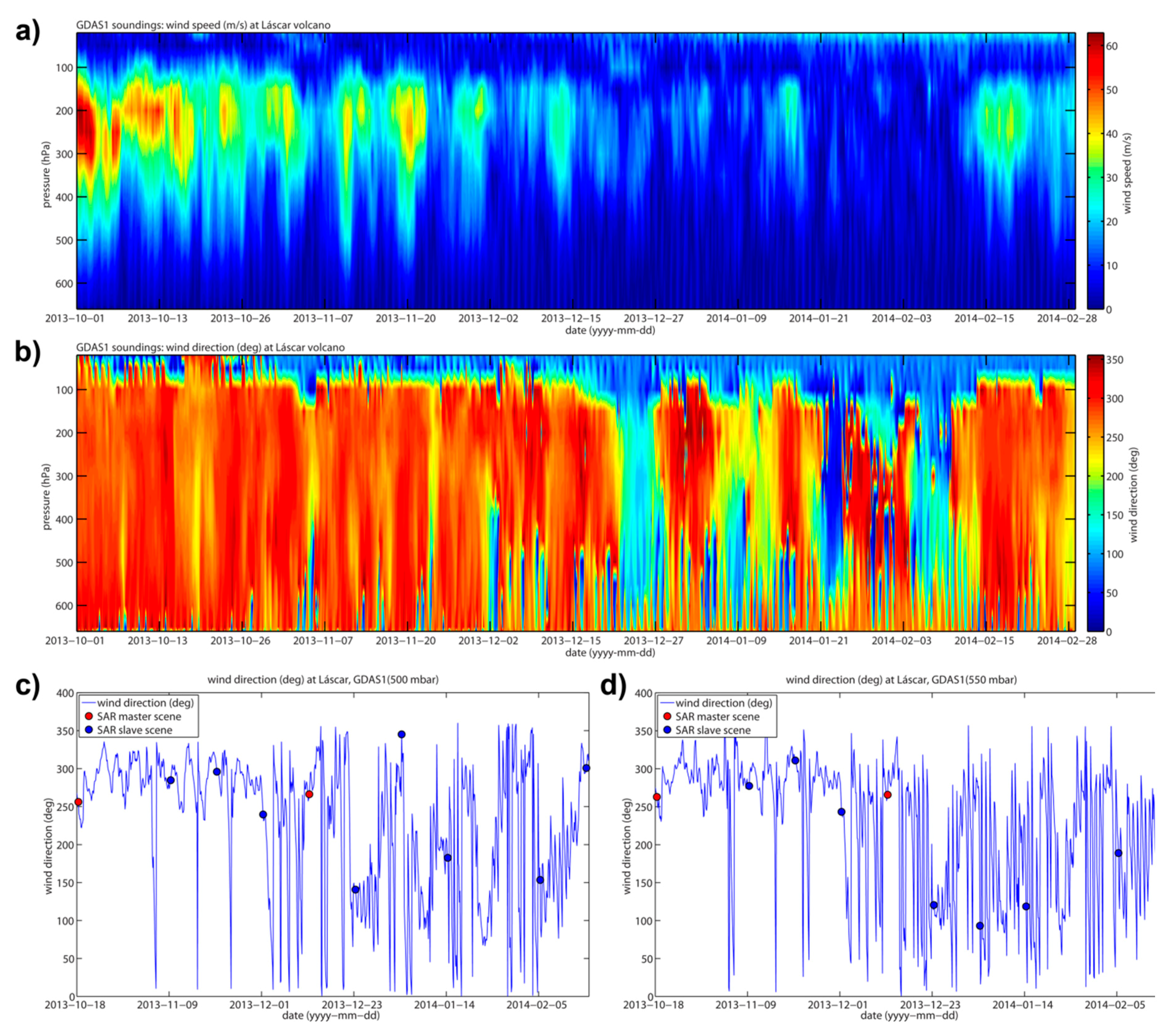
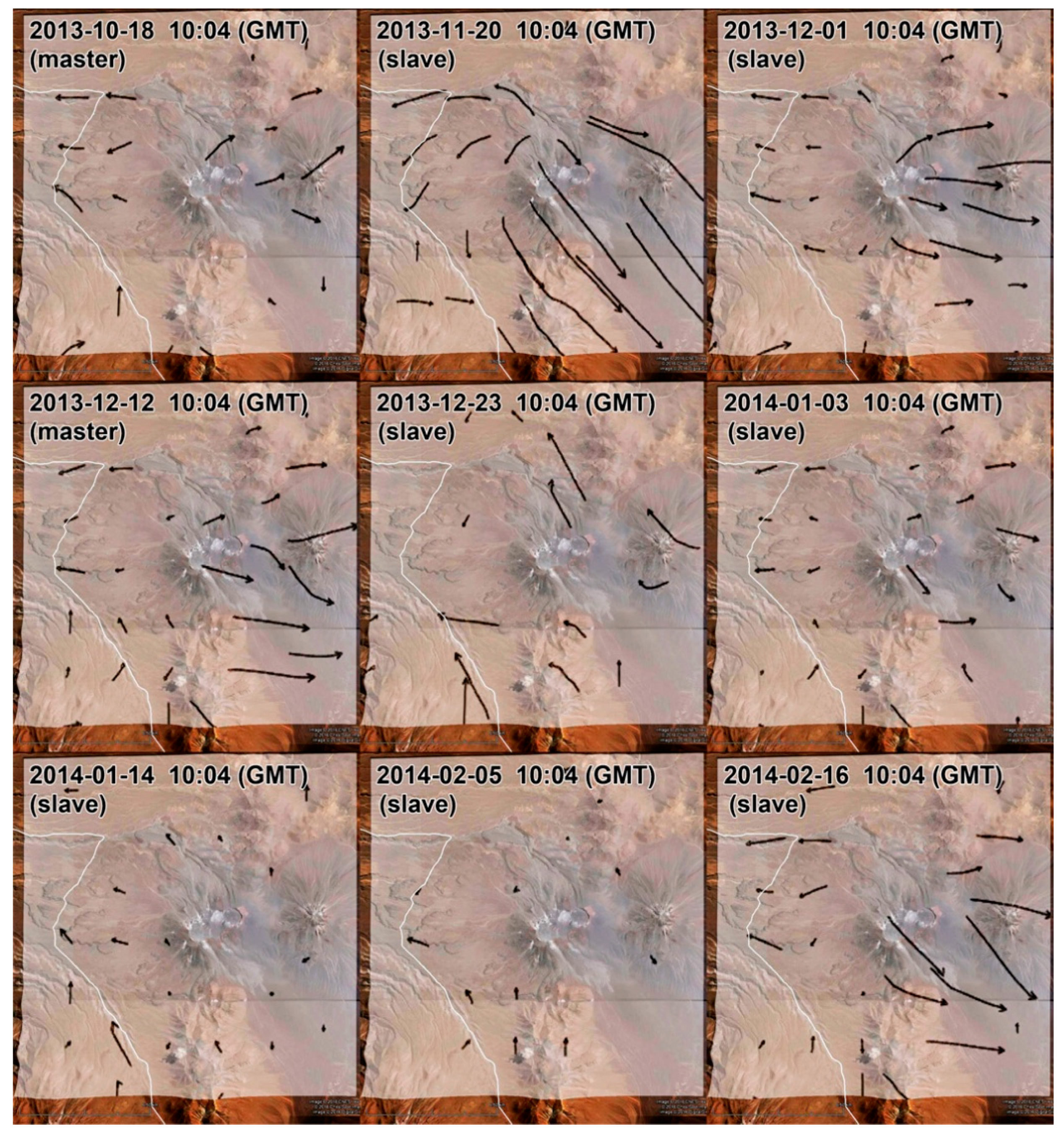
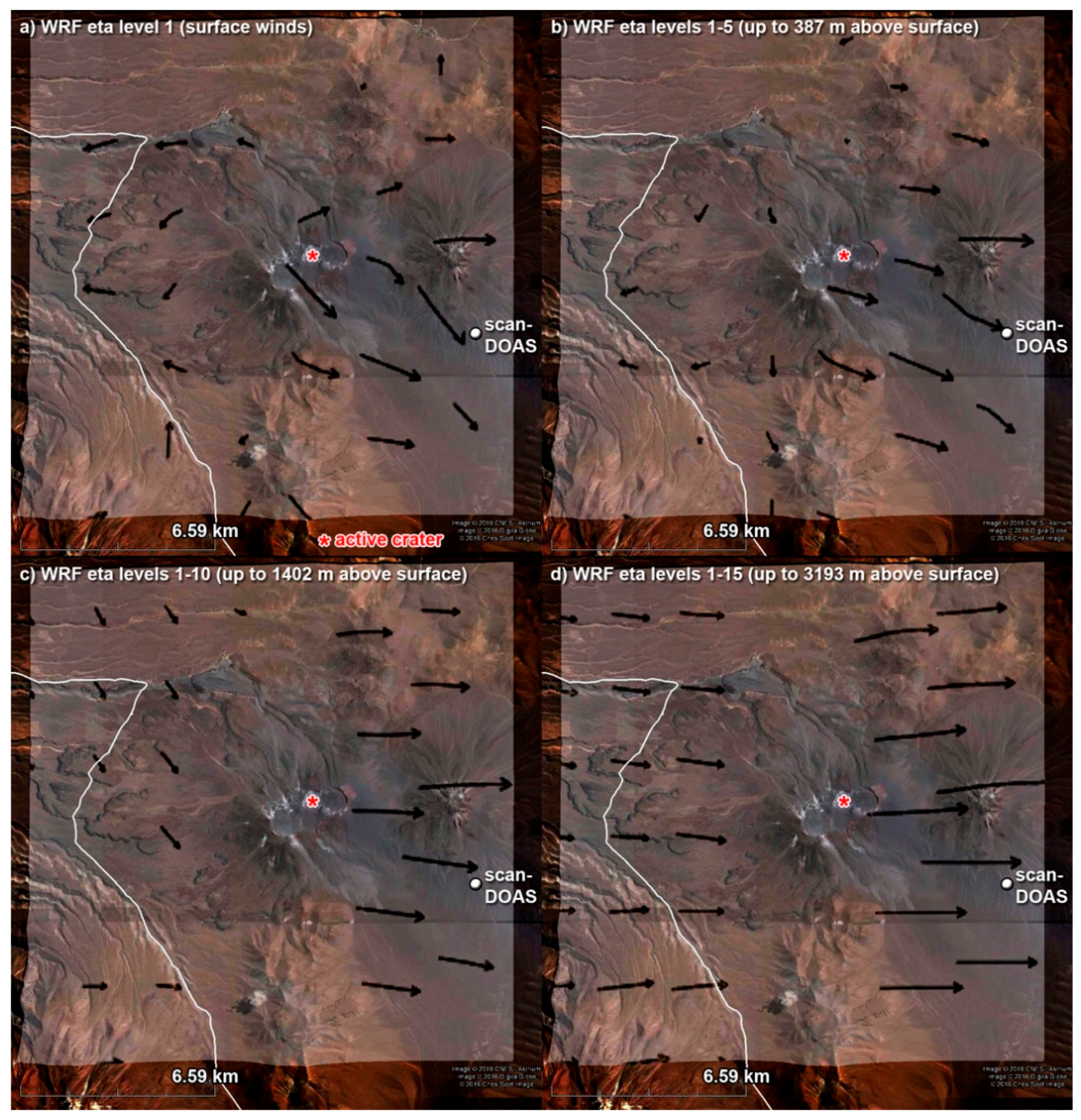
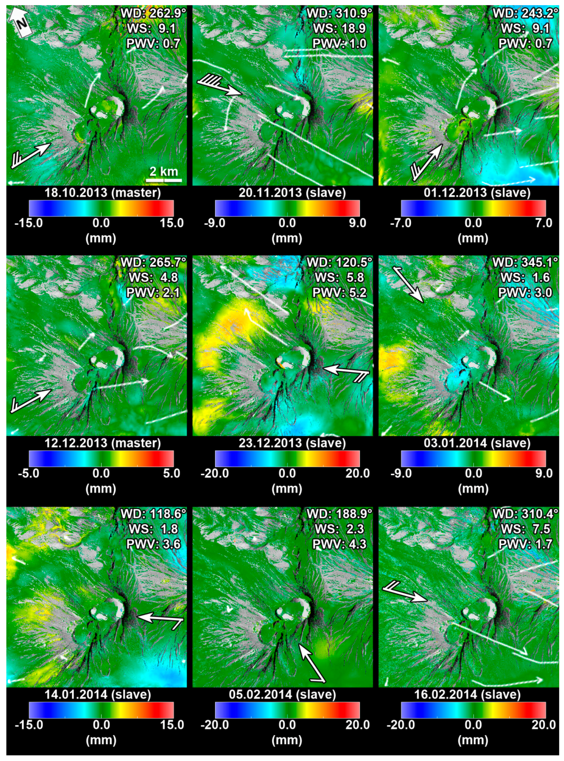
Appendix D. Wind Field during SAR Acquisitions

Wind, in particular over arid regions, plays a major role for the transport of humidity in the atmosphere, which is also true for the humidity emitted from volcanoes. In order to understand humidity variations in the atmosphere above a volcano, it is thus necessary to know about the local wind field. The temporal variations of the wind field above Láscar volcano were examined using atmospheric soundings of the Global Data Assimilation System (GDAS1) with one-degree grid spacing provided by NOAA. The soundings were concatenated to form a time series of wind speed and direction encountered at Láscar volcano during the period of interest (Figure A1a,b). Wind speeds at plume altitude ranged from 0.1 to 18 m·sec−1 during the period of interest, and generally decreased throughout the whole atmospheric profile during austral summer (December to February) (Figure A1a). High altitude winds over the region usually are prevailing westerly throughout the year (orange colors in the upper part of Figure A1b), and are interrupted by short periods, which are dominated by easterly wind anomalies during austral summer. Surface winds typically are oriented according to topography, and exhibit pronounced diurnal variations (alternating blue and orange colors in the lower part of Figure A1b). These diurnal variations are characterized by valley winds (anabatic upslope breezes depicted by orange colors in the lower part of Figure A1b) that typically occur during daytime due to insolation of mountain flanks, and increasing wind speeds towards the evening (light blue colors in the lower part of Figure A1a), whereas rather calm mountain winds (katabatic downslope breezes and over-hill flows) prevail during the night (depicted by blue colors in the lower part of Figure A1b and dark blue colors in Figure A1a). Diurnal variations in surface wind directions are more prominent during summer, frequently resulting in a characteristic diurnal pattern of plume transport directions. We observed that in the morning hours of a summer day the plume typically drifts towards west or northwest, turning over south towards east before noon, where it stays more or less steady until sunset. Downslope winds frequently force the plume to follow the steep morphology of the volcano.
Time series of wind directions in the range of typical plume heights, namely several 100 m above and below the summit of Láscar volcano were extracted from the 500 and 550 mbar pressure levels of the GDAS1 soundings, respectively, in order to narrow down the range of possible plume transport directions at the times of SAR acquisitions (Figure A1c,d). Wind directions at the time of SAR acquisitions of track 111, which were conducted around sunrise at about 10:00 a.m. UTC (Figure 2b), were predominantly westerly during spring 2013 and late summer 2014, whereas easterly directions prevailed during early summer 2013. Wind directions were generally very similar over the broad altitude range of both pressure levels, indicating relatively stable wind conditions. Pronounced differences in wind directions above and below summit were mainly observed during early summer, when winds tended to be less stable with respect to the direction, and were characterized by low velocities.
Figure A1. (a,b) Time series of vertical atmospheric profiles depicting variations in (a) wind speed and (b) wind direction. Note the weak winds accompanied by strong variations of wind directions during austral summer (ranging from December 2013 to February 2014). (c,d) Time series of wind directions some 100 m (c) above and (d) below the summit of Láscar (500 and 550 mbar pressure levels of the GDAS1 soundings, respectively). Wind directions at the time of SAR observations are indicated by red (master scene) and blue dots (slave scene). Wind directions during austral summer (ranging from December 2013 to February 2014) were predominantly easterly at the time of SAR observations.
Remotesensing 10 01514 g0a1
We further complemented our observations by means of an additional high resolution wind field analysis, which is based on 3-dimensional gridded hindcasts of the Weather Research and Forecasting model (WRF). This we did, in order to resolve how the wind field evolved from turbulent flow close to the ground surface to laminar flow at higher altitude during the times of SAR acquisitions, because the gas plume typically is being emitted at the interface between surface flows and higher altitude flows. To this end, the WRF simulation was run using a 900 m horizontal grid spacing and a vertical division of 51 (terrain-following) eta levels.
Surface wind fields obtained from the lowest eta level of the WRF simulation, reveal that katabatic (downslope) winds prevailed during most SAR acquisition times (Figure A2).
Figure A2. Time series of surface wind fields obtained from the lowest eta level of WRF, determined for acquisition times of each SAR image. Katabatic (downslope) mountain winds prevail at the time of SAR acquisitions, which were recorded during the early morning hours at about 10:04 a.m. (UTC), respectively 07:04 a.m. (CLST).
Remotesensing 10 01514 g0a2
The wind fields of all acquisition times were averaged, in order to match the cumulative SAR delay estimates produced by WBDD. This was done for the first eta level, which represents the wind conditions closest to the surface (Figure A3a). Changing conditions with increasing altitude were captured by means of gradually increasing the number of eta levels, which were included into the averaged wind field. In other words eta levels 1–5, 1–10, and 1–15 were combined to yield averaged wind fields (Figure A3b–d). Average wind direction of the terrain following winds close to the surface was predominantly towards southeast aloft the plateau, and heading downslope, which is mainly oriented towards west, over the western flank of the plateau (Figure A3a). Gradual integration of more eta levels into the average wind field nicely illustrates the turning direction of the winds with increasing altitude (Figure A3a–d), finally arriving at upper tropospheric westerly trade wind directions, which are typical for this region (Figure A3d).
Figure A3. Averaged wind fields combining wind fields of all SAR observation times. (a) Average surface winds from eta level 1 (b) Average winds up to 387 m above surface (c) Average winds up to 1402 m above surface (d) Average winds up to 3193 m above surface.
Remotesensing 10 01514 g0a3

Appendix E. The Decomposed APS: Non-Repeating and Repeating Atmospheric Phase Delays

E.1. Single Event APS Estimates

Delay maps of single event APSs were generated to mitigate non-repeating atmospheric disturbances from the gas plume estimate, and were used to infer the meteorological conditions during each SAR observation (Figure A4). These APS estimates are presented in the form of simple phase delay maps, where the scale indicates lengthening or shortening of the radar delay in units of millimeters. Such phase delay maps are snapshots of the meteorological situation, reflecting the spatial distribution of water vapor fields at the times of SAR acquisitions. Atmospheric disturbances aloft volcanoes are generally more pronounced and show more complex flow patterns on the lee side of the volcanic edifice [18]. This anisotropic distribution of turbulent atmospheric patterns can be attributed to the presence of volcanic gas plumes on the one hand, but also to orographic effects that govern the transport of moist air over mountainous terrain [17,20]. Orographic effects comprise diabatic heating of air masses over insolated mountain flanks and orographic lifting of air masses that are pushed by the wind, causing upslope advection of moist air that is forced to rise following the steep topography, and to cool adiabatically causing an increase of the relative humidity.
Figure A4. Single event APS estimates superimposed by surface wind fields obtained from the lowest eta level of WRF (thin white arrows). Scales indicate range change in millimeters, and are unique to each image, in order to enhance contrast by depicting the full range of each image. Katabatic (downslope) mountain winds prevail at the time of SAR acquisitions recorded during the early morning hours (10:04 a.m. GMT, local time is offset −3 h). Wind barbs indicate wind directions and wind speeds above the summit of Láscar volcano, which were obtained from GFS hindcasts at the times of SAR acquisitions. The barbs are displaced upstream in order not to cover the delay signatures of the summit area. The individual lines of the barbs represent the wind speeds in units of knots (half strokes correspond to 5 knots and full strokes correspond to 10 knots). Wind directions (clockwise degrees from North), wind speed (m·sec−1) and estimated average PWV contents (mm) are additionally indicated in the upper right corner of each image.
Remotesensing 10 01514 g0a4
APS delay patterns were compared to wind directions and atmospheric PWV contents estimated for the times of SAR acquisitions to assure that the modeled and measured wind directions and PWV estimates are consistent with the location and strength of associated phase delay patterns. Wind directions determined for the summit region of Láscar were prevailing westerly during the early morning hours of the “dry season”, whereas wind directions of the “wet season” were predominantly easterly (see Figure A1c,d, Figure A2 and Figure A3). This is reflected by the spatial distribution of cloud shaped signatures, which are confined to the plateau east of the volcano during the “dry season”, while pronounced cloud shaped signatures are mainly confined to the western flank of the volcano during early summer, indicating that moist air has been transported at low-altitude by easterly winds towards the edge of the plateau during the “wet season” (period comprising SAR acquisitions of 23 December 2013 to 14 January 2014). Wind directions are thus consistent with the spatial distribution of observed phase delay patterns and PWV estimates agree with the strength of these patterns. Enhanced humidity variations encountered during SAR acquisitions of early summer can further be ascribed to the SAR acquisition strategy. Space based SARs typically repeat their observations at the same local time, causing SAR observations of early summer to be more affected by atmospheric disturbances, since they are recorded later with respect to sunrise, due to variations in the length of the day (Figure 2b). At Láscar volcano this effect is additionally enforced by more humid conditions that generally occur during that period.

E.2. Repeating Atmospheric Phase Delays

The phase delay estimates obtained for air temperature, air pressure and relative humidity priors comprise refractivity related phase contributions, which repeatedly occurred in all DInSARs of the time series and thus were not captured by the single event APS estimates. Such phase contributions therefore may contain residues of the stratification, which have not yet been removed through the coarse atmospheric correction that was performed prior to WBDD analysis utilizing the phase delay simulations obtained from the WRF, as well as repeating orographic effects, which may occur in multiple interferograms due to similar weather conditions.
Phase delay patterns in the air temperature dependent phase screen (Figure 6e) are asymmetrically distributed with respect to topography of the volcanic edifice, which can be ascribed to the distinct exposure of mountain flanks to sunlight. All SAR observations used in this study were made around sunrise, thus the western flank commonly lies in the shadow of the volcanic edifice, resulting in cooler air masses with a higher refractivity aloft the western flank, which produces a lengthening of the propagation path delay, whereas the air masses above the flat plain southeast of the volcano, the summit region, and the eastern flanks are subjected to diabatic heating due to a more pronounced insolation, which causes refractivity in the overlying air mass to be smaller due to higher air temperature.
Phase delay patterns of the pressure related phase screen (Figure 6f) indicate a lengthening of the delay over several confined steep-sloped areas, which are particularly exposed to westerly winds. The phase delay patterns of the temperature and pressure phase screens (Figure 6e,f) thus have the opposite direction, if compared to the phase delay patterns of the gas plume estimates (Figure 6c,d), resulting in a partial cancellation of the plume related phase delay (Figure 6b). Cancellation of the opposing phase screens hence reflect the negative dependence of volcanic gas emissions on barometric pressure and ambient temperature [77,78]. This is further supported by the spatial distribution of phase delay patterns in the relative humidity related phase screen (Figure 6g), which indicate enhanced relative humidity over exactly the same areas, which show a decreased temperature in the temperature phase screen (Figure 6e).

Appendix F. DEM Error Related Phase Delays

The SRTM-1 DEM that we used as a reference surface for our DInSAR observations is based on data which have been recorded in February 11–22, 2000. Since then several explosive eruptions occurred at Láscar volcano (July 2000, October 2002, December 2005, April 2006, and April 2013), which locally may have resulted in substantial changes in surface altitude that occurred previous to the period considered here. This in turn may have given rise to phase differences in our SAR interferograms, where the ground surface geometries measured by SAR observations and modeled digital elevation are different. The amplitude of such topographical artifacts is largely controlled by the measurement geometry of the DInSAR measurement, and generally increases proportionally to the length of the spatial baseline. As these phase differences can become exceedingly large in interferograms with a long spatial baseline, we instead used very small baseline interferograms for our DInSAR decomposition analysis.
The patterns in the phase delay estimate that we obtained for the spatial baseline prior are indeed intimately linked to topographic features (Figure 6h), and thus very likely reflect the development of the land surface during the period following the SRT Mission. The most prominent feature of this phase delay estimate is a pronounced shortening of the phase delay in the summit region of Láscar and on the SW flank of Aguas Calientes, which may be attributed to the deposition of erupted material. Furthermore, a lengthening of the phase delay occurs along morphological depressions, which follow the steep southeastern flank of Láscar and the base of Aguas Calientes, and therefore may be a result of removal or compaction of sedimentary deposits.

Appendix G. Estimation of APS Amplitude using Modeled Atmospheric PWV Contents Obtained from GDAS1 Soundings

The atmospheric phase contributions in our coarsely corrected DInSAR maps (Figure 5b) are mainly caused by the presence of water vapor. Amplitudes of the atmospheric contribution to total DInSAR phase thus to a certain extent may be predicted using the modeled atmospheric PWV contents that were obtained from GDAS1 soundings for the summit region of Láscar volcano (Figure 7b and Table 2, columns 6 and 11).
In order to assess how well these modeled PWV values are suited to reproduce the APS amplitudes we therefore utilized the calculations described in Section 3.4 to determine the differential slant wet delays (dSWDs) that the PWV contents would produce in respective DInSARs, and compared their absolute values to the measured amplitudes of associated phase delays in each of the corresponding DInSAR maps (Figure 5b).
As a first step, we compared these predicted dSWDs (Table A1, column 4) to visually determined estimates of the mean APS amplitude in each of the DInSARs (Table A1, column 5). Using the scale bar ranges of the DInSAR maps in Figure 5 as reference, the mean APS amplitudes in five of the DInSARs (DInSARs 1-3, 5 and 6) were estimated to roughly amount to half of the scales, because a majority of the APS amplitudes does not exceed half of the associated scale, while they rather span 2/3rds of the scale bar in DInSAR 4, and only about 1/4 in DInSAR 7. Comparing the absolute values of the predicted dSWDs with our estimates of the mean APS amplitudes measured in corresponding DInSARs reveals that the latter are surprisingly well represented by the modeled dSWDs (R2 = 0.96; Figure A5a), which at average are offset from measured APS amplitudes by merely 2.1 mm.
In order to obtain more representative values for the measured amplitudes of the atmospheric delays in the DInSAR maps (Figure 5b) we further determined the root-mean-square-deviation (RMSD) of the phase delay amplitudes in each DInSAR map (Table A1, column 6) and compared it to the absolute values of the dSWDs, which the GDAS1 soundings predicted for the acquisition times of corresponding DInSARs. The comparison revealed that the absolute values of the predicted dSWDs are in good agreement with the RMSDs of DInSAR amplitudes (R2 = 0.70; Figure A5b).
Table A1. Absolute values of predicted dSWDs, obtained from GDAS1 soundings, along with estimates of the mean measured APS amplitudes (= scale bar fractions of DInSARs) and RMSDs of phase delay amplitudes in DInSARs.
DInSAR #Master SceneSlave Scenepredicted |dSWD| (mm)Estimated Mean APS Amplitudes = DInSAR Scale Bar Fraction (mm)RMSD of DInSAR Amplitudes (mm)
DateDate
(yyyy-mm-dd)(yyyy-mm-dd)
subset 01
DInSAR 12013-12-122013-11-208.810 = 1/2*201.6
DInSAR 22013-12-122013-12-0111.310 = 1/2*201.4
DInSAR 32013-12-122014-02-0517.615 = 1/2*302.3
subset 02
DInSAR 42013-10-182013-12-2336.233.33 = 2/3*505.1
DInSAR 52013-10-182014-01-0318.720 = 1/2*402.5
DInSAR 62013-10-182014-01-1423.820 = 1/2*403.8
DInSAR 72013-10-182014-02-168.510 = 1/4*403.2
Figure A5. Comparison of the absolute values of the predicted dSWDs with (a) estimates of the mean measured APS amplitudes, and with (b) RMSDs of phase delay amplitudes in DInSARs. Best fitting linear regression lines (thick black lines) are depicted along with their corresponding equations and R-squared values. Additionally, to guide the eye, linear regression lines that are forced through zero (thin dashed lines) are given as reference.
Remotesensing 10 01514 g0a5

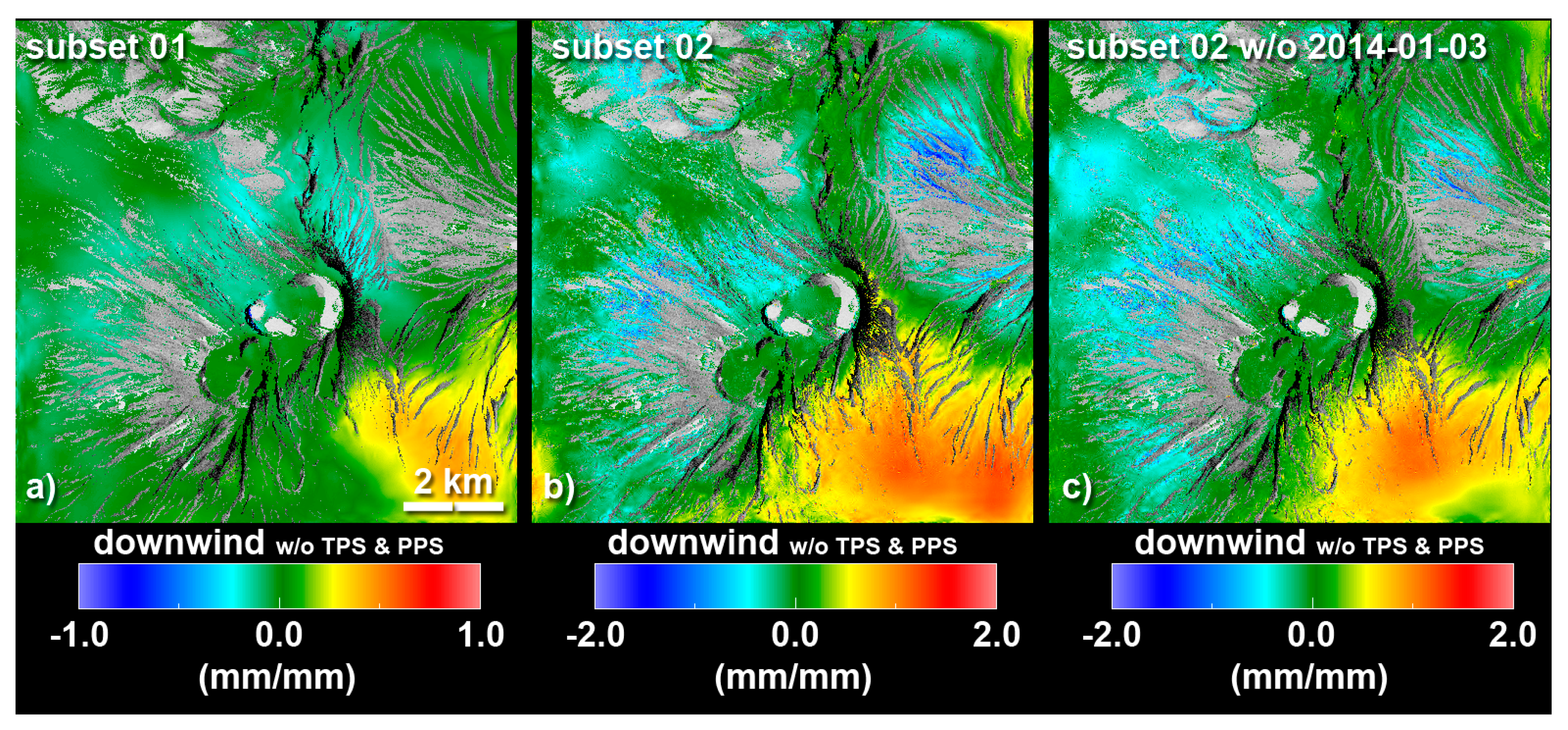
Appendix H. Gas Plume Related Phase Delays of DInSAR Time Series Subsets 01 and 02

Interferograms of DInSAR time series subsets 01 and 02 were decomposed, in order to separately examine the associated gas plume related phase delays. Estimates of gas plume related phase delays were computed for each of the two disjoint time series subsets, i.e., using a limited number of three (subset 01), and respectively four temporally interconnected interferograms (subset 02). Presented are the results obtained from the WBDD run, that was conducted omitting surface temperature and pressure priors, i.e., the phase delays associated to refractivity changes caused by atmospheric pressure and temperature variations were not prevented from leaking into the phase delay estimates obtained for the gas plume. Gas plume estimates of both subsets show a fan-shaped interferometric pattern indicating lengthening of the radar path over the south-eastern flank of Láscar volcano (depicted by yellow to orange colors in Figure A6a,b), which is in good agreement with the common direction of plume transport (see supplementary Figure A1c,d, Figure A2 and Figure A3 in Appendix D, where a detailed description of the wind field is given). Furthermore, this delay lengthening is coherent regarding the expected effect (Equation (1) in Smith and Weintraub, [66]), because the enhanced water vapor content of the volcanic gas plume is expected to increase the refractivity with respect to its surroundings. Negatively correlated phase delay patterns (depicted by cyan to blue colors in Figure A6a,b), which are distributed over the western flanks of Láscar and Aguas Calientes volcanoes, in contrast are incoherent in terms of the expected sign of the phase delay (Equation (1) in Smith and Weintraub, [66]) and thus cannot be attributed to the gas plume. They rather indicate the contribution of another process (or other processes), which was (were) not mitigated from the gas plume estimate. Subset 02 was additionally processed without the SAR acquisition of 3 January 2014, in order to display the resulting reduction of the phase delay amplitude in the repeating plume related signal (Figure A6c). PWV contents inside the plume and their respective differences were larger for SAR observations of subset 01, than they were for observations of subset 02 (Table 2), suggesting a stronger influence on the gas plume related phase delay signal of subset 01 (Figure A6a), if compared to subset 02 (Figure A6b,c). The amplitudes of the estimated phase delays displayed in Figure A6a–c are thus consistent with their respective input dSWD values (Table 3, column 4), and are also in accordance with humidity contrast between plume and atmosphere (Table 2).
Figure A6. Delay correlation maps depicting estimated interferometric gas plume patterns from (a) subset 01 and (b) subset 02. (c) Estimated interferometric pattern from subset 02, where the SAR observation of 03 Januray 2014 was omitted. All three estimates contain phase contributions of the temperature and pressure related phase screens (TPS & PPS not removed). Scales correspond to estimated delay (mm) per theoretical delay (mm). Upper and lower bounds of the scale bar are equal to unity in subset 01, but not in subset 02, indicating that the estimated delay in subset 02 was by a factor 2 larger than the theoretical delay.
Remotesensing 10 01514 g0a6

References

  1. Lengliné, O.; Marsan, D.; Got, J.L.; Pinel, V.; Ferrazzini, V.; Okubo, P.G. Seismicity and deformation induced by magma accumulation at three basaltic volcanoes. J. Geophys. Res. Solid Earth 2008, 113. [Google Scholar] [CrossRef] [Green Version]
  2. Morita, Y.; Nakao, S.; Hayashi, Y. A quantitative approach to the dike intrusion process inferred from a joint analysis of geodetic and seismological data for the 1998 earthquake swarm off the east coast of Izu Peninsula, central Japan. J. Geophys. Res. Solid Earth 2006, 111. [Google Scholar] [CrossRef] [Green Version]
  3. Watson, I.M.; Oppenheimer, C.; Voight, B.; Francis, P.W.; Clarke, A.; Stix, J.; Miller, A.; Pyle, D.M.; Burton, M.R.; Young, S.R.; et al. The relationship between degassing and ground deformation at Soufriere Hills Volcano, Montserrat. J. Volcanol. Geotherm. Res. 2000, 98, 117–126. [Google Scholar] [CrossRef]
  4. Kazahaya, R.; Aoki, Y.; Shinohara, H. Budget of shallow magma plumbing system at Asama Volcano, Japan, revealed by ground deformation and volcanic gas studies. J. Geophys. Res. Solid Earth 2015, 120, 2961–2973. [Google Scholar] [CrossRef] [Green Version]
  5. Girona, T.; Costa, F.; Newhall, C.; Taisne, B. On depressurization of volcanic magma reservoirs by passive degassing. J. Geophys. Res. Solid Earth 2014, 119, 8667–8687. [Google Scholar] [CrossRef] [Green Version]
  6. Tait, S.; Jaupart, C.; Vergniolle, S. Pressure, gas content and eruption periodicity of a shallow, crystallising magma chamber. Earth Planet. Sci. Lett. 1989, 92, 107–123. [Google Scholar] [CrossRef]
  7. Sparks, R.S.J. Dynamics of magma degassing. Geol. Soc. London Spec. Pub. 2003, 213, 5–22. [Google Scholar] [CrossRef]
  8. Green, D.N.; Neuberg, J. Waveform classification of volcanic low-frequency earthquake swarms and its implication at Soufrière Hills Volcano, Montserrat. J. Volcanol. Geotherm. Res. 2006, 153, 51–63. [Google Scholar] [CrossRef]
  9. Hooper, A.; Zebker, H.; Segall, P.; Kampes, B. A new method for measuring deformation on volcanoes and other natural terrains using InSAR persistent scatterers. Geophys. Res. Lett. 2004, 31, L23611. [Google Scholar] [CrossRef]
  10. Goldstein, R.M. Atmospheric Limitations to repeat-track radar interferometry. Geophys. Res. Lett. 1995, 22, 2517–2520. [Google Scholar] [CrossRef]
  11. Zebker, H.; Rosen, P.; Hensley, S. Atmospheric effects in interferometric synthetic aperture radar surface deformation and topographic maps. J. Geophys. Res. 1997, 102, 7547–7563. [Google Scholar] [CrossRef] [Green Version]
  12. Jung, J.; Kim, D.; Park, S.-E. Correction of Atmospheric Phase Screen in Time Series InSAR using WRF Model for Monitoring Volcanic Activities. IEEE Trans. Geosci. Remote Sens. 2014, 52, 2678–2689. [Google Scholar] [CrossRef]
  13. Foster, J.; Brooks, B.; Cherubini, T.; Shacat, C.; Businger, S.; Werner, C. Mitigating atmospheric noise for InSAR using a high resolution weather model. Geophys. Res. Lett. 2006, 33, L16304. [Google Scholar] [CrossRef]
  14. Pichelli, E.; Ferretti, R.; Cimini, D.; Perissin, D.; Montopoli, M.; Marzano, F.S.; Pierdicca, N. Water vapour distribution at urban scale using high-resolution numerical weather model and spaceborne SAR interferometric data. Nat. Hazard Earth Sys. Sci. 2010, 10, 121–132. [Google Scholar] [CrossRef] [Green Version]
  15. Ulmer, F.-G.; Adam, N. A Synergy Method to Improve Ensemble Weather Predictions and Differential SAR Interferograms. ISPRS J. Photogramm. Remote Sens. 2015, 109, 98–107. [Google Scholar] [CrossRef] [Green Version]
  16. Ulmer, F.-G.; Adam, N. Characterisation and improvement of the structure function estimation for application in PSI. ISPRS J. Photogramm. Remote Sens. 2017, 128, 40–46. [Google Scholar] [CrossRef]
  17. Bonforte, A.; Ferretti, A.; Prati, C.; Puglisi, G.; Rocca, F. Calibration of atmospheric effects on SAR interferograms by GPS and local atmosphere models: First results. J. Atmos. Sol. Terr. Phys. 2001, 63, 1343–1357. [Google Scholar] [CrossRef]
  18. Wadge, G.; Webley, P.W.; James, I.N.; Bingley, R.; Dodson, A.; Waugh, S.; Veneboer, T.; Puglisi, G.; Mattia, M.; Baker, D.; et al. Atmospheric models, GPS and InSAR measurements of the tropospheric water vapour field over Mount Etna. Geophys. Res. Lett. 2002, 29, 1905. [Google Scholar] [CrossRef]
  19. Rosen, P.A.; Henley, S.; Zebker, H.A.; Webb, F.H.; Fielding, E.J. Surface deformation and coherence measurements of Kilauea volcano, Hawaii, from SIR-C radar interferometry. J. Geophys. Res. 1996, 101, 23109–23125. [Google Scholar] [CrossRef]
  20. Wadge, G.; Mattioli, G.S.; Herd, R.A. Ground deformation at Soufrière Hills Volcano, Montserrat during 1998–2000 measured by radar interferometry and GPS. J. Volcanol. Geotherm. Res. 2006, 152, 157–173. [Google Scholar] [CrossRef]
  21. González, P.J.; Bagnardi, M.; Hooper, A.J.; Larsen, Y.; Marinkovic, P.; Samsonov, S.V.; Wright, T.J. The 2014–2015 eruption of Fogo volcano: Geodetic modeling of Sentinel-1 TOPS interferometry. Geophys. Res. Lett. 2015, 42, 9239–9246. [Google Scholar] [CrossRef]
  22. Wadge, G.; Costa, A.; Pascal, K.; Werner, C.; Webb, T. The variability of refractivity in the atmospheric boundary layer of a tropical island volcano measured by ground-based interferometric radar. Boundary-Layer Meteorol. 2016, 161, 309–333. [Google Scholar] [CrossRef]
  23. Saastamoinen, J. Introduction to practical computation of astronomical refraction. B. Géod. 1972, 106, 383–397. [Google Scholar] [CrossRef]
  24. Hanssen, R.F.; Weckwerth, T.M.; Zebker, H.A.; Klees, R. High-resolution water vapour mapping from interferometric radar measurements. Science 1999, 283, 1295–1297. [Google Scholar] [CrossRef]
  25. Mateus, P.; Nico, G.; Catalão, J. Can spaceborne SAR interferometry be used to study the temporal evolution of PWV? Atmos. Res. 2013, 119, 70–80. [Google Scholar] [CrossRef]
  26. Burton, M.R.; Oppenheimer, C.; Horrocks, L.; Francis, P.W. Remote sensing of CO2 and H2O emission rates from Masaya volcano, Nicaragua. Geology 2000, 28, 915–918. [Google Scholar] [CrossRef]
  27. Fiorani, L.; Colao, F.; Palucci, A.; Poreh, D.; Aiuppa, A.; Giudice, G. First-time lidar measurement of water vapor flux in a volcanic plume. Opt. Commun. 2011, 284, 1295–1298. [Google Scholar] [CrossRef] [Green Version]
  28. Bryan, S.; Clarke, A.; Vanderkluysen, L.; Groppi, C.; Paine, S.; Bliss, D.W.; Aberle, J.; Mauskopf, P. Measuring Water Vapor and Ash in Volcanic Eruptions With a Millimeter-Wave Radar/Imager. IEEE Trans. Geosci. Remote Sens. 2017, 55, 3177–3185. [Google Scholar] [CrossRef] [Green Version]
  29. Kern, C. The Difficulty of Measuring the Absorption of Scattered Sunlight by H2O and CO2 in Volcanic Plumes: A Comment on Pering et al. “A Novel and Inexpensive Method for Measuring Volcanic Plume Water Fluxes at High Temporal Resolution,” Remote Sensing 2017, 9, 146. Remote Sens. 2017, 9, 534. [Google Scholar] [CrossRef]
  30. Kern, C.; Masias, P.; Apaza, F.; Reath, K.A.; Platt, U. Remote measurement of high preeruptive water vapor emissions at Sabancaya volcano by passive differential optical absorption spectroscopy. J. Geophys. Res. Solid Earth 2017, 122, 3540–3564. [Google Scholar] [CrossRef]
  31. Gardeweg, M.C.; Sparks, R.S.J.; Matthews, S.J. Evolution of Lascar Volcano, northern Chile. J. Geol. Soc. 1998, 155, 89–104. [Google Scholar] [CrossRef]
  32. Matthews, S.J.; Sparks, R.S.J.; Gardeweg, M.C. The Piedras Grandes–Soncor eruptions, Lascar volcano, Chile; evolution of a zoned magma chamber in the central Andean upper crust. J. Petrol. 1999, 40, 1891–1919. [Google Scholar] [CrossRef]
  33. Tamburello, G.; Hansteen, T.H.; Bredemeyer, S.; Aiuppa, A.; Tassi, F. Gas emissions from five volcanoes in northern Chile, and implications for the volatiles budget of the Central Volcanic Zone. Geophys. Res. Lett. 2014, 41, 4961–4969. [Google Scholar] [CrossRef]
  34. Marín, J.C.; Pozo, D.; Mlawer, E.; Turner, D.D.; Curé, M. Dynamics of Local Circulations in Mountainous Terrain during the RHUBC-II Project. Mon. Weather Rev. 2013, 141, 3641–3656. [Google Scholar] [CrossRef]
  35. Giovanelli, R.; Darling, J.; Henderson, C.; Hoffman, W.; Barry, D.; Cordes, J.; Eikenberry, S.; Gull, G.; Keller, L.; Smith, J.D.; et al. The optical-infrared astronomical quality of high Atacama sites. II—Infrared characteristics. Publ. Astron. Soc. Pac. 2001, 113. [Google Scholar] [CrossRef]
  36. Matthews, S.J.; Jones, A.P.; Gardeweg, M.C. Lascar Volcano, northern Chile; evidence for steady-state disequilibrium. J. Petrol. 1994, 35, 401–432. [Google Scholar] [CrossRef]
  37. De Zeeuw-van Dalfsen, E.; Richter, N.; González, G.; Walter, T.R. Geomorphology and structural development of the nested summit crater of Láscar Volcano studied with Terrestrial Laser Scanner data and analogue modelling. J. Volcanol. Geotherm. Res. 2017, 329, 1–12. [Google Scholar] [CrossRef]
  38. Matthews, S.J.; Gardeweg, M.C.; Sparks, R.S.J. The 1984 to 1996 cyclic activity of Lascar Volcano, Northern Chile; cycles of dome growth, dome subsidence, degassing and explosive eruptions. Bull. Volcanol. 1997, 59, 72–82. [Google Scholar] [CrossRef]
  39. Pavez, A.; Remy, D.; Bonvalot, S.; Diament, M.; Gabalda, G.; Froger, J.L.; Julien, P.; Legrand, D.; Moisset, D. Insight into ground deformations at Lascar volcano (Chile) from SAR interferometry, photogrammetry and GPS data: Implications on volcano dynamics and future space monitoring. Remote Sens. Environ. 2006, 100, 307–320. [Google Scholar] [CrossRef]
  40. Richter, N.; Salzer, J.T.; de Zeeuw-van Dalfsen, E.; Perissin, D.; Walter, T.R. Constraints on the geomorphological evolution of the nested summit craters of Láscar Volcano from high spatio-temporal resolution TerraSAR-X interferometry. Bull. Volcanol. 2018, 80. [Google Scholar] [CrossRef]
  41. Tassi, F.; Aguilera, F.; Vaselli, O.; Medina, E.; Tedesco, D.; Huertas, A.D.; Poreda, R.; Kojima, S. The magmatic- and hydrothermal-dominated fumarolic system at the active crater of Lascar volcano, northern Chile. Bull. Volcanol. 2009, 71, 171–183. [Google Scholar] [CrossRef]
  42. Menard, G.; Moune, S.; Vlastélic, I.; Aguilera, F.; Valade, S.; Bontemps, M.; González, R. Gas and aerosol emissions from Lascar volcano (Northern Chile): Insights into the origin of gases and their links with the volcanic activity. J. Volcanol. Geotherm. Res. 2014, 287, 51–67. [Google Scholar] [CrossRef]
  43. González, C.; Inostroza, M.; Aguilera, F.; González, R.; Viramonte, J.; Menzies, A. Heat and mass flux measurements using Landsat images from the 2000-2004 period, Lascar volcano, northern Chile. J. Volcanol. Geotherm. Res. 2015, 301, 277–292. [Google Scholar] [CrossRef]
  44. Glaze, L.S.; Francis, P.W.; Rothery, D.A. Measuring thermal budgets of active volcanoes by satellite remote sensing. Nature 1989, 338, 144–146. [Google Scholar] [CrossRef]
  45. Oppenheimer, C.; Francis, P.W.; Rothery, D.A.; Carlton, R.W.; Glaze, L.S. Infrared image analysis of volcanic thermal features: Lascar Volcano, Chile, 1984–1992. J. Geophys. Res. Solid Earth 1993, 98, 4269–4286. [Google Scholar] [CrossRef]
  46. Wooster, M.J.; Rothery, D.A. Thermal monitoring of Lascar Volcano, Chile, using infrared data from the along-track scanning radiometer: A 1992–1995 time series. Bull. Volcanol. 1997, 58, 566–579. [Google Scholar] [CrossRef]
  47. Wooster, M.J. Long-term infrared surveillance of Lascar Volcano: Contrasting activity cycles and cooling pyroclastics. Geophys. Res. Lett. 2001, 28, 847–850. [Google Scholar] [CrossRef] [Green Version]
  48. Murphy, S.W.; Wright, R.; Oppenheimer, C.; Souza Filho, C.R. MODIS and ASTER synergy for characterizing thermal volcanic activity. Remote Sens. Environ. 2013, 131, 195–205. [Google Scholar] [CrossRef]
  49. Galle, B.; Johansson, M.; Rivera, C.; Zhang, Y.; Kihlman, M.; Kern, C.; Lehmann, T.; Platt, U.; Arellano, S.; Hidalgo, S. Network for Observation of Volcanic and Atmospheric Change (NOVAC)—A global network for volcanic gas monitoring: Network layout and instrument description. J. Geophys. Res. Atmos. 2010, 115. [Google Scholar] [CrossRef]
  50. Platt, U.; Stutz, J. Differential Optical Absorption Spectroscopy—Principles and Applications; Springer: Berlin/Heidelberg, Germany, 2008. [Google Scholar] [CrossRef]
  51. Vandaele, A.C.; Simon, P.C.; Guilmot, J.M.; Carleer, M.; Colin, R. SO2 absorption cross section measurement in the UV using a Fourier transform spectrometer. J. Geophys. Res. Atmos. 1994, 99, 25599–25605. [Google Scholar] [CrossRef]
  52. Voigt, S.; Orphal, J.; Bogumil, K.; Burrows, J.P. The temperature dependence (203–293K) of the absorption cross sections of O3 in the 230–850 nm region measured by Fourier-transform spectroscopy. J. Photoch. Photobiol. A Chem. 2001, 143, 1–9. [Google Scholar] [CrossRef]
  53. Solomon, S.; Schmeltekopf, A.L.; Sanders, R.W. On the interpretation of zenith sky absorption measurements. J. Geophys. Res. Atmos. 1987, 92, 8311–8319. [Google Scholar] [CrossRef]
  54. Kurucz, R.L.; Furenlid, I.; Brault, J.; Testerman, L. Solar Flux Atlas from 296 to 1300 nm; National Solar Observatory: Sunspot, NM, USA, 1984; 240p. [Google Scholar]
  55. Aiuppa, A.; Moretti, R.; Federico, C.; Giudice, G.; Gurrieri, S.; Liuzzo, M.; Papale, P.; Shinohara, H.; Valenza, M. Forecasting Etna eruptions by real-time observation of volcanic gas composition. Geology 2007, 35, 1115–1118. [Google Scholar] [CrossRef]
  56. Shinohara, H.; Aiuppa, A.; Guidice, G.; Gurrieri, S.; Liuzzo, M. Variation of H2O/CO2 and CO2/SO2 ratios of volcanic gases discharged by continuous degassing of Mount Etna volcano, Italy. J. Geophys. Res. Solid Earth 2008, 113, B09203. [Google Scholar] [CrossRef]
  57. Aiuppa, A.; Bertagnini, A.; Métrich, N.; Moretti, R.; Di Muro, A.; Liuzzo, M.; Tamburello, G. A model of degassing for Stromboli volcano. Earth Planet. Sci. Lett. 2010, 295, 195–204. [Google Scholar] [CrossRef] [Green Version]
  58. Matsushima, N.; Shinohara, H. Visible and invisible volcanic plumes. Geophys. Res. Lett. 2006, 33, L24309. [Google Scholar] [CrossRef]
  59. Ebmeier, S.K.; Sayer, A.M.; Grainger, R.G.; Mather, T.A.; Carboni, E. Systematic satellite observations of the impact of aerosols from passive volcanic degassing on local cloud properties. Atmos. Chem. Phys. 2014, 14, 10601–10618. [Google Scholar] [CrossRef]
  60. Eineder, M.; Adam, N. A flexible system for the generation of interferometric SAR products. In Proceedings of the International Geoscience and Remote Sensing Symposium IGARSS’97. Remote Sensing—A Scientific Vision for Sustainable Development, Singapore, 3–8 August 1997. [Google Scholar] [CrossRef]
  61. Bevis, M.; Businger, S.; Herring, T.A.; Rocken, C.; Anthes, R.A.; Ware, R.H. GPS meteorology: Remote sensing of atmospheric water vapour using the Global Positioning System. J. Geophys. Res. Atmos. 1992, 97, 15787–15801. [Google Scholar] [CrossRef]
  62. Ulmer, F.-G. On the accuracy gain of electromagnetic wave delay predictions derived by the digital filter initialization technique. J. Appl. Remote Sens. 2016, 10, 016007:1–016007:7. [Google Scholar] [CrossRef]
  63. Ulmer, F.-G. Cinderella: Method Generalisation of the Elimination Process to Filter Repeating Patterns. In Proceedings of the 2015 IEEE International Conference on Digital Signal Processing (DSP), Singapore, 21–24 July 2015. [Google Scholar] [CrossRef]
  64. Selesnick, I.W.; Baraniuk, R.G.; Kingsbury, N.C. The dual-tree complex wavelet transform. IEEE Signal Process. Mag. 2005, 22, 123–151. [Google Scholar] [CrossRef] [Green Version]
  65. Fattahi, H.; Amelung, F. DEM error correction in InSAR time series. IEEE Trans. Geosci. Remote Sens. 2013, 51, 4249–4259. [Google Scholar] [CrossRef]
  66. Smith, E.K.; Weintraub, S. The Constants in the Equation for Atmospheric Refractive Index at Radio Frequencies. Proc. IRE 1953, 41, 1035–1037. [Google Scholar] [CrossRef] [Green Version]
  67. Oppenheimer, C.; Fischer, T.P.; Scaillet, B. Volcanic degassing: Process and impact. In Treatise on Geochemistry, 2nd ed.; Elsevier Ltd.: Amsterdam, The Netherlands, 2014; Volume 4, pp. 111–179. [Google Scholar] [CrossRef]
  68. Battaglia, M.; Troise, C.; Obrizzo, F.; Pingue, F.; De Natale, G. Evidence for fluid migration as the source of deformation at Campi Flegrei caldera (Italy). Geophys. Res. Lett. 2006, 33. [Google Scholar] [CrossRef] [Green Version]
  69. Samsonov, S.V.; Tiampo, K.F.; Camacho, A.G.; Fernández, J.; González, P.J. Spatiotemporal analysis and interpretation of 1993–2013 ground deformation at Campi Flegrei, Italy, observed by advanced DInSAR. Geophys. Res. Lett. 2014, 41, 6101–6108. [Google Scholar] [CrossRef]
  70. Ruch, J.; Manconi, A.; Zeni, G.; Solaro, G.; Pepe, A.; Shirzaei, M.; Walter, T.R.; Lanari, R. Stress transfer in the Lazufre volcanic area, central Andes. Geophys. Res. Lett. 2009, 36. [Google Scholar] [CrossRef] [Green Version]
  71. Werner, C.; Hurst, T.; Scott, B.; Sherburn, S.; Christenson, B.W.; Britten, K.; Cole-Barker, J.; Mullan, B. Variability of passive gas emissions, seismicity, and deformation during crater lake growth at White Island Volcano, New Zealand, 2002–2006. J. Geophys. Res. Solid Earth 2008, 113. [Google Scholar] [CrossRef] [Green Version]
  72. Chiodini, G.; Caliro, S.; De Martino, P.; Avino, R.; Gherardi, F. Early signals of new volcanic unrest at Campi Flegrei caldera? Insights from geochemical data and physical simulations. Geology 2012, 40, 943–946. [Google Scholar] [CrossRef]
  73. Dinger, F.; Bobrowski, N.; Warnach, S.; Bredemeyer, S.; Hidalgo, S.; Arellano, S.; Galle, B.; Platt, U.; Wagner, T. Periodicity in the BrO/SO2 molar ratios in the volcanic gas plume of Cotopaxi and its correlation with the Earth tides during the eruption in 2015. Solid Earth Discuss. 2018, 1–28. [Google Scholar] [CrossRef]
  74. Fujiwara, S.; Rosen, P.A.; Tobita, M.; Murakami, M. Crustal deformation measurements using repeat-pass JERS 1 synthetic aperture radar interferometry near the Izu Peninsula, Japan. J. Geophys. Res. Solid Earth 1998, 103, 2411–2426. [Google Scholar] [CrossRef] [Green Version]
  75. Knospe, S.; Jonsson, S. Covariance estimation for dInSAR surface deformation measurements in the presence of anisotropic atmospheric noise. IEEE Trans. Geosci. Remote Sens. 2010, 48, 2057–2065. [Google Scholar] [CrossRef]
  76. Aumento, F. Radon tides on an active volcanic island: Terceira, Azores. Geofís. Int. 2002, 41, 499–505. [Google Scholar]
  77. Bredemeyer, S.; Hansteen, T.H. Synchronous degassing patterns of the neighbouring volcanoes Llaima and Villarrica in south-central Chile: The influence of tidal forces. Int. J. Earth Sci. 2014, 103, 1999–2012. [Google Scholar] [CrossRef] [Green Version]
  78. Zimmer, M.; Walter, T.R.; Kujawa, C.; Gaete, A.; Franco-Marin, L. Thermal and gas dynamic investigations at Lastarria volcano, Northern Chile. The influence of precipitation and atmospheric pressure on the fumarole temperature and the gas velocity. J. Volcanol. Geotherm. Res. 2017, 346, 134–140. [Google Scholar] [CrossRef]
  79. NOAA Air Resources Laboratory: READY Archived Meteorology. Available online: https://ready.arl.noaa.gov/READYamet.php (accessed on 18 September 2018).
  80. Edmonds, M.; Herd, R.A.; Galle, B.; Oppenheimer, C.M. Automated, high time-resolution measurements of SO2 flux at Soufrière Hills Volcano, Montserrat. Bull. Volcanol. 2003, 65, 578–586. [Google Scholar] [CrossRef]
  81. Global Volcanism Program. Report on Lascar (Chile). In Bulletin of the Global Volcanism Network; Venzke, E., Ed.; Smithsonian Institution: Washington, DC, USA, 2015; Available online: https://volcano.si.edu/showreport.cfm?doi=10.5479/si.GVP.BGVN201506-355100 (accessed on 18 September 2018).
  82. Giovanelli, R. Optical seeing and infrared atmospheric transparency in the upper Atacama desert. Astronomical Site Evaluation in the Visible and Radio Range. In Astronomical Site Evaluation in the Visible and Radio Range. ASP Conference Proceedings, 266; Vernin, J., Benkhaldoun, Z., Muñoz-Tuñón, C., Eds.; Astronomical Society of the Pacific: San Francisco, CA, USA, 2002; p. 366. ISBN 1-58381-106-0. [Google Scholar]
  83. Vuille, M. Atmospheric circulation over the Bolivian Altiplano during dry and wet periods and extreme phases of the Southern Oscillation. Int. J. Climatol. 1999, 19, 1579–1600. [Google Scholar] [CrossRef] [Green Version]
  84. Messerli, B.; Grosjean, M.; Bonani, G.; Bürgi, A.; Geyh, M.A.; Graf, K.; Ramseyer, K.; Romero, H.; Schotterer, U.; Schreier, H.; Vuille, M. Climate change and natural resource dynamics of the Atacama Altiplano during the last 18,000 years: A preliminary synthesis. Mt. Res. Dev. 1993, 117–127. [Google Scholar] [CrossRef]
  85. Vuille, M.; Ammann, C. Regional snowfall patterns in the high, arid Andes. Clim. Chang. 1997, 36, 413–423. [Google Scholar] [CrossRef]
  86. Mori, T.; Mori, T.; Kazahaya, K.; Ohwada, M.; Hirabayashi, J.I.; Yoshikawa, S. Effect of UV scattering on SO2 emission rate measurements. Geophys. Res. Lett. 2006, 33. [Google Scholar] [CrossRef]
  87. Symonds, R.B.; Gerlach, T.M.; Reed, M.H. Magmatic gas scrubbing: Implications for volcano monitoring. J. Volcanol. Geotherm. Res. 2001, 108, 303–341. [Google Scholar] [CrossRef]
  88. Rodríguez, L.A.; Watson, I.M.; Edmonds, M.; Ryan, G.; Hards, V.; Oppenheimer, C.M.; Bluth, G.J. SO2 loss rates in the plume emitted by Soufrière Hills volcano, Montserrat. J. Volcanol. Geotherm. Res. 2008, 173, 135–147. [Google Scholar] [CrossRef] [Green Version]
  89. Beirle, S.; Hörmann, C.; Penning de Vries, M.; Dörner, S.; Kern, C.; Wagner, T. Estimating the volcanic emission rate and atmospheric lifetime of SO2 from space: A case study for Kīlauea volcano, Hawaii. Atmos. Chem. Phys. 2014, 14, 8309–8322. [Google Scholar] [CrossRef]
  90. Samsonov, S.V.; Trishchenko, A.P.; Tiampo, K.; González, P.J.; Zhang, Y.; Fernández, J. Removal of systematic seasonal atmospheric signal from interferometric synthetic aperture radar ground deformation time series. Geophys. Res. Lett. 2014, 41, 6123–6130. [Google Scholar] [CrossRef] [Green Version]
  91. Johansson, M.E.B. Application of passive DOAS for studies of megacity air pollution and volcanic gas emissions. Ph.D. Thesis, Chalmers University of Technology, Gothenburg, Sweden, 2009. [Google Scholar]
  92. Marquard, L.C.; Wagner, T.; Platt, U. Improved air mass factor concepts for scattered radiation differential optical absorption spectroscopy of atmospheric species. J. Geophys. Res. Atmos. 2000, 105, 1315–1327. [Google Scholar] [CrossRef] [Green Version]
  93. McClatchey, R.A.; Fenn, R.W.; Selby, J.A.; Volz, F.E.; Garing, J.S. Optical properties of the atmosphere (No. AFCRL-72-0497); Air Force Cambridge Research Laboratories, Hanscom AFB: Bedford, MA, USA, 1972. [Google Scholar]
  94. Wagner, T.; Beirle, S.; Grzegorski, M.; Platt, U. Global trends (1996–2003) of total column precipitable water observed by Global Ozone Monitoring Experiment (GOME) on ERS-2 and their relation to near-surface temperature. J. Geophys. Res. Atmos. 2006, 111, D12102. [Google Scholar] [CrossRef]
  95. Granger, R.J. An examination of the concept of potential evaporation. J. Hydrol. 1989, 111, 9–19. [Google Scholar] [CrossRef]
  96. Horrocks, L.A.; Oppenheimer, C.; Burton, M.R.; Duffell, H.J. Compositional variation in tropospheric volcanic gas plumes: Evidence from ground-based remote sensing. Geol. Soc. Lond. Spec. Pub. 2003, 213, 349–369. [Google Scholar] [CrossRef]
  97. Singh, V.P.; Xu, C.Y. Evaluation and generalization of 13 mass-transfer equations for determining free water evaporation. Hydrol. Process. 1997, 11, 311–323. [Google Scholar] [CrossRef]
  98. Dalton, J. Experimental essays on the constitution of mixed gases on the force of steam or vapor from water and other liquids in different temperatures, both in a Torricellian vacuum and in air; on evaporation and on the expansion of gases by heat. Mem. Lit. Philos. Soc. Manch. 1802, 5, 535–602. [Google Scholar]
  99. Penman, H.L. Natural evaporation from open water, bare soil, and grass. P. Roy. Soc. Lond. 1948, A193, 120–146. [Google Scholar] [CrossRef]
  100. Van Bavel, C.H.M. Potential evaporation: The combination concept and its experimental verification. Water Resour. Res. 1996, 2, 455–467. [Google Scholar] [CrossRef]
  101. Tennekes, H. The logarithmic wind profile. J. Atmos. Sci. 1973, 30, 234–238. [Google Scholar] [CrossRef]
  102. Mason, P.J. The formation of areally-averaged roughness lengths. Q. J. Roy. Meteorol. Soc. 1988, 114, 399–420. [Google Scholar] [CrossRef]
  103. Magnus, G. Versuche über die Spannkräfte des Wasserdampfs. Ann. Phys. 1844, 137, 225–247. [Google Scholar] [CrossRef]
  104. Sonntag, D. Important new values of the physical constants of 1986, vapor pressure formulations based on the ITS-90, and psychrometer formulae. Z. Meteorol. 1990, 70, 340–344. [Google Scholar]
  105. Alduchov, O.A.; Eskridge, R.E. Improved Magnus form approximation of saturation vapor pressure. J. Appl. Meteorol. 1996, 35, 601–609. [Google Scholar] [CrossRef]
  106. Jones, F.E.; Harris, G.L. ITS-90 density of water formulation for volumetric standards calibration. J. Res. Natl. Inst. Stand. 1992, 97, 335–340. [Google Scholar] [CrossRef] [PubMed]
  107. Plate, E.J.; Quraishi, A.A. Modeling of Velocity Distributions Inside and Above Tall Crops. J. Appl. Meteorol. 1965, 4, 400–408. [Google Scholar] [CrossRef] [Green Version]
  108. Hansen, F.V. Surface Roughness Lengths (No. ARL-TR-61); Army Research Lab White Sands Missile Range NM: Adelphi, MD, USA, 1993; pp. 88002–85501. [Google Scholar]
  109. Garrison, J.D.; Adler, G.P. Estimation of precipitable water over the United States for application to the division of solar radiation into its direct and diffuse components. Sol. Energy 1990, 44, 225–241. [Google Scholar] [CrossRef]
  110. Nann, S.; Riordan, C. Solar spectral irradiance under clear and cloudy skies: Measurements and a semiempirical model. J. Appl. Meteorol. 1991, 30, 447–462. [Google Scholar] [CrossRef]
Figure 1. Láscar and adjacent Aguas Calientes volcanoes. The location of the scanning Mini-DOAS station is indicated by the white dot on the southern flank of Aguas Calientes volcano. (a) Aster visible range composite of 29 April 2013 draped onto SRTM-1 grid; (b) Close-up of high temperature fumaroles in the active crater; (c) View from the southern crater rim towards NNW into the active crater of Láscar showing fumarolic activity during the Multi-GAS survey on the Southern crater rim on 2 December 2012. The white bounding box framing the area shown in (b) roughly spans 200 m in width and 100 m in height; (d) Panoramic view from South towards NNW showing a dispersed gas plume emanating from Láscars’ active crater on 5 December 2012, and drifting towards SE, which corresponds to the main transport direction during daylight time. Distance between Mini-DOAS in the foreground and active crater in the background of the image is about 6 km.
Remotesensing 10 01514 g001
Figure 2. Spatio-temporal relationships between the methods used for the gas plume estimate. (a) Sketch showing the measurement geometry and location of the Multi-GAS and scanning Mini-DOAS instruments at Láscar volcano during an overpass of TerraSAR-X. Refractive delay of the radar occurs inside the volcanic plume, which is heading towards East, due to predominantly westerly winds. See text for discussion; (b) Date versus time plot depicting acquisition times of scanning DOAS measurements and SAR images. Measurement times are indicated using Coordinated Universal Time (UTC), which is offset by +3 h with respect to Chile Summer Time (CLST). Red arrows indicate the temporal offset between SAR images and scanning DOAS data chosen for analysis; (c) Spatial and temporal baselines of SAR images used in DInSAR time series subsets 01 (blue) and 02 (red). Master scenes of subset 01 and subset 02 are from 18 October 2013 and 12 December 2013, respectively, and each computed interferogram is represented by a line between the corresponding two images.
Remotesensing 10 01514 g002
Figure 3. Technical diagram depicting the processing steps of the WBDD algorithm. In a DInSAR time series each DInSAR pixel (respectively range azimuth position) is characterized by a certain temporal evolution of its differential signal strength. Computation of the D T - W T representations of each DInSAR enables to capture the temporal evolution of the signal strength of all SAR pixels of the DInSAR time series by means of a small number of complex wavelet coefficients. Similarly each process which causes changes in SAR signal strength can be described by a time series, which reflects the temporal variations of the process (e.g., variations of water vapor contents in the volcanic gas plume, variations in spatial baseline, relative humidity, ground temperature, and pressure). The algorithm uses the time series of these processes as an a priori knowledge of a related possible change in SAR signal strength and assigns the SAR signals to their likely causes by comparison of the prior time series with the temporal evolution of SAR signal strength at each range azimuth position, which decomposes the interferograms into different phase screens.
Remotesensing 10 01514 g003
Figure 4. (a) Time series of PWV contents determined for plume cross-sections recorded by scanning DOAS on days with TerraSAR-X acquisitions (18 December 2013 to 16 February 2014). The time scale is not linear. Result without consideration of evaporation; (b) Daily average PWV contents in the centerline of the plume (stippled line) and the bulk plume (solid line), which are representative for the moisture distribution above the crater rim on days with available SAR acquisitions; (c) Time series of potential evaporation rates at plume height above the summit of Láscar volcano. Evaporation rates at the times of SAR observations are indicated by red (master scenes) and blue (slave scenes) dots; (d) Time series of wind speeds at summit altitude used for calculation of potential evaporation rates; (e) Time series of PWV contents in plume cross-sections considering downwind evaporation; (f) Daily average PWV content in the centerline of the plume (stippled line) and the bulk plume (solid line) downwind of the volcano on days with available SAR acquisitions.
Remotesensing 10 01514 g004
Figure 5. (a) PWV contents in plume cross-sections obtained for the downwind portion of the volcanic gas plume on acquisition dates of SAR master and slave scenes, and (be) corresponding DInSAR maps (10 × 10 km in azimuth and range direction). Scales of the DInSAR maps indicate range change in units of mm, and are unique to each image using the same scale bounds for the sake of comparability with other phase contributions. Incoherent areas are masked out; (b) Coarsely corrected DInSAR maps used for decomposition analysis and retrieval of the gas plume estimate. DEM and major APS contributions derived from WRF were removed; (c) Phase difference maps of the gas plume estimates obtained for the downwind portion of the volcanic gas plume. Corresponding theoretical dSWDs are indicated in the upper right corner of each map; (d) DInSAR maps from 5b, where the phase contributions of the gas plume were removed; (e) Linear deformation estimates obtained from the refined correction using the delay estimates obtained from WBDD analysis.
Remotesensing 10 01514 g005
Figure 6. (ah) Delay correlation maps depicting the estimated repeating patterns of SAR delays obtained from priors included in the WBDD analysis. Location of active crater is indicated by the red circle; (a) Delay estimate for the gas plume aloft the crater (bd) Delay estimates for the downwind portion of the gas plume (b) with and (c) without additional removal of pressure and temperature dependent phase screens by including/excluding respective priors in the WBDD analysis; (d) Gas plume estimate as in c), however omitting the SAR observation of 3 January 2014. Scales correspond to estimated delay (mm) per theoretical delay (mm). Scale bar limits of the gas plume estimate obtained for the proximal part of the plume above the crater indicate that theoretical delays are by a factor 100 smaller than the delay estimate. Upper and lower limits of the scale bars of the estimates obtained for the downwind portion of the gas plume are equal to unity, indicating concurrence of theoretical and estimated delay. The red to yellow colored signature in the lower right corner of the image indicates a lengthening of the delay, where the effect of H2O emissions is large. The affected area corresponds to the most common plume transport directions (see Appendix D, Figure A3a,b) and locations where the volcanic plume regularly touches the ground (fumigation); (e) Estimates of surface temperature and (f) surface pressure related delays. Scales indicate mm estimated delay per Kelvin, respectively hPa of the input prior; (g) Delay estimate obtained for the relative humidity prior (h) Delay estimate for the spatial baseline prior; (i) Scatter plot of theoretical delay (mm) versus determined signal strength of the gas plume contribution in the DInSARs used for the gas plume estimate in (b). Each asterisk symbol represents one of the DInSARs and corresponding slave dates (mm-dd) are indicated.
Remotesensing 10 01514 g006
Figure 7. (a) H2O emission rates from Láscar volcano along with a sequence of Aster, Landsat-8 and EO-1 ALI scenes depicting snow and cloud coverage (upper row: false-color composites of SWIR, NIR and visible red spectral bands; lower row: true-color images using a combination of visible red, green and blue spectral bands). Days with incandescence observations are indicated by stippled grey vertical lines. Precipitation events that were recorded in Toconao (on 10 November 2013, 17 January 2014, and 26 January 2014) are indicated by vertical blue lines, including information on amount and duration of the events; (b) Background atmospheric PWV contents estimated from GDAS1 soundings above Láscar volcano (red curve), compared to radiometer measurements conducted at APEX (blue curve). Good agreement between the two curves reflects similar weather conditions caused by a similar morphologic exposition of both sites, and may additionally be attributed to the coarse spatial resolution of the GDAS1 data. PWV estimates for the times of SAR observations are indicated by red (master scene) and blue (slave scene) dots, respectively.
Remotesensing 10 01514 g007
Table 1. Combinations of SAR acquisitions used in DInSAR time series subsets 01 & 02, and their respective spatial and temporal baselines.
Master Scene Date (yyyy-mm-dd)Slave Scene Date (yyyy-mm-dd)Spatial Baseline (m)Temporal Baseline (Days)
Subset 01
2013-12-122013-11-2011.8−22
2013-12-122013-12-016.211
2013-12-122014-02-05−0.555
Subset 02
2013-10-182013-12-2316.666
2013-10-182014-01-03−23.577
2013-10-182014-01-14688
2013-10-182014-02-16−1.3121
Table 2. Combinations of SAR acquisitions used in DInSAR time series subsets 01 and 02, and corresponding estimates of PWV contents inside the plume, and the ambient atmosphere are listed along with conversion factors Π T S 1 used for calculation of theoretical SWDs.
SceneDate (yyyy-mm-dd)PWV (mm) Π T S 1   ( mm ) SWD (mm)
Crater Rim Plume CenterDownwind Plume CenterDownwind Bulk PlumeAverage Background AtmosphereCrater rim Plume CenterDownwind Plume CenterDownwind Bulk PlumeAverage Background Atmosphere
Subset 01
Master2013-12-120.0124.31.32.16.420.09634.5910.3817.25
Slave2013-11-200.0119.42.41.06.580.08977.0120.168.46
Slave2013-12-010.0094.31.10.76.390.07234.448.615.97
Slave2014-02-050.0100.80.24.36.410.0846.431.7634.85
totals 0.04218.85.08.3 0.341152.4640.9166.52
Subset 02
Master2013-10-180.0072.20.70.76.510.05917.985.515.31
Slave2013-12-230.0091.10.35.26.430.0758.912.1041.48
Slave2014-01-030.0131.80.53.06.380.10114.153.6423.96
Slave2014-01-140.0110.90.23.66.390.0917.271.6729.06
Slave2014-02-160.0154.91.11.76.440.12139.309.1113.78
totals 0.05610.92.714.1 0.44787.6022.03113.58
Table 3. Priors used in the WBDD analysis include two gas plume related differential slant wet delay (dSWD) time series for the proximal and distal portions of the plume, differential time series of relative humidity, surface temperature and surface pressure, as well as spatial and temporal baselines. Dirac-function priors for the single event APS estimation are not displayed.
Master Scene Date (yyyy-mm-dd)Slave Scene Date (yyyy-mm-dd)Gas plume Related Priors (dSWD)Troposphere Related PriorsTopography Related Priors
Crater Rim Plume Center (mm)Downwind Bulk Plume (mm)Relative Humidity (%)Surface Temperature (K)Surface Pressure (hPa)Spatial Baseline (m)Temporal Baseline (Days)
Subset 01
2013-12-122013-11-200.007−9.78−0.054.600.9611.8−22
2013-12-122013-12-010.0241.7718.09−3.32−1.496.2−11
2013-12-122014-02-050.0138.62−37.950.050.02−0.555
Subset 02
2013-10-182013-12-23−0.0163.40−48.55−4.57−0.1916.666
2013-10-182014-01-03−0.0421.87−17.55−3.051.85−23.577
2013-10-182014-01-14−0.0323.84−29.09−4.35−1.09688
2013-10-182014-02-16−0.062−3.60−9.42−2.73−0.45−1.3121

