Evaluating Intra-Field Spatial Variability for Nutrient Management Zone Delineation through Geospatial Techniques and Multivariate Analysis

Abstract

This research study underscores the importance of effectively managing soil nutrients in a site-specific manner to enhance crop productivity while considering the spatial variability of the soil. The objective is to identify subfields with similar soil characteristics, referred to as management zones (MZs), to promote sustainable land utilization. This study was conducted in two central pivot fields located in Southern Idaho, USA, where barley and sugar beets were grown. Soil samples were collected from each field in a grid pattern and analyzed for various chemical properties. These properties included soil pH, organic matter, cation exchange capacity, excess lime, electrical conductivity, total inorganic nitrogen, phosphorus, potassium, calcium, magnesium, zinc, iron, manganese, copper, and boron. Descriptive statistics and normality assessments were performed, and the coefficient of variation was calculated to assess the heterogeneity of soil properties, revealing significant variability. To determine the spatial variability of soil properties, ordinary kriging was used revealing diverse spatial patterns for each location and soil variable examined with moderate to strong spatial dependence. To develop the MZs, a combination of principal component analysis and fuzzy k-means clustering was utilized, and specific parameters that represented the overall variability of soil properties in each field were identified. Based on the identified parameters, two clusters were created in each field. The first management zone (MZ1) exhibited lower values of soil pH, excess lime content, and electrical conductivity compared to the MZ2. Consequently, higher crop productivity was observed in MZ1 in both fields. The biomass yields of barley and sugar beets in MZ1 surpassed those in MZ2. This study highlights the effectiveness of the methodology employed to delineate MZs, which can be instrumental in precise soil nutrient management and maximizing crop productivity.

1. Introduction

Soil plays a crucial role as the foundation for crop cultivation, but its properties are constantly changing [1]. In scenarios where monoculture practices are employed and climatic conditions remain uniform, soil properties become the primary determinants affecting crop production. Consequently, variations in crop properties are primarily attributable to the heterogeneity of soil properties. Furthermore, even minor disparities in soil attributes can trigger spatially variable crop yields within a uniformly managed crop stand [2]. The large-scale variation in soil properties within a field is influenced by factors such as climatic conditions, topographical relief, parent material, and soil management practices [1,3]. By being aware of the spatial heterogeneity of soil chemical properties within a field, farmers can implement more effective management strategies for sustainable agricultural production [4].

Precision agriculture technologies have the potential to significantly increase crop yield while minimizing the negative environmental impact caused by excessive agrochemical use [5]. One key strategy in precision agriculture is through the use of variable-rate input applications [6]. The core principle of precision agriculture lies in utilizing extensive soil and crop data to develop site-specific management approaches, as emphasized by [7]. These approaches consider the variations in soil and crop yield within a field and establish homogeneous MZs, as described by [8]. Management zones are essentially uniform regions defined by spatially variable attributes [9]. These subdivisions are derived from similarities in crop yield and soil attributes, enabling tailored agricultural input requirements for each subregion. For instance, fertilizer application can be customized based on the specific needs of each management zone [10,11], potentially reducing the amount of fertilizer applied to the field. Well-established MZs not only facilitate variable-rate applications but also provide crucial support for the comprehensive 4R Nutrient Stewardship program. This program addresses the four key aspects of nutrient management: source, rate, timing, and placement, all within the specific context of a cropping system [12].

Numerous researchers have utilized geostatistics to investigate the spatial variability and distribution of soil properties across different scales [13,14,15,16,17]. These studies have focused on establishing soil MZs in diverse agroecosystems to facilitate site-specific soil management. Additional research has also sought to use information on soil spatial variability to establish common subregions of soil for targeted agronomic interventions and management. Various approaches have been employed to define these MZs. For instance, some researchers have integrated farmer expertise with visual landscape differences derived from aerial photography [18], while others incorporated yield information to designate productivity zones [19]. Multivariate approaches such as cluster analysis have been used to define MZs using a suite of soil variables including soil fertility [20]. Additionally, apparent soil electrical conductivity has been utilized to define MZs [21].

Principal component analysis serves as a multivariate analysis technique that simplifies the description of a set of interconnected variables by summarizing and aggregating the sources of spatial variability. It identifies the minimum data set (MDS) and generates new orthogonal variables known as principal components (PCs) [22,23]. PCA is widely employed as a data reduction method to derive smaller groups from multivariate data, consistently producing optimal outcomes in recent research endeavors focused on delineating MZs [22,24,25,26].

One approach is to group measured soil data using PCA to explain the variations in grain and biomass yields [27]. Furthermore, recent studies [22,28,29,30] have demarcated MZs through integrated approaches, amalgamating geostatistics, PCA, and fuzzy k-means clustering algorithms, all using soil fertility data. However, most of these investigations have primarily concentrated on soil macronutrients, such as nitrogen (N), phosphorus (P), and potassium (K) [31,32], along with soil pH [33]. Meanwhile, there has been a significant lack of research that comprehensively considers both macro and micronutrients, as well as other critical soil parameters, including calcium (Ca), magnesium (Mg), manganese (Mn), zinc (Zn), iron (Fe), copper (Cu), boron (B), cation exchange capacity (CEC), EC, and excess lime [34].

The agricultural sector plays a significant role in contributing to the gross domestic product and holds the potential for enhanced profitability in states like Idaho, which is the top producer of barley and potatoes, the second-largest producer of sugar beets and hops, and the third-largest producer of hay [35]. The primary production areas for these commodities are concentrated in Southern Idaho. Agricultural producers in this region, akin to counterparts elsewhere, face the challenge of efficiently managing irrigation water and optimizing soil fertility across extensive and spatially heterogeneous fields.

The prolific agricultural sector in Southern Idaho can be attributed to favorable climatic conditions and the promising economic prospects it offers. However, the extensive application of mineral fertilizers is a common practice due to the prevalent issues of low soil fertility and suboptimal fertilizer usage recommendations, primarily aimed at enhancing crop yields. For example, deficiencies in soil nitrogen levels have been observed to have adverse effects on sugar beet root yield. Conversely, an excessive presence of nitrogen in the soil has been linked to reduced sucrose content and decreased sucrose recovery due to heightened nitrate impurities, both indicators of low beet end-use quality [36]. While N management is generally more controllable, maintaining appropriate levels of essential soil nutrients, such as P, K, and micronutrients, is equally crucial to attaining optimal sugar yields. Unfortunately, it is a common misconception among growers in Southern Idaho that a robust sugar beet canopy is directly correlated with high yields, which may lead to excessive N application in an attempt to maximize sugar production amounts [36,37]. Hence, the identification of nutrient-related constraints and the implementation of effective management strategies are important to maintain or enhance crop productivity [38].

Currently, nutrient management practices for large irrigated fields in Southern Idaho rely on standardized and uniform recommendations applied across large regions. However, this approach often results in the over-application of nutrients in areas with high nutrient levels and insufficient nutrient application in regions with low nutrient concentrations [37]. The existing knowledge regarding the spatial heterogeneity of soil properties and the delineation of soil MZs for crop cultivation expansion in Southern Idaho is limited. Given these considerations, it is imperative to address the spatial variability of crucial soil chemical attributes. This is essential for the development of site-specific soil management strategies and the formulation of well-informed crop management decisions. Acknowledging the pivotal role of soil spatial variability in the identification of nutrient management zones, this research was undertaken with the following objectives: (i) to characterize the spatial variability of soil chemical attributes that significantly impact crop productivity in Southern Idaho agriculture fields, and (ii) to delineate nutrient management zones in crop fields through the integration of geostatistical analysis and principal component analysis applied to select soil chemical attributes.

2. Materials and Methods

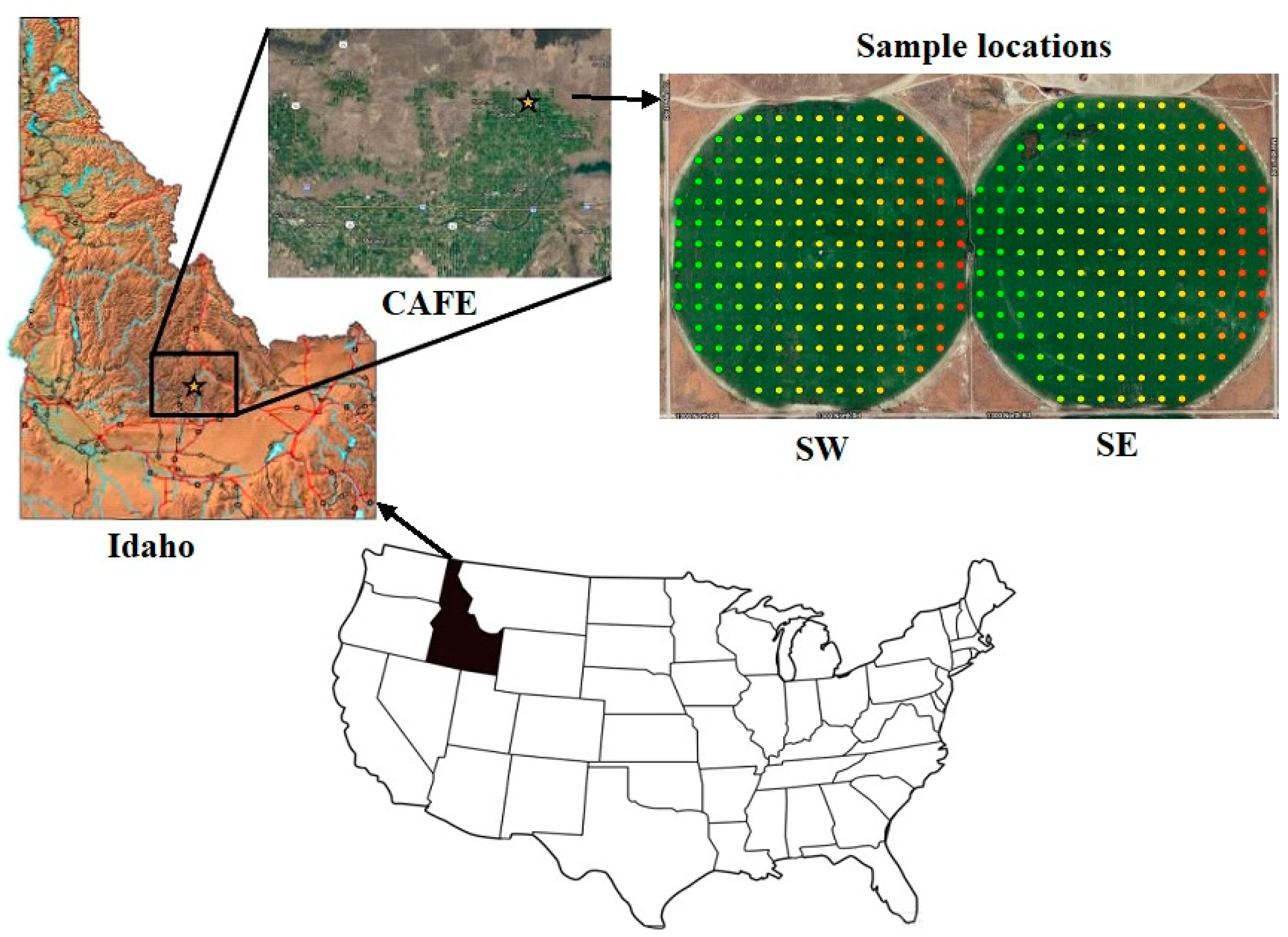
2.1. Study Area, Soil and Crop Yield Sampling, and Analysis

This research was conducted at two center pivot fields, denoted as the southeast field (SE) and southwest field (SW). Each field covered an area of approximately 52.6 ha. The SE and SW fields were situated within the confines of the Idaho Center for Agriculture, Food, and the Environment (Idaho CAFE) Sustainable Water and Soil Health Demonstration farm established in March of 2019, located near Rupert, ID, USA (48 48 28 N 113 40 5 W) (Figure 1). Prior to and after this date, the farm was managed by a commercial producer. The elevation of the site ranged from 1309 to 1331 amsl. This region experiences a semi-arid climate characterized by an annual precipitation of approximately 248 mm, with annual minimum, maximum, and average temperatures of 0 °C, 15.6 °C, and 7.8 °C, respectively (source: https://www.usclimatedata.com/climate/rupert/idaho/united-states/usid0223, accessed on 4 January 2024). The soils were classified as Minveno silt loam (loamy, mixed, superactive, mesic, shallow Xeric Haplodurids), Sluka silt loam (coarse-silty, mixed, superactive, mesic Xeric Haplodurids), and Power silt loam (fine-silty, mixed, superactive, mesic Xeric Calciargids). Historically, the cropping system employed at Idaho CAFE followed a four-year crop rotation cycle, including sugar beets (Beta vulgaris), barley (Hordeum vulgare), and potato (Solanum tuberosum), with uniform inorganic fertilizer applications. In 2019 and 2020, the fields were cultivated with barley and sugar beets, respectively. The fields underwent vertical tilling in the fall of 2019 and were roller harrowed in the following spring. Fertilization was carried out in both fields in the spring of 2020, with application rates of 247 kg N-ha⁻¹, 247 kg P-ha⁻¹, 185 kg K-ha⁻¹, and 10 kg Zn-ha⁻¹.

The SW field’s characterization was performed following the barley harvest in 2019, while the SE field’s characterization was conducted before planting but after fertilization in late March 2020. Results from this study are confounded by the timing of soil sampling. The original intention was to sample both the SE and SW fields in the fall of 2019; however, the number of soil samples that needed to be collected, stored, and processed was staggering. Thus, only the SW field was sampled. Due to a warmer-than-average March, the commercial operator fertilized the field with N, P, K, and Zn and lightly harrowed before the SE field could be soil sampled. This limits the ability to compare the two fields to one another since the SE field has higher nutrient values. However, it is still possible to characterize spatial variability since the fertilizer was spread uniformly over the field, such that low fertility areas would still be relatively low. In addition, the majority of micronutrients (Ca, Mg, Fe, Mn, Cu, and B) were not included in the fertilizer blend.

Each field was subdivided into grids measuring 51.7 m by 51.7 m, resulting in a grid density of 180 and 187 georeferenced sampling points for the SW and SE fields, respectively (as depicted in Figure 1). At each sampling point, soil samples were collected at two depths: 0–10 cm and 10–20 cm. This study presents the average values obtained from the combined 0–20 cm depth. The geographical coordinates, encompassing longitude and latitude, were recorded for each sampling point using a handheld global positioning system (GPS). Subsequently, the soil samples were labeled, air-dried, ground, and passed through a 2 mm sieve (US no. 10, Fisher Scientific Co., Hampton, NH, USA) before undergoing analysis for soil chemical properties.

The analysis of soil properties was outsourced to a commercial laboratory, with the following methods employed for property determination:

Organic matter (OM) was assessed through the loss of weight on the ignition method [39]. Excess lime (Lime) was assessed through the quantitative determination of soil carbonates using the gravimetric loss of carbon dioxide after reaction with hydrochloric acid of soil carbonates [40]. Soil pH and EC were measured using a 1:1 soil-to-water ratio [41]. Inorganic soil N concentration was determined using the 2 mol L⁻¹ potassium chloride extraction method [42]. Available P was assessed using the method described by [43] for neutral and alkaline soils (pH > 6.5). Soil available K was extracted by 1 N ammonium acetate (pH 7.0) and estimated using flame photometry, following the approach of [44]. Calcium and Mg were evaluated using a neutral 1.0 M ammonium acetate solution, and inductively coupled plasma (ICP) analysis as per [45,46]. Zinc, Fe, Mn, Cu, and B were determined using the DTPA-Sorbitol extraction method, following [47]. Cation exchange capacity was calculated by summing the cation milliequivalents per 100 g (mEq 100 g⁻¹) of K, Mg, Ca, and sodium (Na) using a neutral 1.0 M ammonium acetate solution and analyzed via ICP. The comprehensive data set allowed for a thorough investigation of the soil properties within the SE and SW fields.

At the time of initial sampling, both fields were equipped with mid-elevation spray application irrigation systems and a low-elevation spray application irrigation system was installed in the SE field after planting in April 2020. Each field was irrigated the same, however. Additionally, both fields were managed the same for tillage, fertilizer, crop, and chemical applications. Sugar beets were planted in both fields in late March 2020 and harvested in early October; barley was planted in early April 2021 and harvested in early September. Barley and sugar beets were hand harvested less than one week prior to bulk harvest to determine crop yields. For barley, the entire aboveground biomass was collected from a total of 21 georeferenced sampling locations (3 m × 3 m) per field using hand clippers. The clipped biomass samples were placed in paper bags, air dried, then threshed to estimate grain yield. Sugar beets were harvested from a total of 21 georeferenced sampling locations per field (crop row length: 3.05 m; approximate area: 0.56 m²). The sugar beets were counted and weighed before and after their foliage (tops) was separated from the root.

2.2. Statistical and Geostatistical Analyses

Descriptive statistics for each soil chemical property, encompassing measures such as mean, minimum, maximum, standard deviation, skewness, and coefficient of variation (CV), were computed using the Statistical Product and Service Solutions (IBM SPSS 18.0 software). Additionally, exploratory analyses and normality assessments were conducted, employing quantile–quantile (Q-Q) plots, histograms, and skewness values. Notably, some sampling locations exhibited atypical values or outliers that deviated from the general data set pattern, which were addressed to ensure accurate decision making [24,38]. The presence of non-normally distributed data with atypical values can introduce distortion, violating the principles of geostatistical theory [48,49]. Consequently, all observations of non-normal variables were log transformed to approximate normality [34,38], with the subsequent back transformation of the data set variable performed to revert it to its original scale [50].

A correlation analysis was conducted among the soil properties utilizing R (R Core Team, 2022) version 4.1.1. The Pearson correlation coefficients were visualized with the corrplot package [51].

To assess the spatial variability of soil properties, the geostatistical analyst tool within ArcGIS 10.5 software was employed. The characterization of spatial variability involved the computation of semivariograms following the methods outlined by [52,53], as per Equation (1) presented below:

$$\widehat{\gamma }\left(h\right)=\frac{1}{2N\left(h\right)}{\sum }_{i=1}^{N\left(h\right)}{\left({Z(x}_i\right)-{Z(x}_i+h\left)\right)}^2$$

(1)

where $\widehat{\gamma }$(h) is the empirical semi-variogram value at the lag interval distance h; N(h) is the number of sample pairs within the lag interval distance h; and Z(x_i) and Z(x_i + h) are sample values at the two spatial locations x_i and x_i + h, respectively.

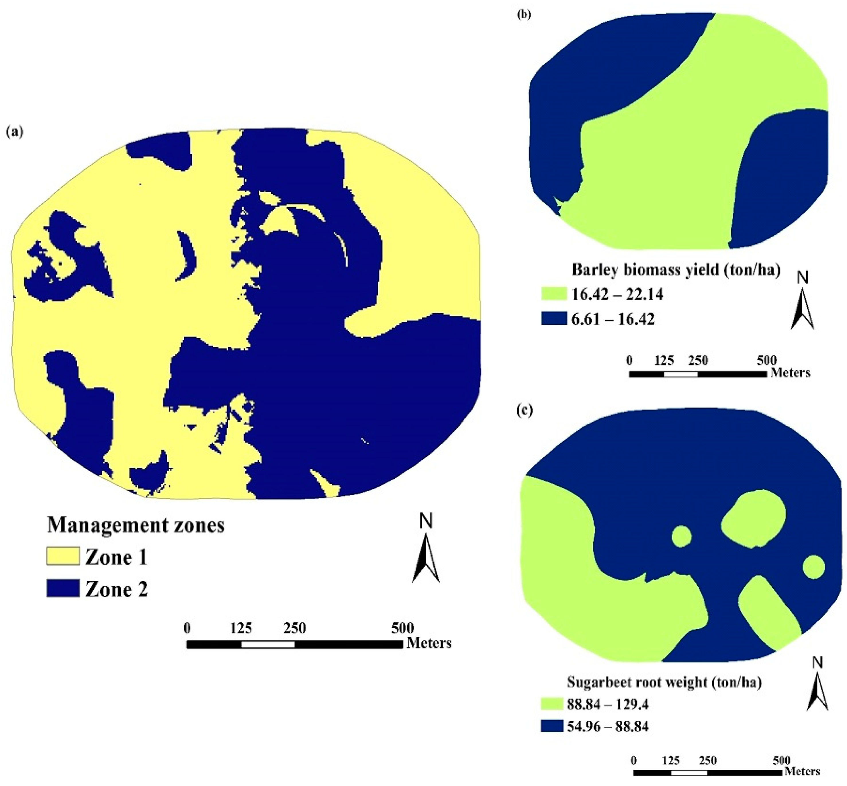
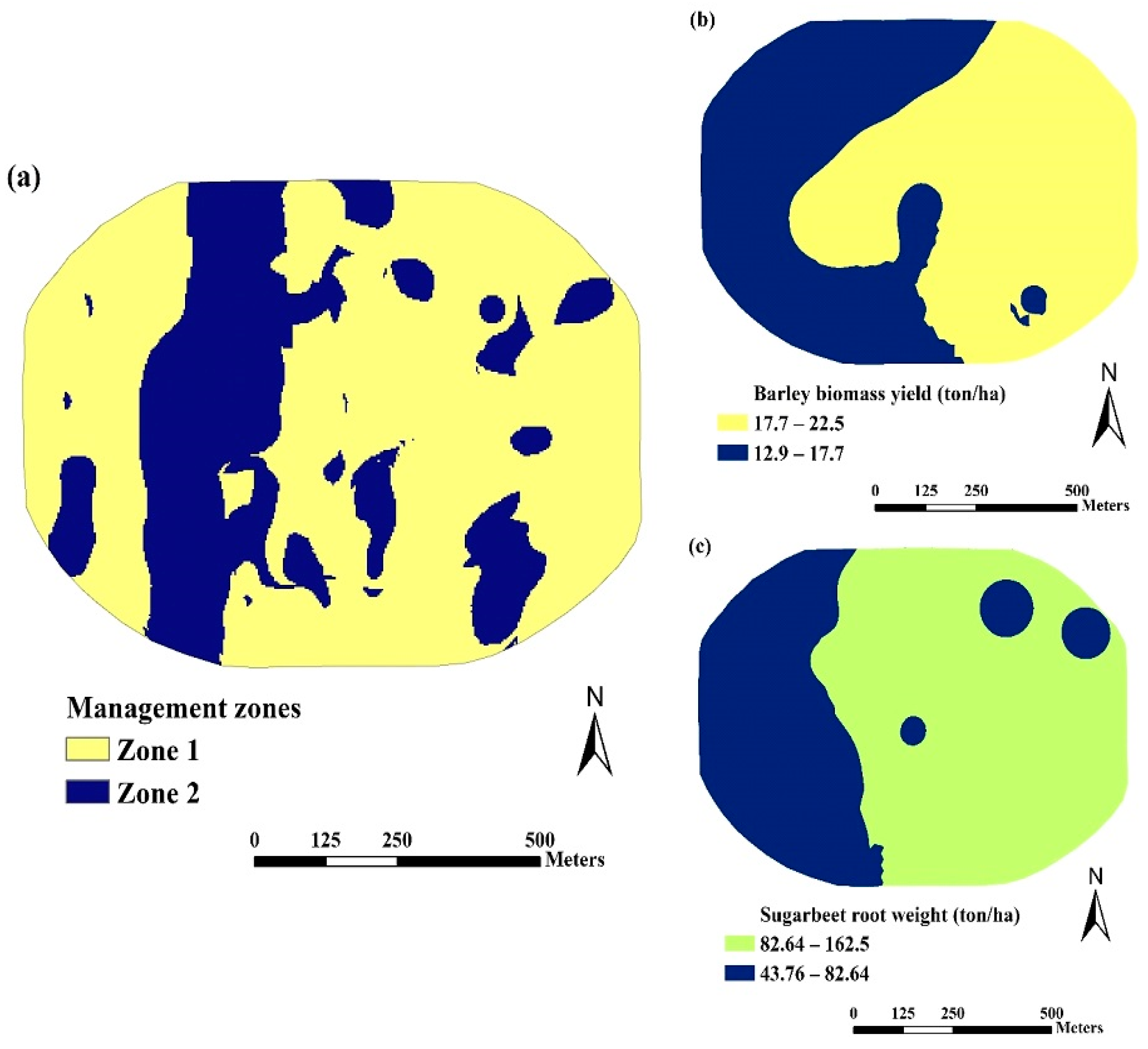
2.3. Mapping of Spatial Variability

The spatial variability of soil properties was assessed using the ordinary kriging interpolation method, a widely recognized technique for providing unbiased predictions for specific unsampled locations [54,55]. Various semivariogram models, including spherical, circular, exponential, stable, and K-Bessel, were examined to identify the best-fit model for each soil property. The accuracy of the spatial interpolation was assessed by employing a cross-validation approach using ArcGIS 10.5 software, where prediction errors such as mean error (ME) and root-mean-square standardized error (RMSSE) were calculated and compared [56]. An ME value near zero and an RMSSE value near one are indicative of a more accurate prediction model [57]. Nevertheless, it is worth noting that [58] highlighted that prediction accuracy can still be maintained even when RMSSE deviates from 1, as long as it falls within the tolerance interval of 1 + 3$\sqrt{2/N}$; 1 − 3$\sqrt{2/N}$. As per the methods proposed by [59,60], the ME and RMSSE were computed using the following formulas:

$$\mathrm{M}\mathrm{E}=\frac{1}{N}{\sum }_{i=1}^n(Z_i-Z_i\ast )$$

(2)

$$\mathrm{R}\mathrm{M}\mathrm{S}\mathrm{S}\mathrm{E}=\sqrt{\frac{1}{N}{\sum }_{i=1}^n\frac{{(Z_i-Z_i\ast )}^2}{\sigma i}}$$

(3)

where N represents the number of active observations, $Z_i$ is the observed value, $Z_i\ast$ is the estimated value, and σ is the kriging standard deviation.

The parameters of the geostatistical model, particularly the variance of the nugget-to-sill ratio, were employed to classify the spatial dependence of soil properties into distinct classes [38]. If the nugget-to-sill ratio is less than or equal to 25%, it indicates strong spatial dependency; if the ratio falls between 25% and 75%, it suggests moderate spatial dependency; and if the ratio exceeds or equals 75%, it implies weak spatial dependency [61].

2.4. Multivariate Analysis and Delineation of Management Zones

The PCA was conducted using the IBM SPSS 18.0 statistical software. Among the numerous PCs, those with eigenvalues greater than or equal to 1 were considered to explain the variance within the entire data set and to facilitate the development of MZ classes [30,60,62,63]. The highest factor loadings were considered the most representative of system variables [22]. In cases where multiple soil variables exhibited high factor loadings within a principal component (PC), correlation analysis was employed to eliminate redundant variables and select the most crucial soil property based on the correlation coefficient and system knowledge [64,65]. Consequently, key soil properties that explained the maximum variability were screened for the MDS [22].

The fuzzy K-means clustering algorithm was utilized to partition the field into distinct MZs. The fuzzy K-means aims to maximize the among-group variability while minimizing the within-group variability statistically, thus creating homogeneous groups [63].

The optimal number of clusters was determined using the R software, considering 17 clustering validity indices included in the R package Nbclust [66]. This package encompasses various indices that incorporate information regarding inter-cluster separation and intra-cluster compactness, thereby providing insights into the multivariate variability both between and within groups. Furthermore, it offers the user the best clustering scheme among different results [66,67]. The synthetic variables derived from the PCs were employed as input variables in the fuzzy K-means cluster analysis [67]. These analyses were performed on standardized values to mitigate the influence of different measurement units on the determination of soil attributes, with the data subsequently reverted to its original values for reporting [62,68]. This method is commonly used to identify MZs in precision agriculture research [69].

3. Results and Discussion

3.1. Overall Variability of Soil and Crop Parameters

The descriptive statistics of the measured soil chemical properties and crop yields in both the SE and SW fields are presented in

Table 1. Descriptive statistics of soil properties and crop yields in the SE and SW fields.

Soil Properties	SE (n = 187)							SW (n = 180)
	Mean	Min	Max	SD	Skewness	Skewness a	CV (%)	Mean	Min	Max	SD	Skewness	Skewness a	CV (%)
OM (%)	2.10	1.54	2.78	0.19	0.39	-	9.21	2.10	1.71	2.57	0.16	0.37	-	7.75
pH	7.89	6.85	8.40	0.26	−1.27	0.77	3.28	8.11	7.80	8.35	0.11	−0.17	-	1.40
CEC (meq 100 g−1)	19.21	14.80	22.65	1.43	−0.64	-	7.43	17.40	8.00	21.90	2.95	−1.23	−0.06	16.94
Excess lime (%)	2.93	0.00	12.55	2.34	1.63	0.30	79.90	4.03	1.00	8.95	1.81	0.72	-	44.90
EC (dS m−1)	1.41	0.85	3.34	0.44	1.84	0.87	31.11	1.58	0.95	3.60	0.44	1.52	0.73	28.00
T.I.N (kg ha−1)	42.96	17.64	98.49	15.73	0.90	-	36.62	16.16	8.59	35.12	3.65	2.36	0.75	22.59
P (kg ha−1)	67.59	25.09	248.7	25.42	2.61	0.52	37.61	28.82	15.73	50.49	6.21	0.67	-	21.57
K (kg ha−1)	309.7	171.7	668.9	106.9	1.73	0.88	34.52	164.8	63.9	380.6	51.6	0.81	-	31.32
Ca (kg ha−1)	19.90	15.52	22.77	1.70	−0.63	-	8.56	14.94	7.10	19.09	2.53	−1.13	−0.05	16.97
Mg (kg ha−1)	7.58	4.86	14.14	0.99	1.36	0.15	13.06	5.49	2.25	7.17	0.99	−1.13	0.22	18.08
Zn (kg ha−1)	5.13	2.65	10.79	1.28	1.47	0.52	24.88	2.25	1.25	4.14	0.68	0.89	-	30.12
Fe (kg ha−1)	8.37	3.74	19.26	3.06	1.15	0.33	36.53	6.20	3.83	12.18	1.27	1.39	0.38	20.45
Mn (kg ha−1)	7.35	3.49	13.36	1.90	0.75	-	25.93	3.17	1.98	5.13	0.67	0.56	-	21.16
Cu (kg ha−1)	1.45	0.61	2.63	0.30	0.66	-	20.75	1.40	0.7	2.73	0.36	1.01	0.04	25.59
B (kg ha−1)	1.54	0.56	2.86	0.41	−0.03	-	35.06	1.49	0.87	2.96	0.37	1.30	0.70	24.99
Crop yields (ton ha−1)
Barley grain	5.70	1.56	7.21	1.37	−1.78	0.54	24.01	6.08	3.81	7.97	1.22	−0.64	-	20.06
Barley biomass *	16.70	6.61	22.14	3.89	−1.08	−0.91	23.09	17.58	12.89	22.47	2.82	−0.02	-	16.05
Sugar beets root	86.05	54.96	129.4	18.16	0.31	-	21.10	83.51	43.76	162.5	25.26	1.5	0.75	30.25
Sugar beets biomass *	31.89	16.01	66.70	12.18	1.36	0.74	38.20	31.99	12.01	77.37	14.91	1.8	0.89	46.62

^a Skewness values after log transformation process. * The aboveground biomass. n: number of soil samples, OM: Organic Matter, CEC: Cation Exchange Capacity, EC: Electrical Conductivity, T.I.N: Total Inorganic Nitrogen, P: Phosphorus, K: Potassium, Ca: Calcium, Mg: Magnesium, Zn: Zinc, Fe: Iron, Mn: Manganese, Cu: Copper, B: Boron, Min: minimum, Max: maximum, SD: standard deviation, CV: coefficient of variation.

. The soils in both fields exhibit characteristics of alkalinity (pH > 7.3), low organic matter (OM < 2.5% by weight, in accordance with [70]), and low salinity (EC < 4 dS m⁻¹). The mean values and standard deviations for soil pH were 7.89 ± 0.26 and 8.11 ± 0.11, for OM were 2.10 ± 0.19 and 2.10 ± 0.16% in the SE and SW fields, respectively, and for soil EC were 1.41 ± 0.44 and 1.58 ± 0.44 dS m⁻¹ in the SE and SW fields, respectively. Additionally, the concentrations of soil total inorganic nitrogen (T.I.N), P, and K were higher in the SE field than in the SW field by 27, 39, and 145 kg ha⁻¹, respectively. This difference can be attributed to fertilization practices, as the SE field was fertilized prior to soil sampling.

The mean values and standard deviations for barley aboveground biomass yields were 16.70 ± 3.89 and 17.58 ± 2.82 ton ha⁻¹ in the SE and SW fields, respectively. For sugar beet root weight, the mean values and standard deviations were 86.05 ± 18.16 and 83.51 ± 25.26 ton ha⁻¹ in the SE and SW fields, respectively.

In analyzing the presented statistical data, the coefficient of variation (CV) emerges as a critical factor for characterizing data variability [31]. As per the criteria proposed by [71], soil variability is categorized as low (CV < 15%), moderate (15% < CV < 35%), or high (CV > 35%). Accordingly, excess lime, T.I.N, P, Fe, and B in the SE field and excess lime in the SW field exhibit high heterogeneity (CV > 35%) (Table 1). The heterogeneity in some soil chemical properties may be attributed to non-uniform fertilizer application, soil erosion, and irregular plant nutrient uptake due to other factors such as rooting depth and water stress [31]. In contrast, the other soil properties exhibit relatively low to moderate CV values in both fields. For example, soil pH displays low heterogeneity with CV values of 3.28 and 1.40% in the SE and SW fields, respectively. Previous research [38,72,73,74] has reported relatively small variations in the pH of the surface layer, with CV values ranging from 2.22% to 8.1%.

The CV values for soil OM are only 9.21 and 7.75% in the SE and SW fields, respectively. Soil OM is typically considered a relatively stable variable with minimal variation. However, the variability in soil OM content may be influenced by pedogenic processes shaped by micro-topographical variations [75]. This relatively stable and minimally variable nature of soil pH and OM is advantageous for organic matter management [31].

Soil available K, Zn, Mn, and Cu in both the SE and SW fields exhibit moderate heterogeneity. For example, the CV values for K are 34.52 and 31.32% in the SE and SW fields, respectively, aligning with the results of [31] who also reported a CV value of 34% for K.

The sugar beets aboveground biomass exhibits high heterogeneity, with CV values of 38.20% and 46.62% in the SE and SW fields, respectively. In contrast, the barley aboveground biomass shows moderate heterogeneity, with CV values of 23.09% and 16.05% in the SE and SW fields, respectively (Table 1).

The normality of data distribution was assessed using Q-Q plots, histograms, and skewness values. The soil OM, CEC, T.I.N, Ca, Mn, Cu, and B in the SE field, and soil OM, pH, excess lime, P, K, Zn, and Mn in the SW field were found to be normally distributed. For non-normally distributed data, a log transformation was applied to normalize or approximate a normal distribution and reduce skewness values (Table 1). A data set with high skewness values (>±1) has been shown to negatively impact spatial structure [49], and log transformation is commonly employed to approximate normality [31,34].

The pronounced variation of soil K in the SE field and soil T.I.N in the SW field indicates high skewness values, largely attributed to extreme K and T.I.N values from a few samples (three and two samples, respectively), which could be considered outliers. These findings are consistent with those of other researchers [38,76], who have reported elevated K values in soils due to the presence of unweathered biotites in clay and silt size fractions, releasing substantial amounts of K [77]. After removing the outliers and applying logarithmic (log) transformations, the skewness values for K and T.I.N were notably reduced in both fields (Table 1). The presence of outliers in the data set can disrupt the structure of semivariograms and violate geostatistical theory, as noted by [48,78]. Consequently, in this study, the outlier values were replaced by the maximum values for soil K and T.I.N in the SE and SW fields, respectively, as outliers can distort variograms in the kriging analysis.

The Pearson correlation coefficients, depicting the relationships among the studied soil chemical properties in the SE and SW fields, are illustrated in Figure 2a,b, with the size of the circle indicating the strength of correlation (red represents negative correlation, while blue represents positive correlation). Strong positive correlations were observed between soil EC and T.I.N, as well as between CEC and Ca. Furthermore, moderate positive correlations were found between soil OM and K, EC and Zn, and EC and B in both fields. This is likely attributed to the fact that soil EC indirectly measures several soil properties that influence soil fertility. Soil OM, on the other hand, influences soil chemical, physical, and biological properties, affecting nutrient and water availability to crops [30]. Strong negative correlations were found between Cu and B in both fields. Similar correlations are depicted in Figure 2, such as positive and negative correlations between soil pH and excess lime and Fe, respectively, in both fields. Positive and significant correlations were observed between Cu and Zn, as well as between Mn and Fe in both fields, indicating common sources of origin and factors influencing the availability and distribution of these cationic micro-nutrients [79]. In alignment with the findings of the present study, Ref. [80] also reported positive correlations among the cationic micro-nutrients.

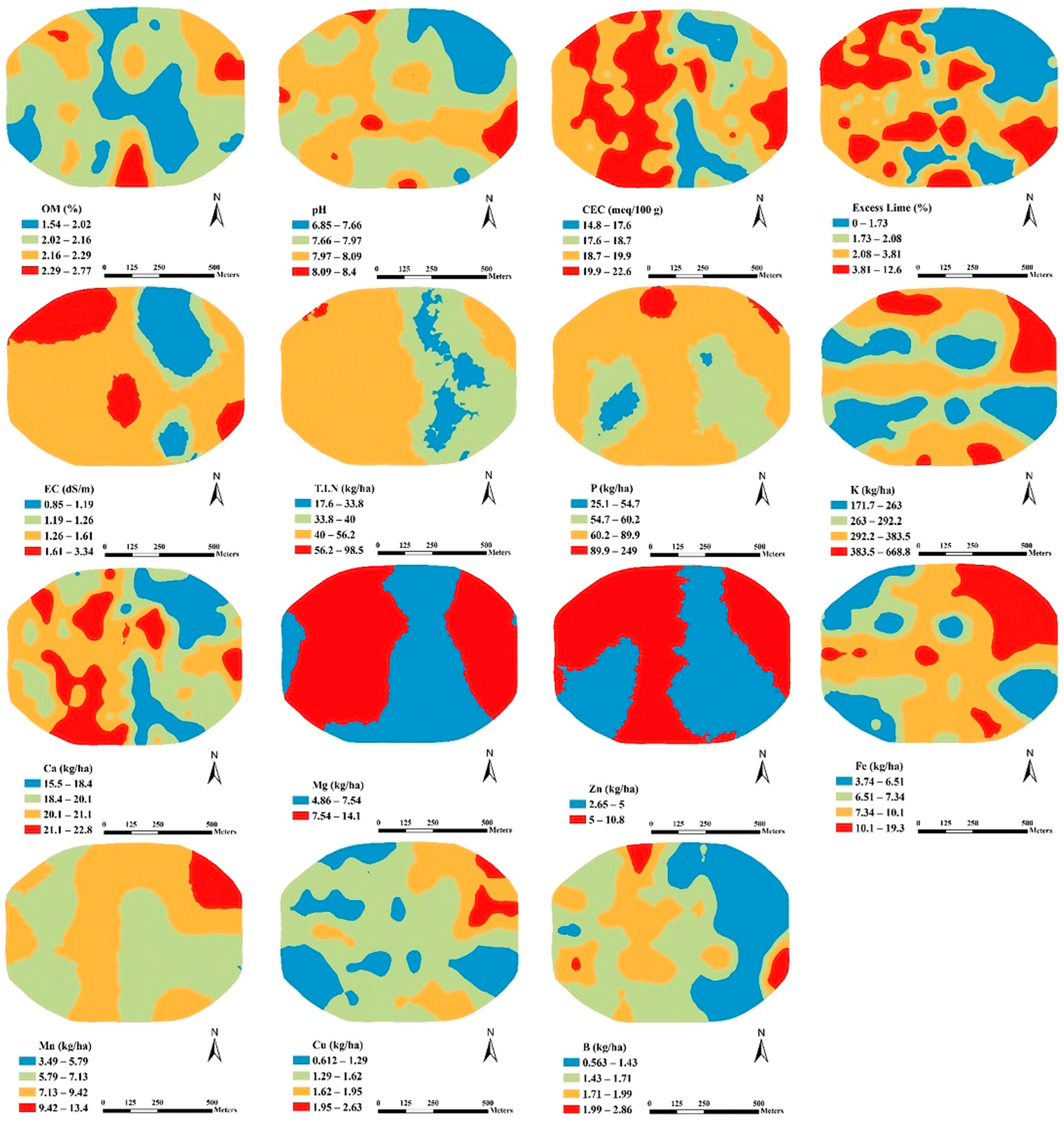
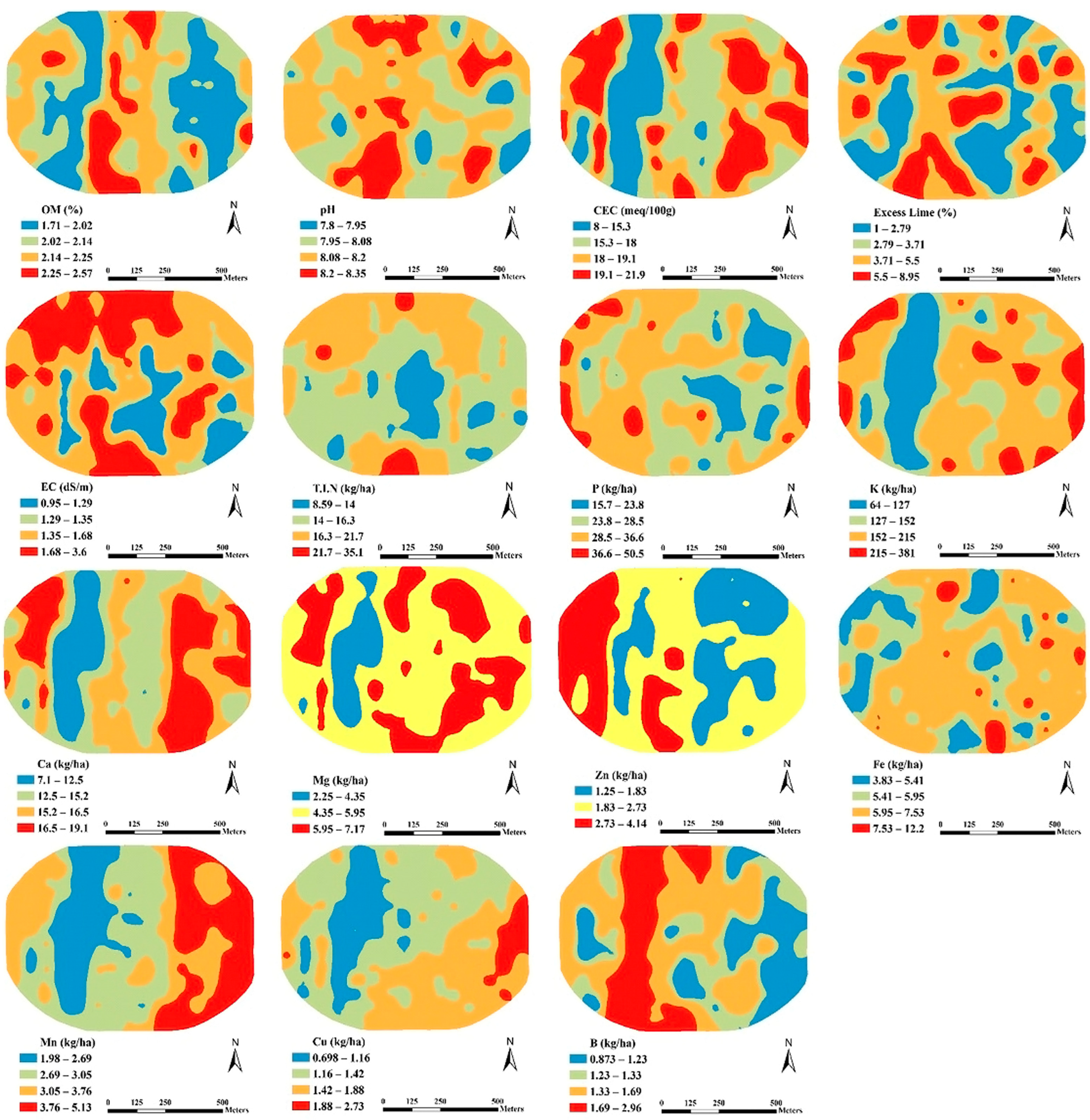
3.2. Spatial Variability of Soil Properties

Based on the evaluation of prediction errors (ME and RMSSE), the best-fitted models obtained through semivariogram analysis for various soil properties and their degree of spatial dependence are presented in

Table 2. Semivariogram parameters of the soil properties in the SE field.

Soil Properties	Model	Nugget	Partial Sill	Sill	Nugget/ Sill (%)	SDC	ME	RMSSE
OM (%)	Spherical	0.02	0.02	0.04	46.19	Moderate	0.00	1.00
pH	Spherical	0.02	0.04	0.06	27.99	Moderate	0.00	1.05
CEC (meq 100 g−1)	Exponential	0.00	1.68	1.68	0.00	Strong	−0.01	1.15
Excess lime (%)	Exponential	0.01	5.20	5.21	0.25	Strong	−0.03	1.01
EC (dS m−1)	Circular	0.14	0.07	0.21	68.62	Moderate	0.00	1.00
T.I.N (kg ha−1)	Stable	198.54	74.96	273.50	72.59	Moderate	−0.13	1.01
P (kg ha−1)	Spherical	458.92	231.19	690.11	66.50	Moderate	−0.30	1.03
K (kg ha−1)	Spherical	4069.4	6413.7	10,483.1	38.82	Moderate	−0.61	1.00
Ca (kg ha−1)	K-Bessel	0.00	2.95	2.95	0.00	Strong	−0.01	1.02
Mg (kg ha−1)	K-Bessel	0.67	0.39	1.06	63.08	Moderate	0.00	1.06
Zn (kg ha−1)	Stable	1.41	0.27	1.68	83.91	Weak	−0.02	1.01
Fe (kg ha−1)	Exponential	3.80	5.61	9.41	40.38	Moderate	0.01	0.97
Mn (kg ha−1)	Stable	2.39	1.25	3.64	65.74	Moderate	0.00	1.03
Cu (kg ha−1)	Exponential	0.02	0.07	0.08	19.78	Strong	0.00	1.01
B (kg ha−1)	Spherical	0.04	0.09	0.13	29.28	Moderate	−0.01	1.02

OM: Organic Matter, CEC: Cation Exchange Capacity, EC: Electrical Conductivity, T.I.N: Total Inorganic Nitrogen, P: Phosphorus, K: Potassium, Ca: Calcium, Mg: Magnesium, Zn: Zinc, Fe: Iron, Mn: Manganese, Cu: Copper, B: Boron, SDC: spatial dependency class, ME: mean error, RMSSE: root-mean-square standardized error.

and

Table 3. Semivariogram parameters of the soil properties in the SW field.

Soil Properties	Model	Nugget	Partial Sill	Sill	Nugget/ Sill (%)	SDC	ME	RMSSE
OM (%)	Exponential	0.00	0.03	0.03	0.02	Strong	0.00	0.96
pH	Stable	0.00	0.01	0.01	0.00	Strong	0.00	1.00
CEC (meq 100 g−1)	Exponential	0.00	9.17	9.18	0.05	Strong	0.00	0.91
Excess lime (%)	Exponential	0.00	3.67	3.67	0.00	Strong	0.00	0.96
EC (dS m−1)	Exponential	0.01	0.19	0.20	2.79	Strong	0.00	0.98
T.I.N (kg ha−1)	K-Bessel	0.00	12.46	12.46	0.00	Strong	−0.01	1.03
P (kg ha−1)	Exponential	0.03	34.56	34.59	0.10	Strong	−0.18	0.91
K (kg ha−1)	Exponential	0.00	2447.6	2447.6	0.00	Strong	−1.08	0.97
Ca (kg ha−1)	Exponential	0.00	6.61	6.61	0.00	Strong	0.00	0.76
Mg (kg ha−1)	Exponential	0.00	1.05	1.05	0.00	Strong	0.01	0.82
Zn (kg ha−1)	Exponential	0.00	0.39	0.39	0.00	Strong	0.00	0.79
Fe (kg ha−1)	Exponential	0.00	1.56	1.56	0.00	Strong	0.01	1.01
Mn (kg ha−1)	Exponential	0.00	0.57	0.57	0.00	Strong	0.00	1.01
Cu (kg ha−1)	Exponential	0.00	0.05	0.05	0.00	Strong	0.00	0.98
B (kg ha−1)	Exponential	0.00	0.17	0.17	0.00	Strong	0.00	0.89

OM: Organic Matter, CEC: Cation Exchange Capacity, EC: Electrical Conductivity, T.I.N: Total Inorganic Nitrogen, P: Phosphorus, K: Potassium, Ca: Calcium, Mg: Magnesium, Zn: Zinc, Fe: Iron, Mn: Manganese, Cu: Copper, B: Boron, SDC: spatial dependency class, ME: mean error, RMSSE: root-mean-square standardized error.

, and (Supplementary Figures S1 and S2). In the SE field, the best-fit model for soil OM, pH, P, K, and B was determined to be spherical. Excess lime, CEC, Fe, and Cu exhibited an exponential best-fit model, while soil T.I.N, Zn, and Mn displayed a stable best-fit model. Additionally, soil EC and Ca demonstrated circular and K-Bessel best-fit models, respectively (Table 3). These findings are consistent with previous studies that reported the prevalence of exponential, stable, K-Bessel, and spherical best-fit models for soil chemical properties [81,82,83]. In the SW field, exponential models were the best-fitted models for most soil properties, with the exception of soil pH and T.I.N, for which stable and K-Bessel models were more appropriate, as shown in Table 3.

In both the SE and SW fields, most soil properties exhibited ME and RMSSE values close to zero and one, respectively, indicating that kriging predictions for unsampled soil property values closely aligned with the measured values.

The nugget values, which provide insights into micro-variability, were generally small for most soil properties (ranging from 0 to 3.8) in the SE field (Table 2). However, soil T.I.N, P, and K showed larger nugget values (ranging from 198.54 to 4069.4). This aligns with previous research by [30] in India, who also recorded small nugget values (ranging from 0 to 0.78) for soil pH, EC, and soil organic carbon (SOC) but larger values (ranging from 67.4 to 64,136.1) for soil P and K. These large nugget values suggest a more substantial influence of ecological processes over small scales, indicating that the selected sampling distances might not adequately capture the spatial dependence. The sill values, which represent the variance of the sampled population at large separation distances, were also higher for soil T.I.N, P, and K in both fields. These variations in nugget and sill values for certain soil properties align with the observations made by [83,84].

Based on the nugget-to-sill ratio, the spatial dependence of the studied soil properties exhibited variation. In the SW field, all soil properties, as well as soil Ca, excess lime, CEC, and Cu in the SE field, displayed strong spatial dependence (≤25%) (Table 2 and Table 3). However, in the SE field, Zn exhibited weak spatial dependence (83.91%), while other soil properties showed moderate spatial dependence (ranging from 29.28 to 72.59%). The strong spatial dependence observed in this study is largely attributed to geomorphological and soil structural factors, including parent material, depth to bedrock, topography, and soil texture. In contrast, weaker spatial dependence on soil properties is influenced by extrinsic random factors such as climatic conditions, land use changes, and soil management practices (i.e., fertilization, tillage, and the uniformity of the irrigation system). The moderate spatial dependence can be attributed to a combination of both soil structural and extrinsic factors, which may be related to leaching processes [30].

The spatial distribution maps of soil properties, generated through ordinary kriging interpolation, are presented in Figure 3 and Figure 4. In the SE field (Figure 3), it is evident that lower soil OM values (ranging from 1.54 to 2.02%) are concentrated in the central region, while higher soil OM values (ranging from 2.29 to 2.77%) are found in the southern part. The soil pH distribution is opposite to that of Fe, especially in the northeast part of the field, consistent with a negative correlation between soil pH and Fe. Soil T.I.N and P exhibit values in the range of 40–52.2 kg ha⁻¹ and 62.2–89.9 kg ha⁻¹, respectively, across most of the area, with higher values in the north and northwest parts. Lower soil K values (ranging from 171.7 to 263 kg ha⁻¹) are primarily found in the middle of the field, while soil B is notably deficient in the eastern parts. Soil Mn is within a moderate range, with a few patches showing lower values in the eastern part. Soil Ca, Cu, CEC, and excess lime exhibit varying distribution patterns across the study area. The observed values of each soil property tend to be higher in the SE field compared to the SW field.

In the SW field (Figure 4), the mid-western portions of the study area have lower values for soil K, Ca, Mn, Mg, OM, CEC, and Cu, but higher values for soil B, likely due to a negative correlation with Cu. The highest soil pH and EC values were concentrated in the northern and southern parts, ranging from 8.2–8.35 and 1.68–3.6 dS m⁻¹, respectively, indicating alkaline soils with no salinity issues (EC < 4 dS m⁻¹). The study area generally has low soil OM content (<2.5%). Soil T.I.N, P, and K exhibit considerable variation, with low soil T.I.N values ranging from 14 to 16.3 kg ha⁻¹ in large areas, while soil P and K fall mostly in the range of 28.5–36.6 kg ha⁻¹ and 152–215 kg ha⁻¹, respectively. The high spatial variations in nutrient availability over short distances likely contribute to the high coefficient of variation for T.I.N, P, and K, consistent with the results obtained by [55] in China. In the present study, the higher variability in soil T.I.N is linked to soil alkalinity, low OM content, suboptimal management practices, and mineralization. In contrast, the dominance of potassium-rich minerals and soil management practices results in variations in K and p values [31].

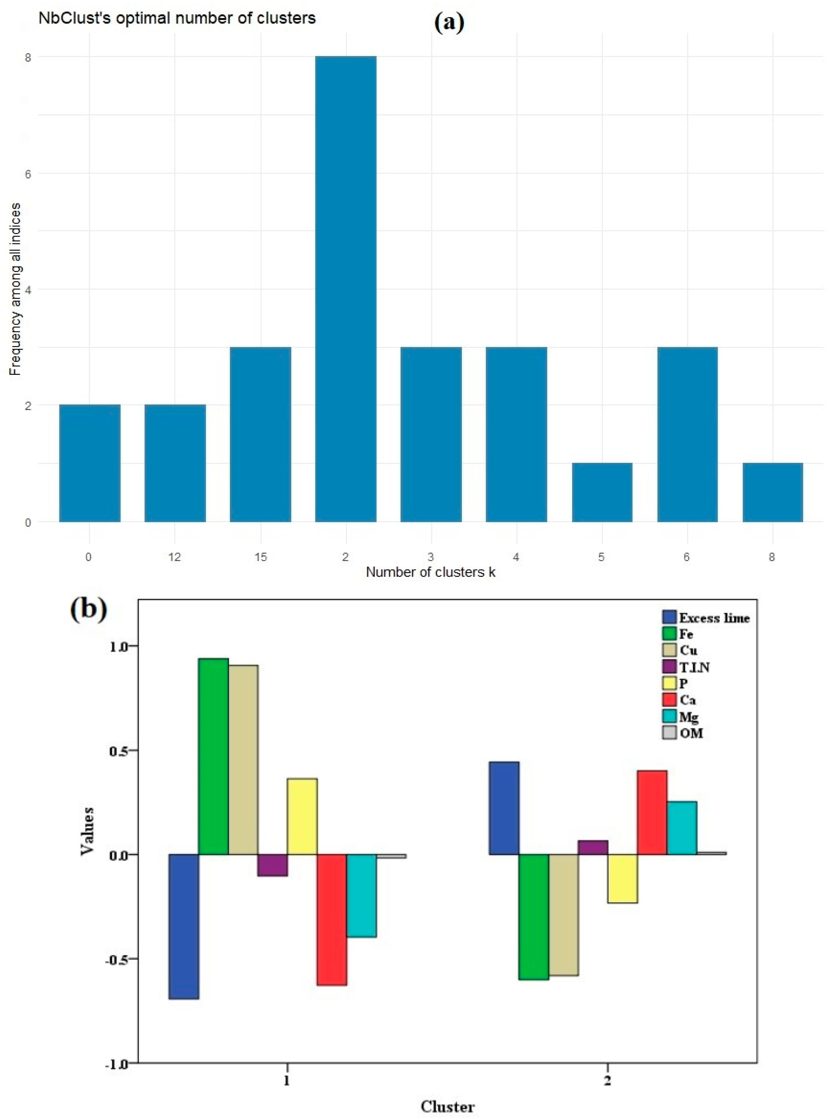
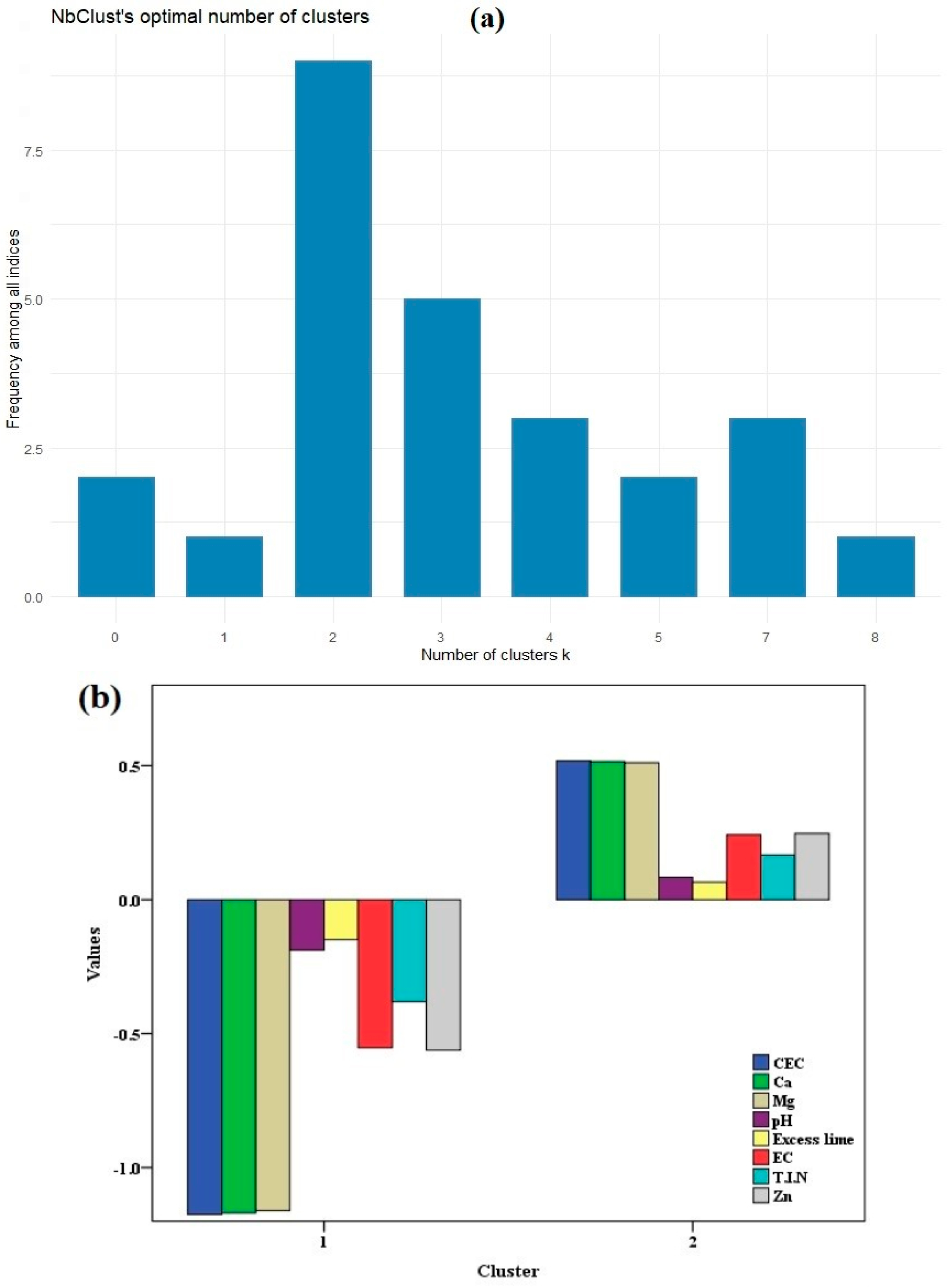
3.3. Multivariate Analysis and Delineation of Management Zones

To ensure a meaningful representation of the data, the PCs with eigenvalues greater than or equal to 1.0 were retained. In the SE field (

Table 4. Principal component analysis of soil properties and loading coefficient for the first five principal components in the SE field.

PCs	PC1	PC2	PC3	PC4	PC5
Eigenvalue	4.34	3.09	2.06	1.37	1.17
Variance (%)	28.93	20.62	13.75	9.11	7.82
Cumulative variability (%)	28.93	49.55	63.30	72.41	80.23
Principal component loading for each variable
OM (%)	0.07	0.09	−0.01	−0.05	0.96
pH	−0.77	−0.09	0.42	−0.16	−0.03
CEC (meq 100 g−1)	−0.15	0.12	0.85	0.47	0.00
Excess lime (%)	−0.82	0.07	−0.01	−0.03	0.31
EC (dS m−1)	−0.33	0.78	0.01	0.09	0.16
T.I.N (kg ha−1)	−0.10	0.84	0.12	0.08	0.13
P (kg ha−1)	0.30	0.83	−0.05	−0.13	−0.12
K (kg ha−1)	0.67	0.44	0.03	−0.18	0.17
Ca (kg ha−1)	−0.19	0.10	0.95	0.01	0.00
Mg (kg ha−1)	−0.04	−0.09	0.20	0.94	−0.06
Zn (kg ha−1)	0.28	0.73	0.23	−0.21	−0.05
Fe (kg ha−1)	0.84	0.09	−0.17	−0.02	−0.04
Mn (kg ha−1)	0.61	0.49	−0.20	0.28	0.04
Cu (kg ha−1)	0.89	−0.02	0.01	−0.16	0.18
B (kg ha−1)	−0.63	0.28	0.28	0.18	−0.18

Bold-underlined values indicate the highest factor loading for each PC and, therefore, the properties selected as the best for inclusion in the MDS. PC: principal component, OM: Organic Matter, CEC: Cation Exchange Capacity, EC: Electrical Conductivity, T.I.N: Total Inorganic Nitrogen, P: Phosphorus, K: Potassium, Ca: Calcium, Mg: Magnesium, Zn: Zinc, Fe: Iron, Mn: Manganese, Cu: Copper, B: Boron.

), the first five PCs, collectively accounting for 80.23% of the cumulative variance in the data set, were selected for subsequent analysis. Upon assessing variable loadings, the highly weighted variables were prioritized.

The first principal component (PC1) explained 28.93% of the total variance, with a primary influence from Cu, Fe, and excess lime. The second principal component (PC2) was predominantly shaped by T.I.N and P, explaining 20.62% of the total variance. PC3, the third principal component, accounted for 13.75% of the total variance and featured a pronounced presence of Ca and CEC, with Ca exhibiting a particularly high correlation with CEC. Consequently, the highest weighted value of Ca (0.95) was retained in PC3. The fourth principal component (PC4) was uniquely characterized by Mg, explaining 9.11% of the total variance. Lastly, the fifth principal component (PC5) contributed an additional 7.82% to the total variance, primarily driven by soil OM.

In the SW field, the first four PCs exhibited eigenvalues greater than or equal to 1, collectively contributing to a cumulative variability of 71.15% (

Table 5. Principal component analysis of soil properties and loading coefficient for the first four principal components in the SW field.

PCs	PC1	PC2	PC3	PC4
Eigenvalue	4.56	2.35	1.94	1.83
Variance (%)	30.42	15.64	12.90	12.20
Cumulative variability (%)	30.42	46.06	58.96	71.15
Principal component loading for each variable
OM (%)	0.14	0.31	0.06	0.59
pH	−0.01	0.78	−0.09	0.09
CEC (meq 100 g−1)	0.94	0.10	0.18	0.18
Excess lime (%)	−0.02	0.77	0.16	0.10
EC (dS m−1)	0.14	0.23	0.87	0.15
T.I.N (kg ha−1)	0.08	−0.06	0.89	0.07
P (kg ha−1)	−0.28	−0.46	0.06	0.72
K (kg ha−1)	0.64	−0.31	−0.06	0.49
Ca (kg ha−1)	0.95	0.08	0.12	0.14
Mg (kg ha−1)	0.90	0.15	0.25	0.04
Zn (kg ha−1)	0.27	0.08	0.19	0.74
Fe (kg ha−1)	0.16	-.047	−0.12	0.09
Mn (kg ha−1)	0.77	−0.36	−0.06	−0.08
Cu (kg ha−1)	0.62	−0.41	−0.05	0.21
B (kg ha−1)	−0.62	0.35	0.42	0.12

Bold-underlined values indicate the highest factor loading for each PC and, therefore, the properties selected as the best for inclusion in the MDS. PC: principal component, OM: Organic Matter, CEC: Cation Exchange Capacity, EC: Electrical Conductivity, T.I.N: Total Inorganic Nitrogen, P: Phosphorus, K: Potassium, Ca: Calcium, Mg: Magnesium, Zn: Zinc, Fe: Iron, Mn: Manganese, Cu: Copper, B: Boron.

). The first PC, accounted for 30.42% of the total variance and displayed high positive loadings for Ca (loading = 0.95), CEC (loading = 0.94), and Mg (loading = 0.90). The second PC explained 15.64% of the total variance and exhibited positive loadings for soil pH (loading = 0.78) and excess lime (loading = 0.77). The third PC accounted for 12.90% of the total variance and was characterized by high positive loadings for soil T.I.N (loading = 0.89) and EC (loading = 0.87). Finally, the fourth PC explained 12.20% of the total variance and was primarily defined by Zn (loading = 0.74).

To summarize, in the SE and SW fields, the PCA amalgamated the eight investigated soil properties into five and four PCs, respectively, effectively encapsulating the majority of spatial variability. These findings align with previous research by [85,86], who similarly reported four and five PCs derived from PCA, effectively summarizing the variability of soil properties.

In order to delineate site-specific management zones, it is helpful to establish in advance the optimal number of clusters for partitioning. The variables derived from PCs were subsequently utilized as input parameters in the fuzzy k-means clustering analysis. In this study, we applied the methodology introduced by [66], which involved utilizing multiple indices to ascertain the optimum number of clusters. As a result of the fuzzy k-means clustering analysis, two clusters were identified in both fields (Figure 5a and Figure 6a). The optimal number of clusters was determined based on the highest frequency among all the indices, as [66,67] recommended adopting the majority rule to determine the number of clusters after calculating various indices. The standardized values of the soil variables derived from PCs in the SE and SW fields are found in Figure 5b and Figure 6b. The graphical representation reveals unique and distinctive patterns within each cluster. For example, in the first cluster of the SW field, the standardized values for CEC, pH, T.I.N, and Zn were −1.17, −0.19, −0.38, and −0.56, respectively. Conversely, in the second cluster, these values were 0.52, 0.09, 0.17, and 0.25, respectively, indicating differences in the soil attributes between the clusters. Similar results have also been observed in the identification of two clusters in the delineation of soil properties and yield zones [86,87,88].

Using the spatial analysis tools within ArcMap, eight soil properties, which were determined as decisive factors through PCA for each field, were reclassified into two classes. These reclassifications included new preference values, and the resulting layers were employed as inputs in overlay operations. Reclassification processes are reorganizing existing information within a single map. Conversely, overlay operations are the integration of two or more maps and lead to the delineation of novel boundaries [89]. The weighted overlay tool was utilized to superimpose the raster maps representing soil properties. In this process, each input raster could be weighted, signifying its percentage of influence based on its significance. This percentage influence was determined by considering the percentage of variance accounted for by each principal component and the highest loading value associated with each variable.

The resulting maps revealed the presence of two distinct MZs in both fields, as depicted in Figure 7a and Figure 8a. For visual assessment and inspection, the ordinary kriging interpolation method was applied to create spatial variability maps, which were further classified into two categories for barley aboveground biomass yield and sugar beets root yield. This was carried out to assess whether these potential MZs corresponded to varying crop productivity levels within the SE and SW fields. The resulting maps related to yield productivity are also presented in Figure 7b,c and Figure 8b,c. The spatial distribution of barley and sugar beet yields appears to encapsulate the integrated information derived from the eight soil chemical attributes specific to each field. Additionally, the spatial distribution of yields in some areas exhibited a certain degree of similarity with the distribution of MZs. The results from this study are consistent with the findings of [68], which indicated that dividing the study area into two MZs struck a suitable balance between sensitivity and the visual variability patterns of soil properties and crop yields.

The mean values and standard deviations of soil properties and crop yields for the two distinct MZs within both the SE and SW fields are found in

Table 6. Mean values and standard deviations of soil properties and crop yields in different management zones.

SE Field			SW Field
Management Zones	Zone 1	Zone 2	Management Zones	Zone 1	Zone 2
n	102	85	n	118	62
Area (%)	51.8	48.2	Area (%)	72.4	27.6
Soil properties			Soil properties
OM (%)	2.14 ± 0.19	2.06 ± 0.19	pH	8.08 ± 0.10	8.14 ± 0.12
Excess lime (%)	2.51 ± 1.98	3.28 ± 2.56	CEC (meq 100 g−1)	18.67 ± 1.4	15.01 ± 3.6
T.I.N (kg ha−1)	48.96 ± 15.7	37.96 ± 13.9	Excess lime (%)	3.71 ± 1.5	4.65 ± 2.1
P (kg ha−1)	75.19 ± 30.3	61.25 ± 18.3	EC (dS m−1)	1.58 ± 0.43	1.59 ± 0.48
Ca (kg ha−1)	20.37 ± 1.46	19.51 ± 1.80	T.I.N (kg ha−1)	16.51 ± 3.9	15.50 ± 3.0
Mg (kg ha−1)	7.68 ± 0.81	7.49 ± 1.12	Ca (kg ha−1)	16.04 ± 1.2	12.85 ± 3.0
Fe (kg ha−1)	9.18 ± 3.45	7.69 ± 2.51	Mg (kg ha−1)	5.86 ± 0.52	4.77 ± 1.3
Cu (kg ha−1)	1.53 ± 0.33	1.38 ± 0.26	Zn (kg ha−1)	2.39 ± 0.75	1.98 ± 0.41
Crop yields (ton ha−1)			Crop yields (ton ha−1)
Barley grain	6.14 ± 0.66	5.43 ± 1.6	Barley grain	6.27 ± 1.1	5.78 ± 1.4
Barley biomass *	17.19 ± 2.8	16.40 ± 4.5	Barley biomass *	18.39 ± 2.9	16.69 ± 2.5
Sugar beet root	89.01 ± 12.3	84.23 ± 21.3	Sugar beet root	88.98 ± 31.9	77.43 ± 14.7
Sugar beet biomass *	36.68 ± 13.5	28.94 ± 10.8	Sugar beet biomass *	32.95 ± 12.3	30.92 ± 18.1

* The aboveground biomass, n: number of points, OM: Organic Matter, CEC: Cation Exchange Capacity, EC: Electrical Conductivity, T.I.N: Total Inorganic Nitrogen, P: Phosphorus, Ca: Calcium, Mg: Magnesium, Zn: Zinc, Fe: Iron, Cu: Copper.

. In the SE field, Zone 1 covered 51.8% of the geographical area, while Zone 2 constituted the remaining 48.2%. In the SW field, 72.4% of the area was in Zone 1, while the remaining 27.6% was in Zone 2.

Compared to Zone 2, Zone 1 in the SE field exhibited lower excess lime content and higher soil fertility potential due to higher values of soil OM, T.I.N, P, Ca, Mg, Fe, and Cu. Additionally, crop yields, including barley grain and biomass yields, and sugar beet root weight and biomass yields were also higher in Zone 1. For instance, the average soil OM content in Zone 1 was 2.14% compared to 2.06% in Zone 2. Excess lime in Zone 1 was 23.5% lower than that in Zone 2. Furthermore, the average T.I.N, P, and Fe mean values in Zone 1 exceeded those in Zone 2 by 22.5, 18.5, and 16.2%, respectively. Consequently, the biomass yields of barley and sugar beets in Zone 1 were 4.6% and 21.1% higher, respectively, compared to Zone 2.

In the SW field, Zone 2 displayed higher values of soil pH, excess lime, and EC, while Zone 1 exhibited greater soil fertility potential, as indicated by elevated values of T.I.N, CEC, Ca, Mg, and Zn. Similarly, crop yields were higher in Zone 1, with increased barley grain yield and sugar beet root weight, compared to Zone 2. For instance, the average pH and EC values in Zone 1 were 8.08 and 1.58 dS m⁻¹, whereas in Zone 2, they were 8.14 and 1.59 dS m⁻¹, respectively. Zone 1 had 20.2% lower excess lime content than Zone 2. The average values of T.I.N, Ca, and Zn in Zone 1 exceeded those in Zone 2 by 6.1, 19.9, and 17.2%, respectively. Evidently, barley grain yield and sugar beet root weight in Zone 1 were 7.8% and 13% higher, respectively, compared to Zone 2 in the SW field. The average values of soil properties offer a valuable reference for site-specific soil nutrient management through varied application rates [29,30]. To enhance soil quality, promote crop productivity, and prevent land degradation in the SE and SW fields, it is recommended to prioritize the augmentation of soil organic matter through the use of organic manure and the implementation of conservation agriculture practices.

4. Conclusions

In the semi-arid region of Southern Idaho, an extensive soil sampling campaign was conducted within fields that were utilized for the cultivation of barley and sugar beets in a crop rotation system. A total of 187 and 180 georeferenced soil samples were collected from the SE and SW fields, respectively. These samples underwent comprehensive analysis to determine key soil properties such as soil pH, EC, excess lime content, and the availability of essential macro and micronutrients. The soil characteristics in both fields were indicative of alkalinity, low organic matter content, and low salinity levels. Significant positive correlations were observed between soil EC and T.I.N, as well as between CEC and Ca. Conversely, strong negative correlations were detected between Cu and B in both fields. The coefficients of variation for soil chemical properties unveiled substantial spatial variability, underscoring the need for site-specific nutrient management practices in both fields. To assess the spatial variability of soil fertility properties, geostatistical methods were employed, and the data were clustered into two distinct soil management zones using principal component analysis (PCA) and a fuzzy k-means clustering classification approach. The geostatistical analysis identified the best-fit semivariogram models for the studied soil properties, including exponential, spherical, circular, K-Bessel, and stable models, highlighting the spatial heterogeneity with varying degrees of spatial dependence. The resulting two management zones, derived through PCA and fuzzy k-means clustering, exhibited significant differences in terms of the eight soil properties serving as decisive factors within each field. In general, the first management zone displayed lower values of soil pH, excess lime content, and soil EC, while concurrently demonstrating higher soil fertility potential compared to the second management zone in both fields. Consequently, higher crop productivity, specifically in barley and sugar beets, was achieved in the first management zone. By considering the average soil chemical properties within each management zone, farmers can effectively optimize their fertilizer applications, leading to improved agricultural practices. The establishment of soil management zones enables farmers to adopt precision agriculture, sustainable practices, and site-specific strategies, ensuring optimal crop production, environmental conservation, and economic viability. This strategic approach facilitates the precise application of specific quantities of nutrients, resulting in enhanced fertilizer-use efficiency. To further refine this methodology, it is recommended to conduct trials assessing crop responses to nutrients in each zone, with a particular focus on nitrogen—a crucial yet elusive nutrient. These trials will yield valuable insights into the ideal nutrient quantities required for optimal crop growth, allowing farmers to fine-tune their fertilizer applications and maximize yields. Embracing this comprehensive approach should serve as the cornerstone for future research endeavors in this field, as it holds great potential for improving agricultural practices and sustainability.

References

1. Diacono, M.; Rubino, P.; Montemurro, F. Precision nitrogen management of wheat. A review. Agron. Sustain. Dev. 2013, 33, 219–241. [Google Scholar] [CrossRef]
2. Groß, J.; Gentsch, N.; Boy, J.; Heuermann, D.; Schweneker, D.; Feuerstein, U.; Brunner, J.; von Wirén, N.; Guggenberger, G.; Bauer, B. Influence of small-scale spatial variability of soil properties on yield formation of winter wheat. Plant Soil 2023, 493, 79–97. [Google Scholar] [CrossRef]
3. Nyengere, J.; Okamoto, Y.; Funakawa, S.; Shinjo, H. Analysis of spatial heterogeneity of soil physicochemical properties in Northern Malawi. Geoderma Reg. 2023, 35, e00733. [Google Scholar] [CrossRef]
4. Quigley, M.Y.; Rivers, M.L.; Kravchenko, A.N. Patterns and sources of spatial heterogeneity in soil matrix from contrasting long term management practices. Front. Environ. Sci. 2018, 6, 28. [Google Scholar] [CrossRef]
5. Basso, B.; Dumont, B.; Cammarano, D.; Pezzuolo, A.; Marinello, F.; Sartori, L. Environmental and economic benefits of variable rate nitrogen fertilization in a nitrate vulnerable zone. Sci. Total Environ. 2016, 545, 227–235. [Google Scholar] [CrossRef] [PubMed]
6. Wang, N.; Xu, D.; Xue, J.; Zhang, X.; Hong, Y.; Peng, J.; Li, H.; Mouazen, A.M.; He, Y.; Shi, Z. Delineation and optimization of cotton farmland management zone based on time series of soil-crop properties at landscape scale in south Xinjiang, China. Soil Tillage Res. 2023, 231, 105744. [Google Scholar] [CrossRef]
7. Ohana-Levi, N.; Ben-Gal, A.; Peeters, A.; Termin, D.; Linker, R.; Baram, S.; Raveh, E.; Paz-Kagan, T. A comparison between spatial clustering models for determining N- fertilization management zones in orchards. Precis. Agric. 2021, 22, 99–123. [Google Scholar] [CrossRef]
8. Moharana, P.; Jena, R.; Pradhan, U.; Nogiya, M.; Tailor, B.; Singh, R.; Singh, S. Geostatistical and fuzzy clustering approach for delineation of site-specific management zones and yield-limiting factors in irrigated hot arid environment of India. Precis. Agric. 2019, 21, 426–448. [Google Scholar] [CrossRef]
9. Cordoba, M.; Bruno, C.; Costa, J.; Peralta, N.; Balzarini, M. Protocol for multivariate homogeneous zone delineation in precision agriculture. Biosyst. Eng. 2016, 143, 95–107. [Google Scholar] [CrossRef]
10. Li, Y.; Shi, Z.; Li, F.; Li, H.Y. Delineation of site-specific management zones using fuzzy clustering analysis in a coastal saline land. Comput. Electron. Agric. 2007, 56, 174–186. [Google Scholar] [CrossRef]
11. Aggelopooulou, K.; Castrignanò, A.; Gemtos, T.; Benedetto, D.D. Delineation of management zones in an apple orchard in Greece using a multivariate approach. Comput. Electron. Agric. 2013, 90, 119–130. [Google Scholar] [CrossRef]
12. Maestrini, B.; Basso, B. Drivers of within-field spatial and temporal variability of crop yield across the US Midwest. Sci. Rep. 2018, 8, 14833. [Google Scholar] [CrossRef]
13. Webster, R.; Oliver, M.A. Geostatistics for Environmental Scientists; John Wiley & Sons: Hoboken, NJ, USA, 2007. [Google Scholar]
14. Liu, X.; Zhang, W.; Zhang, M.; Ficklin, D.L.; Wang, F. Spatio-temporal variations of soil nutrients influenced by an altered land tenure system in China. Geoderma 2009, 152, 23–34. [Google Scholar] [CrossRef]
15. Usowicz, B.; Lipiec, J. Spatial variability of soil properties and cereal yield in a cultivated field on sandy soil. Soil Tillage Res. 2017, 174, 241–250. [Google Scholar] [CrossRef]
16. Dai, W.; Zhao, K.L.; Fu, W.J.; Jiang, P.K.; Li, Y.F.; Zhang, C.S.; Gielen, G.; Gong, X.; Li, Y.H.; Wang, H.L.; et al. Spatial variation of organic carbon density in topsoils of a typical subtropical forest, southeastern China. Catena 2018, 167, 181–189. [Google Scholar] [CrossRef]
17. Duan, L.; Li, Z.; Xie, H.; Li, Z.; Zhang, L.; Zhou, Q. Large-scale spatial variability of eight soil chemical properties within paddy fields. Catena 2020, 188, 104350. [Google Scholar] [CrossRef]
18. Fleming, K.L.; Heermann, D.F.; Westfall, D.G. Evaluating soil color with farmer input and apparent soil electrical conductivity for management zone delineation. Agron. J. 2004, 96, 1581–1587. [Google Scholar] [CrossRef]
19. Hornung, A.; Khosla, R.; Reich, R.; Inman, D.; Westfall, D.G. Comparsion of site specific management zones: Soil-color-based and yield-based. Agron. J. 2006, 98, 407–415. [Google Scholar] [CrossRef]
20. Ortega, R.A.; Santibanez, O.A. Determination of management zones in corn (Zea mays L.) based on soil fertility. Comput. Electron. Agric. 2007, 58, 49–59. [Google Scholar] [CrossRef]
21. Kitchen, N.R.; Sudduth, K.A.; Myers, D.B.; Drummond, S.T.; Hong, S.Y. Delineation productivity zones on clay pan soil fields using apparent soil electrical conductivity. Comput. Electron. Agric. 2005, 46, 285–308. [Google Scholar] [CrossRef]
22. Barman, A.; Sheoran, P.; Yadav, R.K.; Abhishek, R.; Sharma, R.; Prajapat, K.; Singh, R.K.; Kumar, S. Soil spatial variability characterization: Delineating index-based management zones in salt-affected agroecosystem of India. J. Environ. Manag. 2021, 296, 113243. [Google Scholar] [CrossRef]
23. Sanches, G.M.; Magalhães, P.S.G.; Franco, H.C.J. Site-specific assessment of spatial and temporal variability of sugarcane yield related to soil attributes. Geoderma 2019, 334, 90–98. [Google Scholar] [CrossRef]
24. Ouazaa, S.; Jaramillo-Barrios, C.I.; Chaali, N.; Amaya, Y.M.Q.; Carvajal, J.E.C.; Ramos, O.M. Towards site specific management zones delineation in rotational cropping system: Application of multivariate spatial clustering model based on soil properties. Geoderma Reg. 2022, 30, e00564. [Google Scholar] [CrossRef]
25. Gili, A.; Álvarez, C.; Bagnato, R.; Noellemeyer, E. Comparison of three methods for delineating management zones for site-specific crop management. Comput. Electron. Agric. 2017, 139, 213–223. [Google Scholar] [CrossRef]
26. Gavioli, A.; de Souza, E.G.; Bazzi, C.L.; Schenatto, K.; Betzek, N.M. Identification of management zones in precision agriculture: An evaluation of alternative cluster analysis methods. Biosyst. Eng. 2019, 181, 86–102. [Google Scholar] [CrossRef]
27. Shukla, M.K.; Lal, R.; Ebinger, M. Principal component analysis for predicting corn biomass and grain yields. Soil Sci. 2004, 169, 215–224. [Google Scholar] [CrossRef]
28. Shukla, A.K.; Sinha, N.K.; Tiwari, P.K.; Prakash, C.; Behera, S.K.; Lenka, N.K.; Singh, V.K.; Dwivedi, B.S.; Majumdar, K.; Kumar, A.; et al. Spatial distribution and management zones for sulfur and micronutrients in Shiwalik Himalayan region of India. Land Degrad. Dev. 2017, 28, 959–969. [Google Scholar] [CrossRef]
29. Nawar, S.; Corstanje, R.; Halcro, G.; Mulla, D.; Mouazen, A.M. Delineation of soil management zones for variable-rate fertilization: A review. Adv. Agron. 2017, 143, 175–245. [Google Scholar] [CrossRef]
30. Behera, S.K.; Mathur, R.K.; Shukla, A.K.; Suresh, K.; Prakash, C. Spatial variability of soil properties and delineation of soil management zones of oil palm plantations grown in a hot and humid tropical region of southern India. Catena 2018, 165, 251–259. [Google Scholar] [CrossRef]
31. Bogunovic, I.; Mesic, M.; Zgorelee, Z.; Jurisic, A.; Bilandzija, D. Spatial variation of soil nutrients on sandy-loamy soil. Soil Tillage Res. 2014, 144, 174–183. [Google Scholar] [CrossRef]
32. Blanchet, G.; Libohova, Z.; Joost, S.; Rossier, N.; Schneider, A.; Jeangros, B.; Sinaj, S. Spatial variability of potassium in agricultural soils of the canton of Fribourg, Switzerland. Geoderma 2017, 290, 107–121. [Google Scholar] [CrossRef]
33. Tang, X.L.; Xia, M.P.; Pérez-Cruzado, C.; Guan, F.Y.; Fan, S.H. Spatial distribution of soil organic carbon stock in Moso bamboo forests in subtropical China. Sci. Rep. 2017, 7, 42640. [Google Scholar] [CrossRef] [PubMed]
34. Song, F.F.; Xu, M.G.; Duan, Y.H.; Cai, Z.J.; Wen, S.L.; Chen, X.N.; Shi, W.Q.; Colinet, G. Spatial variability of soil properties in red soil and its implications for site-specific fertilizer management. J. Integr. Agric. 2020, 19, 2313–2325. [Google Scholar] [CrossRef]
35. Idaho State Department of Agriculture. Crops Grown in Idaho. 2020. Available online: https://agri.idaho.gov/main/about/about-idaho-agriculture/idaho-crops/ (accessed on 8 January 2020).
36. Walsh, O.S.; Tarkalson, D.; Moore, A.; Dean, G.; Elison, D.; Stark, J.; Neher, O.; Brown, B. Southern Idaho Fertilizer Guide: Sugar Beets; The University of Idaho Extension Bulletin; The University of Idaho: Moscow, ID, USA, 2019; Volume 935. [Google Scholar]
37. Moore, A.; Stark, J.; Brown, B.; Hopkins, B. Sugar beets. In Southern Idaho Fertilizer Guide, Sugar Beets; Current Inf. Ser, 1174; The University of Idaho: Moscow, ID, USA, 2009. [Google Scholar]
38. Vasu, D.; Singh, S.K.; Sahu, N.; Tiwary, P.; Chandran, P.; Duraisami, V.P.; Ramamurthy, V.; Lalitha, M.; Kalaiselvi, B. Assessment of spatial variability of soil properties using geospatial techniques for farm level nutrient management. Soil Tillage Res. 2017, 169, 25–34. [Google Scholar] [CrossRef]
39. Schulte, E.E.; Hoskins, B. Recommended soil organic matter tests. Recommended Soil Testing Procedures for the North Eastern USA. Northeast. Reg. Publ. 1995, 493, 52–60. [Google Scholar]
40. U.S. Salinity Lab. Staff. Methods for soil characterization. In Diagnosis and Improvement of Saline and Alkali Soils; Agr. Handbook 60; USDA: Washington, DC, USA, 1954; pp. 83–147. [Google Scholar]
41. Miller, R.O.; Gavlak, R.; Horneck, D. Soil, Plant and Water Reference Methods for the Western Region, 4th ed.; Colorado State University: Fort Collins, CO, USA, 2013; p. 155. [Google Scholar]
42. Mulvaney, R.L. Nitrogen-inorganic forms. In Methods of Soil Analysis, Part 3, Chemical Methods; SSSA Book Series No., 5; Sparks, D.L., Page, A.L., Helmke, P.A., Loeppert, R.H., Soltanpoor, P.N., Tabatabai, M.A., Johnston, C.T., Sumner, M.E., Eds.; SSSA: Madison, WI, USA, 1996; pp. 1123–1184. [Google Scholar]
43. Olsen, S.R. Estimation of Available Phosphorus in Soils by Extraction with Sodium Bicarbonate (No. 939); US Department of Agriculture: Washington, DC, USA, 1954. [Google Scholar]
44. Schollenberger, C.J.; Simon, R.H. Determination of exchange capacity and exchangeable bases in soil by ammonium acetate method. Soil Sci. 1945, 59, 13–24. [Google Scholar] [CrossRef]
45. Thomas, G.W. Exchangeable cations. In Methods of Soil Analysis: Part 2 Chemical and Microbiological Properties, 2nd ed.; Agron. Monogr., 9, Page, A.L., Eds.; ASA and SSSA: Madison, WI, USA, 1982; pp. 159–165. [Google Scholar]
46. Rhoades, J.D. Cation exchange capacity. In Methods of Soil Analysis: Part 2 Chemical and Microbiological Properties; Amer Society of Agronomy: Madison, WI, USA, 1983; Volume 9, pp. 149–157. [Google Scholar]
47. Lindsay, W.L.; Norvell, W. Development of a DTPA soil test for zinc, iron, manganese, and copper. Soil Sci. Soc. Am. J. 1978, 42, 421–428. [Google Scholar] [CrossRef]
48. Barnett, V.; Lewis, T. Outliers in Statistical Data, 3rd ed.; Wiley: New York, NY, USA, 1994. [Google Scholar]
49. Kerry, R.; Oliver, M.A. Comparing sampling needs for variograms of soil properties computed by the method of moments and residual maximum likelihood. Geoderma 2007, 140, 383–396. [Google Scholar] [CrossRef]
50. Tripathi, R.; Nayak, A.K.; Shahid, M.; Lal, B.; Gautam, P.; Raja, R.; Mohanty, S.; Kumar, A.; Panda, B.B.; Sahoo, R.N. Delineation of soil management zones for a rice cultivated area in eastern India using fuzzy clustering. Catena 2015, 133, 128–136. [Google Scholar] [CrossRef]
51. Taiyun, W.; Viliam, S. R package “corrplot”: Visualization of a Correlation Matrix (Version 0.84). Statistician 2017, 56, e24. [Google Scholar]
52. Lark, R.M. Estimation of the variograms of soil properties by the method-of-moments and maximum likelihood; A comparison. Eur. J. Soil Sci. 2000, 51, 717–728. [Google Scholar] [CrossRef]
53. Wang, Y.Q.; Shao, M.A. Spatial variability of soil physical properties in a region of the Loess Plateau of PR China subject to wind and water erosion. Land Degrad. Dev. 2013, 24, 296–304. [Google Scholar] [CrossRef]
54. Gao, X.S.; Xiao, Y.; Deng, L.J.; Li, Q.Q.; Wang, C.Q.; Li, B.; Deng, O.P.; Zeng, M. Spatial variability of soil total nitrogen, phosphorus and potassium in Renshou County of Sichuan Basin, China. J. Integr. Agric. 2019, 18, 279–289. [Google Scholar] [CrossRef]
55. Hou, L.; Liu, Z.; Zhao, J.; Ma, P.; Xu, X. Comprehensive assessment of fertilization, spatial variability of soil chemical properties, and relationships among nutrients, apple yield and orchard age: A case study in Luochuan County, China. Ecol. Indic. 2021, 122, 107285. [Google Scholar] [CrossRef]
56. Selmy, S.; Abd El-Aziz, S.; El-Desoky, A.; El-Sayed, M. Characterizing, predicting, and mapping of soil spatial variability in Gharb El-Mawhoub area of Dakhla Oasis using geostatistics and GIS approaches. J. Saudi Soc. Agric. Sci. 2022, 21, 383–396. [Google Scholar] [CrossRef]
57. Johnston, K.; Ver Hoef, J.M.; Krivoruchko, K.; Lucas, N. Using ArcGIS Geostatistical Analyst; Esri: Redlands, CA, USA, 2001; Volume 380. [Google Scholar]
58. Chilès, J.P.; Delfiner, P. Geostatistics: Modeling Spatial Uncertainty; Wiley: New York, NY, USA, 2012; p. 696. [Google Scholar]
59. Shaddad, S.M.; Buttafuoco, G.; Elrys, A.; Castrignanò, A. Site-specific management of salt affected soils: A case study from Egypt. Sci. Total Environ. 2019, 688, 153–161. [Google Scholar] [CrossRef]
60. Arumugam, T.; Kinattinkara, S.; Nambron, D.; Velusamy, S.; Shanmugamoorthy, M.; Pradeep, T.; Mageshkumar, P. An integration of soil characteristics by using GIS based Geostatistics and multivariate statistics analysis sultan Batheri block, Wayanad District, India. Urban Clim. 2022, 46, 101339. [Google Scholar] [CrossRef]
61. Cambardella, C.A.; Moorman, T.B.; Novak, J.M.; Parkin, T.B.; Karlen, D.L.; Turco, R.F.; Konopka, A.E. Field-scale variability of soil properties in Central Iowa. Soil Sci. Soc. Am. J. 1994, 58, 1501–1511. [Google Scholar] [CrossRef]
62. Ali, A.M.; Ibrahim, S.M. Establishment of soil management zones using multivariate analysis and GIS. Commun. Soil Sci. Plant Anal. 2020, 51, 2491–2500. [Google Scholar] [CrossRef]
63. Davatgar, N.; Neishabouri, M.R.; Sepaskhah, A.R. Delineation of site specific nutrient management zones for a paddy cultivated area based on soil fertility using fuzzy clustering. Geoderma 2012, 173, 111–118. [Google Scholar] [CrossRef]
64. Andrews, S.S.; Mitchell, J.P.; Mancinelli, R.; Larlen, D.L.; Hartz, T.K.; Horwarth, W.R.; Pettygrove, G.S.; Scow, K.M.; Munk, D.S. On-farm assessment of soil quality in California’s Central Valley. Agron. J. 2002, 94, 12–23. [Google Scholar]
65. Dragovic, S.; Onjia, A. Classification of soil samples according to their geographic origin using gamma-ray spectrometry and principal component analysis. J. Environ. Radioact. 2006, 89, 150–158. [Google Scholar] [CrossRef]
66. Charrad, M.; Ghazzali, N.; Boiteau, V.; Niknafs, A. NbClust: An R package for determining the relevant number of clusters in a data set. J. Stat. Softw. 2014, 61, 1–36. [Google Scholar] [CrossRef]
67. Kurina, F.G.; Hang, S.; Cordoba, M.A.; Negro, G.J.; Balzarini, M.G. Enhancing edaphoclimatic zoning by adding multivariate spatial statistics to regional data. Geoderma 2018, 310, 170–177. [Google Scholar] [CrossRef]
68. Yao, R.J.; Yang, J.S.; Zhang, T.J.; Gao, P.; Wang, X.P.; Hong, L.Z.; Wang, M.W. Determination of site-specific management zones using soil physico-chemical properties and crop yields in coastal reclaimed farmland. Geoderma 2014, 232, 381–393. [Google Scholar] [CrossRef]
69. Vitharana, U.W.; Van Meirvenne, M.; Simpson, D.; Cockx, L.; De Baerdemaeker, J. Key soil and topographic properties to delineate potential management classes for precision agriculture in the European loess area. Geoderma 2008, 143, 206–215. [Google Scholar] [CrossRef]
70. Lee, C.H.; Wu, M.Y.; Asio, V.B.; Chen, Z.S. Using a soil quality index to assess the effects of applying swine manure compost on soil quality under a crop rotation system in Taiwan. Soil Sci. 2006, 171, 210–222. [Google Scholar] [CrossRef]
71. Wilding, L.P. Spatial Variability: Its documentation, accommodation, and implication to soil surveys. In Soil Spatial Variability; Nielsen, D.R., Bouma, J., Eds.; Pudoc: Wageningen, The Netherlands, 1985. [Google Scholar]
72. Castrignanò, A.; Giugliarini, L.; Risaliti, R.; Martinelli, N. Study of spatial relationships among some soil physico-chemical properties of a field in central Italy using multivariate geostatistics. Geoderma 2000, 97, 39–60. [Google Scholar] [CrossRef]
73. Fu, W.; Tunney, H.; Zhang, C. Spatial variation of soil nutrients in a dairy farm and its implications for site-specific fertilizer application. Soil Tillage Res. 2010, 106, 185–193. [Google Scholar] [CrossRef]
74. Li, Q.Q.; Li, S.; Xiao, Y.; Zhao, B.; Wang, C.Q.; Li, B.; Gao, X.S.; Li, Y.D.; Bai, G.C.; Wang, Y.D.; et al. Soil acidification and its influencing factors in the purple hilly area of southwest China from 1981 to 2012. Catena 2019, 175, 278–285. [Google Scholar] [CrossRef]
75. Vasu, D.; Singh, S.K.; Tiwary, P.; Chandran, P.; Ray, S.K.; Duraisami, V.P. Pedogenic processes and soil-landform relationships for identification of yield limiting properties. Soil Res. 2016, 55, 273–284. [Google Scholar] [CrossRef]
76. Sahrawat, K.L. How fertile are semi-arid tropical soils. Curr. Sci. 2016, 100, 1671–1674. [Google Scholar] [CrossRef]
77. Pal, D.K.; Wani, S.P.; Sahrawat, K.L.; Srivastava, P. Red ferruginous soils of tropical Indian environments: A review of the pedogenic processes and its implications for edaphology. Catena 2014, 121, 260–278. [Google Scholar] [CrossRef]
78. Armstrong, M.; Boufassa, A. Comparing the robustness of ordinary kriging and lognormal kriging: Outlier resistance. Math. Geol. 1988, 20, 447–457. [Google Scholar] [CrossRef]
79. Behera, S.K.; Shukla, A.K.; Pachauri, S.P.; Shukla, V.; Sikaniya, Y.; Srivastava, P.C. Spatio-temporal variability of available sulphur and micronutrients (Zn, Fe, Cu, Mn, B and Mo) in soils of a hilly region of northern India. Catena 2023, 226, 107082. [Google Scholar] [CrossRef]
80. Behera, S.K.; Shukla, A.K.; Prakash, C.; Tripathi, A.; Kumar, A.; Trivedi, V. Establishing management zones of soil sulphur and micronutrients for sustainable crop production. Land Degrad. Dev. 2021, 32, 3614–3625. [Google Scholar] [CrossRef]
81. Jiang, H.L.; Liu, G.S.; Liu, S.D.; Li, E.H.; Wang, R.; Yang, Y.F.; Hu, H.C. Delineation of site-specific management zones based on soil properties for a hillside field in central China. Arch. Agron. Soil Sci. 2012, 58, 1075–1090. [Google Scholar] [CrossRef]
82. Ferreira, V.; Panagopoulos, T.; Andrade, R.; Guerrero, C.; Loures, L. Spatial variability of soil properties and soil erodibility in the Alqueva reservoir watershed. Solid Earth 2015, 6, 383–392. [Google Scholar] [CrossRef]
83. Behera, S.K.; Suresh, K.; Rao, B.N.; Mathur, R.K.; Shukla, A.K.; Manorama, K.; Ramachandrudu, K.; Harinarayana, P.; Prakash, C. Spatial variability of some soil properties varies in oil palm (Elaeis guineensis Jacq.) plantations of west coastal area of India. Solid Earth 2016, 7, 979–993. [Google Scholar] [CrossRef]
84. Tesfahunegn, G.B.; Tamene, L.; Vlek, P.L.G. Catchment-scale spatial variability of soil properties and implications on site-specific soil management in northern Ethiopia. Soil Tillage Res. 2011, 117, 124–139. [Google Scholar] [CrossRef]
85. Khaledian, Y.; Kiani, F.; Ebrahimi, S.; Brevik, E.C.; Aitkenhead-Peterson, J. Assessment and monitoring of soil degradation during land use change using multivariate analysis. Land Degrad. Dev. 2017, 28, 128–141. [Google Scholar] [CrossRef]
86. Kumar, P.; Sharma, M.; Butail, N.P.; Shukla, A.K.; Kumar, P. Spatial variability of soil properties and delineation of management zones for Suketi basin, Himachal Himalaya, India. Environ. Dev. Sustain. 2023, 1–26. [Google Scholar] [CrossRef]
87. Tagarakis, A.; Liakos, V.; Fountas, S.; Koundouras, S.; Gemtos, T.A. Management zones delineation using fuzzy clustering techniques in grapevines. Precis. Agric. 2013, 14, 18–39. [Google Scholar] [CrossRef]
88. Damian, J.M.; Santi, A.L.; Fornari, M.; Da Ros, C.O.; Eschner, V.L. Monitoring variability in cash-crop yield caused by previous cultivation of a cover crop under a no-tillage system. Comput. Electron. Agric. 2017, 142, 607–621. [Google Scholar] [CrossRef]
89. Parker, R.N.; Asencio, E.K. GIS and Spatial Analysis for the Social Sciences: Coding, Mapping, and Modeling; Routledge: London, UK, 2009. [Google Scholar]
Figure 1. The study area and sample locations were situated in both the SE and SW fields at the Idaho Center for Agriculture, Food, and the Environment (Idaho CAFE), USA.
Sustainability 16 00645 g001
Figure 2. Heatmaps depicting Pearson correlation coefficients of soil properties in (a) the SE field, and (b) the SW field. OM: Organic Matter, CEC: Cation Exchange Capacity, EC: Electrical Conductivity, T.I.N: Total Inorganic Nitrogen, P: Phosphorus, K: Potassium, Ca: Calcium, Mg: Magnesium, Zn: Zinc, Fe: Iron, Mn: Manganese, Cu: Copper, B: Boron.
Sustainability 16 00645 g002
Figure 3. SE field spatial distribution maps of OM: Organic Matter, CEC: Cation Exchange Capacity, EC: Electrical Conductivity, T.I.N: Total Inorganic Nitrogen, P: Phosphorus, K: Potassium, Ca: Calcium, Mg: Magnesium, Zn: Zinc, Fe: Iron, Mn: Manganese, Cu: Copper, B: Boron.
Sustainability 16 00645 g003
Figure 4. SW field spatial distribution maps of OM: Organic Matter, CEC: Cation Exchange Capacity, EC: Electrical Conductivity, T.I.N: Total Inorganic Nitrogen, P: Phosphorus, K: Potassium, Ca: Calcium, Mg: Magnesium, Zn: Zinc, Fe: Iron, Mn: Manganese, Cu: Copper, B: Boron.
Sustainability 16 00645 g004
Figure 5. K-means cluster analysis in the SE field shows (a) the optimum number of clusters, and (b) the standardized values of the soil variables derived from principal components.
Sustainability 16 00645 g005
Figure 6. K-means cluster analysis in the SW field shows (a) the optimum number of clusters, and (b) the standardized values of the soil variables derived from principal components.
Sustainability 16 00645 g006
Figure 7. Distribution maps of (a) nutrient management zones (MZs), (b) barley aboveground biomass yield, and (c) sugar beet root yield in the SE field.
Sustainability 16 00645 g007
Figure 8. Distribution maps of (a) nutrient management zones (MZs), (b) barley aboveground biomass yield, and (c) sugar beet root yield in the SW field.
Sustainability 16 00645 g008