Future Projections of Global Plastic Pollution: Scenario Analyses and Policy Implications

Abstract

Plastic pollution has attracted the attention of the media, public, and government worldwide. Analysis of the inverted U-shaped environmental Kuznets curve (EKC) relationship between economic development and plastic pollution is crucial because economic growth is a critical driver of plastic pollution. In this study, for the first time, we (i) used the stochastic impacts of regression on population, affluence, and technology (STIRPAT) model to investigate the EKC relationship; (ii) performed a comprehensive analysis of the effects of sociodemographic factors on plastic pollution; and (iii) used a panel dataset of 128 countries for empirical analyses. The STIRPAT model was used to conduct scenario analyses to explore the impacts of sociodemographic driving forces on future plastic pollution by 2050 on a national (217 countries) and global scale. The empirical results confirmed the EKC relationship and revealed that changes in population structure and urbanization could substantially affect plastic pollution. Global plastic pollution was projected to reach 66.1 MT/y by 2050 under the business-as-usual scenario. Low-income countries and sub-Saharan Africa are projected to become major contributors to plastic pollution, leading to a global trend of increasing plastic pollution. These findings will help policymakers identify targets to effectively reduce future global plastic pollution.

1. Introduction

Plastic pollution is a serious problem worldwide [1,2,3], and global plastic production increased from 2 to 380 million metric tons between 1950 and 2015 [4] (all tons mentioned hereinafter are metric tons, MT), representing a 190-fold increase. The increased use of plastic products, shift to single-use plastics, and inappropriate disposal of plastic waste have led to excessive accumulation of plastic litter in the natural environment (e.g., oceans and waterways) and caused extensive environmental damage [1,3]. Plastic products can take 20 to 500 years to decompose [5]. Persistent marine plastic pollution endangers human health by damaging ecosystems and reducing biodiversity [1,6,7,8,9]. These detrimental effects have attracted significant attention from the media, public, and government in terms of initiatives and policymaking to reduce plastic waste generation [1,10]. Accordingly, we focused on the factors driving plastic pollution and the extent of their impact.

Studies on plastic pollution drivers, including economic growth, make projections of plastic pollution in the future. ENVLinkages and the Organisation for Economic Co-operation and Development (OCED) have predicted global plastic pollution under two policy scenarios—regional action and global ambition—using a multisectoral, multiregional, dynamic, and computable general equilibrium model [11]. Barnes [1] analyzed the impact of economic development on mismanaged plastic waste using cross-sectional data from 151 countries in 2010 and found evidence regarding the environmental Kuznets curve (EKC) relationship between income per capita and mismanaged plastic waste, with the turning points ranging from USD 1931 to USD 2141 per capita (2010 prices). The author [1] highlighted the role of technology in reducing plastic pollution. The EKC is based on the hypothesis that there exists a relationship between economic growth and environmental degradation [12]; it has been applied to diverse environmental issues such as CO₂ emissions and energy consumption. Chen et al. [13] applied a compositional Bayesian regression to estimate waste generation by composition and treatment for every country as a function of economic development. They observed that the growth rate of total waste decreased with economic development, but there was no clear EKC pattern as countries became richer [13]. Cordier et al. [14] conducted a cross-sectional regression analysis of the socioeconomic drivers of inadequately managed plastic waste. Their results supported the EKC hypothesis for plastic pollution, with a high turning point of USD 18,601 per capita (2011 prices in purchasing power parity, PPP) [14]. The authors [14] identified economic development, corruption control policies, and education as major determinants of inadequately managed plastic waste. Owing to the lack of consensus on the existence of the EKC relationship and unstable turning points, further empirical studies employing different models and datasets are needed to investigate the existence of the EKC relationship and guide effective policymaking to reduce plastic pollution. The novelty of our study lies in that our model is different from the models used in previous studies and was applied to analyze the latest dataset to validate previous findings.

This study contributes to the literature in the following three ways. First, it is the first to use the stochastic regression on population, affluence, and technology (STIRPAT) model as a theoretical and analytical framework to investigate the EKC relationship between economic development and plastic pollution in a country. This model has been widely used to reveal the effects of human activities on the environment and drivers of environmental changes because of its high applicability [15,16,17]. However, to the best of our knowledge, no previous study has used this model to investigate the emission of plastic pollutants. Previous applications of STIRPAT included the analysis of carbon emissions [18,19,20], ecological footprint [21,22], sulfur oxide emissions [23,24], and particulate matter (PM)_2.5 [25,26]. The model used in the current study incorporated the key features of environmental changes induced by anthropogenic activities [15] and allowed for the functional specification of relationships between drivers and environmental impacts [17,27]. Furthermore, our model facilitated the analysis of several sociodemographic variables neglected by Barnes [1], Chen et al. [13], and Cordier et al. [14], which may have resulted in the omission of variable biases.

Second, this study comprehensively clarified the effects of demographic changes on plastic pollution, providing reliable information for policymaking and urban planning. The world is experiencing an important demographic transition characterized by population size, age composition, and rapid urbanization changes. This transition has been potentially accelerated by the COVID-19 pandemic through a disruption in mortality, fertility, and migration trends [28]. Thus, understanding the implications of demographic changes on plastic pollution is necessary. Researchers have focused on the demographic changes that contribute to environmental pollution in terms of population size, age, and density, as well as urbanization level and patterns [19,29,30,31,32,33]. However, previous studies have mostly over-simplified or fragmentarily treated the demographic changes, without providing a multidimensional assessment of the effects of population on environmental pollution. Additionally, extant empirical studies have indicated that the relationship between demographic changes and environmental pollution remains unclear [31]. Thus, further investigation is required to clarify whether demographic factors are robustly linked to plastic pollution.

Finally, in this study, we used a previously unapplied panel model technique to investigate the drivers of plastic pollution. This technique facilitates the simulation of dynamic changes in variables over time [34]. It enabled us to control unobserved country-specific effects that were ignored in a single cross-sectional regression, which created an omitted variable bias wherein the unobserved country-specific effects were correlated with the included explanatory variables [34]. Such panel model techniques can be used for more advanced research designs to obtain consistent estimates.

The main objectives of this study were to (i) empirically evaluate the EKC relationship between economic development and plastic pollution using the STIRPAT model and a panel dataset of 128 countries during 1993–2017, (ii) comprehensively analyze the effects of sociodemographic factors on plastic pollution, and (iii) perform scenario analyses using the optimal STIRPAT model to further clarify the influence of driving forces identified in the model on plastic pollution by 2050 on a national and global scale. This study provides comprehensive information about the sociodemographic changes affecting plastic pollution, which can be used by policymakers and urban planning authorities to achieve sustainable development on a national and global scale.

2. Materials and Methods

2.1. Empirical Model

This study hypothesized that there is an EKC relationship between economic development and plastic pollution. The STIRPAT model, proposed by Dietz and Rosa [15], was adopted as a theoretical and analytical framework to identify the factors affecting plastic pollution. Although this model has been commonly used to study the impact of anthropogenic activities on the environment [18], the present study is the first to apply it to plastic pollution. STIRPAT is a stochastic form of the IPAT identity, which states that environmental impacts (I) are the multiplicative product of three key drivers—population (P), affluence (A), and technology (T). IPAT was developed in the early 1970s to investigate the principal driving forces underlying anthropogenic environmental impacts [17,35]. The IPAT identity has been criticized for its simplicity and limitations. For example, it cannot directly test the effect of each factor on environmental pollution [20]. Furthermore, it assumes that the elasticities of the environmental impact on the driving forces are unitary [20], implying that environmental impact changes proportionately with the changes in one factor when the other factors are constant [36]. Thus, the IPAT identity does not allow for the assessment of non-monotonic effects of the driving forces, such as an inverted U-shape, on the income–environment relationship. Unlike the IPAT identity, the STIRPAT model is not an accounting equation and can be used to empirically test the hypotheses for the contribution of each factor to the environment [17,36]. Furthermore, the STIRPAT model accounts for the non-monotonic or non-proportional effects of driving forces [17,35]. Therefore, it is a flexible model for alternative functions and can be extended to meet various research needs [15,17,37]. Additional factors, encompassing comprehensive demographic and economic information, can be added to the basic STIRPAT model if they are conceptually appropriate for its multiplicative specification [17]. The basic form of the STIRPAT model is as follows:

$$I_{it}=a{P}_{it}^b{A}_{it}^c{T}_{it}^d{e}_{it}$$

(1)

The logarithmic form of this model is

$$ln{I}_{it}=a+bln{P}_{it}+cln{A}_{it}+dln{T}_{it}+e_{it}$$

(2)

where I denotes the environmental impact; P, A, and T refer to the population, affluence, and technology, respectively; $b$, $c$, and $d$ are the parameters of P, A, and T, respectively, and indicate the elasticities of each variable to the environmental impact; $a$ is a constant term; $e_{it}$ is the error term; and $i$ and $t$ represent the units of analysis and time, respectively.

The variables tested in this empirical study using the STIRPAT model (as shown in Equation (2)) were selected based on previous studies and data availability. To test whether an EKC was established for plastic pollution, the square term A was introduced into the basic STIRPAT model in accordance with the studies by Ji et al. [24], Salim et al. [38], Shafiei and Salim [36], and Wang et al. [39]. Cordier et al. [14] also tested this term (GDP per capita) in their non-STIRPAT-type econometric models on plastic pollution. Various demographic variables, such as population age, population density, urbanization level, and urbanization patterns, previously considered to affect environmental pollution, were incorporated to comprehensively understand the effect of demographic changes on plastic pollution [19,20,33,36,40,41]. As described by Shi [42], the T term was decomposed into the proportions of the manufacturing and service sectors in the economy. Although no single operational measure of T exists [17], the economic production structure and energy intensity have been widely used in the literature as proxies for T [19,20,26]. However, Shi [42] noted that differences in the economic structure of each country can explain the differences in energy intensity. Therefore, energy intensity was not included in the estimation. Corruption was included in the model to control omitted variable bias; Leitão [43] emphasized that the existence of different income–pollution paths across countries depends on the degree of corruption in the country. Based on the panel nature of the data in this study, the STIRPAT model in our study can be expressed as follows:

$$lnP{P}_{it}={\beta }_0+{\beta }_{1}lnGDPP{C}_{it}+{\beta }_2{\left[lnGDPP{C}_{it}\right]}^2+{\beta }_{3}lnPO{P}_{it}+{{\displaystyle \sum }}_{h=4}^8{\beta }_{h}lnD{F}_{ith}+{\beta }_{9}lnMA{N}_{it}+{\beta }_{10}lnSE{R}_{it}+{\beta }_{11}lnCO{R}_{it}+{\epsilon }_{it}$$

(3)

where PP represents plastic pollution; GDPPC is the gross domestic product (GDP) per capita; POP denotes population size; DF represents the set of demographic factors, including population age (AGE1564 and AGE65), population density (PDEN), urbanization level (URB), and urban primacy (UPRI); MAN and SER denote the proportions of the manufacturing and service sectors in the economy, respectively; COR is the control of corruption; $\epsilon$ is the error term; $i$ and $t$ represent the units of analysis and time, respectively; and ${\beta }_j \left(j=1, 2, \dots ,11\right)$ is the coefficient to be estimated. The symbol “ln” denotes a natural logarithm.

2.2. Data and Variables

Based on the availability of data for the variables considered in this study, an unbalanced panel dataset of 128 countries from 1993 to 2017 was constructed. Detailed definitions, units of measurement, and data sources for all the variables are provided in

Table 1. Definition of variables.

Variable	Definition	Unit of Measurement	Data Source
Plastic pollution (PP)	Annual discard of plastic waste inadequately managed; waste treatment categories consist of waste dumped openly, discarded in waterways and marine areas, “unaccounted for” (waste for which the treatment category is not specified), and “others” (a treatment type that does not fall into any of the categories defined by the World Bank [44])	Metric ton	World Bank [44,45]
Gross domestic product (GDP) per capita (GDPPC)	Gross domestic product: 2010 constant price divided by midyear population	USD	World Development Indicators (WDI)
Population size (POP)	Midyear population	Number	WDI
Population age group 1 (AGE1564)	Percentage of population aged 14–64 years in the total population	Percent	WDI
Population age group 2 (AGE65)	Percentage of population aged 65 and over in the total population	Percent	WDI
Population density (PDEN)	Number of people residing per square kilometer of land area	Number of people/square kilometer	WDI
Urbanization level (URB)	Proportion of urban population in the total population	Percent	WDI
Urban primacy (UPRI)	Percentage of the largest city’s population in the urban population	Percent	WDI
Manufacturing sector (MAN)	Value-added output of the manufacturing sector (percentage of GDP)	Percent	WDI
Service sector (SER)	Value-added output of the service sector (percentage of GDP)	Percent	WDI
Control of corruption (COR)	Perceptions of the extent to which public power is exercised for private gain	Percentile rank, ranging from 0 (corruption is not controlled) to 100 (corruption is well-controlled)	WDI

.

PP was measured using inadequately managed plastic waste; this was the annual plastic waste generated under waste treatment categories such as waste dumped openly, discarded in waterways and marine areas, unaccounted for, and others [44]. The World Bank [44] assumed that waste in the “unaccounted for” category was dumped and that waste in the “others” category was also dumped because it is inadequately managed in low- and middle-income countries. The inadequately managed plastic waste was calculated using data from the World Bank [44,45].

Affluence was represented by GDPPC at constant prices (USD in 2010). The population level was measured using the POP. The population age was divided into the following two variables: the percentage of the population aged 14–64 years (AGE1564) and ≥65 years (AGE65) in the total population. The World Development Indicators (WDI) defined PDEN as the number of people residing per square kilometer of land area [46]. The URB was measured as the percentage of the population residing in urban areas, whereas the UPRI, defined as the percentage of the urban population in the largest city, was used to describe urbanization patterns. The value-added MAN and SER, as percentages of the GDP, were considered proxies for the contribution of the manufacturing and service sectors, respectively, to the GDP. The corruption level of a country was measured by controlling the corruption index. The Worldwide Governance Indicators defined corruption as the perception of the extent to which public power is exercised for private gain, including petty and grand forms of corruption, and “capture” of the state by elites and private interests [46]. The statistical descriptions of the aforementioned variables are shown in Table S1 in Supplementary S1.

Pearson’s correlation coefficient was used to detect potential multicollinearity among independent variables. The results (Table S2 in Supplementary S1) showed that all absolute correlation coefficients were well below 0.8 [47]. Variance inflation factor (VIF) tests were performed to further check for multicollinearity; the results (Table S3 in Supplementary S1) showed that the mean VIF was 2.59 and that the VIF values for all independent variables were less than the empirical value of 10, suggesting that multicollinearity is unlikely to be a major problem in the dataset [48].

2.3. Estimation Methods

Equation (3) was estimated using the pooled ordinary least squares (POLS), fixed effects (FE), and random effects (RE) models, which are three commonly used panel data estimation techniques. Panel data are better than cross-sectional data because they have more information, greater variability, less collinearity among variables, and higher efficiency [49]. The POLS model neglects unobserved country-specific effects and potentially leads to inappropriate parameter estimates [50]; hence, it was used in the baseline and reference cases. The FE model assumes that unobserved country-specific effects are constant over time, whereas the RE model assumes that unobserved country-specific effects are randomly distributed [51].

Three robustness tests were conducted to choose the best empirical model: the F-test, Breusch–Pagan Lagrange multiplier (LM) test, and Hausman test [49]. The F-test was used to determine whether the POLS or FE models were appropriate. The FE model was preferred when the F-test rejected the null hypothesis of no significant differences between the individual intercepts at a specific significance level. An LM test was conducted to compare the POLS and RE models. The RE model was selected when the LM test rejected the null hypothesis of no random effects intercepted at a specific significance level. The Hausman test was used to compare the FE and RE models. If the Hausman test rejects the null hypothesis, it implies that the RE model provides consistent and efficient estimates at a specific significance level and the FE model is then chosen. The statistical software Stata 15.0 (StataCorp LLC, USA) was used for the data analysis.

2.4. Model Selection for Scenario Analyses

The optimal model for the scenario analyses was selected based on out-of-sample information criteria, including the root mean squared forecast error (RMSFE) and mean absolute error (MAE) [49]. The measures of out-of-sample forecasting accuracy were used as a model selection criterion because in-sample fitness criteria, such as Akaike’s information criterion (AIC) and the Bayesian information criterion (BIC), are more suitable for in-sample predictions as their calculations are based on the in-sample fitness of the regressions.

3. Results

3.1. Empirical Findings

Table 2. Determinants of plastic pollution in the random effects (RE) regression (entire sample).

Variable	Model Specification
	(1) RE	(2) RE	(3) RE	(4) RE	(5) RE	(6) RE
lnGDPPC	6.508 *** (1.398)	6.512 *** (1.406)	5.755 *** (1.551)	5.2 *** (1.478)	7.73 *** (1.523)	5.063 ** (1.983)
(lnGDPPC)2	−0.375 *** (0.079)	−0.375 *** (0.079)	−0.328 *** (0.084)	−0.322 *** (0.081)	−0.444 *** (0.087)	−0.3 *** (0.105)
lnPOP	0.948 *** (0.104)	0.948 *** (0.105)	0.945 *** (0.098)	0.931 *** (0.104)	1.15 *** (0.186)	1.052 *** (0.173)
lnPDEN		0.007 (0.131)				0.06 (0.149)
lnAGE1564			5.072 ** (2.224)			5.578 ** (2.458)
lnAGE65			−1.486 *** (0.328)			−1.387 *** (0.354)
lnURB				1.444 *** (0.553)		0.824 (0.671)
lnUPRI					0.986 ** (0.425)	0.657 * (0.392)
lnMAN	−0.237 (0.316)	−0.238 (0.318)	0.283 (0.311)	−0.424 (0.321)	−0.252 (0.374)	−0.069 (0.379)
lnSER	−0.114 (0.886)	−0.129 (0.94)	1.084 (0.882)	−0.252 (0.874)	−0.571 (1.031)	0.557 (1.093)
lnCOR	−0.657 ** (0.288)	−0.657 ** (0.289)	−0.52 * (0.272)	−0.581 ** (0.285)	−0.515 * (0.29)	−0.41 (0.275)
Constant	−28.58 *** (6.818)	−28.56 *** (6.845)	−50.33 *** (8.48)	−26.04 *** (6.811)	−39.03 *** (8.307)	−53.65 *** (9.994)
Turning point	5866	5902	6458	3213	6033	4619
Coefficient of determination (R2)	0.5491	0.5493	0.6266	0.5637	0.4605	0.5657
Akaike’s information criterion (AIC)	1.412	1.423	1.233	1.396	1.429	1.266
Bayesian information criterion (BIC)	1.539	1.569	1.399	1.542	1.591	1.509
Mean absolute error (MAE)	1.343	1.344	1.262	1.339	1.309	1.201
Root mean squared forecast error (RMSFE)	3.787	3.786	3.088	3.681	3.746	3.015
Observed	174	174	170	173	148	148
Test statistics:
F-test (POLS vs. FE)	4.89 ***	4.83 ***	3.88 ***	5.11 ***	5.19 ***	4.19 ***
LM test (POLS vs. RE)	45.28 ***	44.16 ***	40.25 ***	48.12 ***	43.95 ***	39.3 ***
Hausman test (FE vs. RE)	4.49	4.9	3.4	7.9	2.97	8.76

Note: Standard errors are in parentheses. *, **, and *** denote significance at the 10%, 5%, and 1% levels, respectively. LM: Lagrange multiplier, POLS: pooled ordinary least squares, and FE: fixed effects.

presents the empirical results of the RE model for the entire sample. The F-test and LM test results indicated that the FE and RE models outperformed the POLS model. Additionally, the Hausman test indicated that the RE model was superior to the FE model. Considering a large panel of countries with different levels of development and income, the heterogeneous impacts of population, affluence, and technology on environmental pollution were further investigated across different development stages. This issue was addressed by dividing the total sample into low- and high-income groups. Low- and high-income countries had average per capita GDP lower and higher than the median GDP per capita of the entire sample, respectively. Supplementary S2 lists the countries in each group considered in this study. The POLS and RE estimation results for the low- and high-income groups with their interpretations are shown in Tables S4 and S5, respectively (Supplementary S1).

The lnGDPPC coefficients were consistently significant, with a positive sign for income and a negative sign for its square. This supports the EKC hypothesis, indicating an inverted U-shaped relationship between income and plastic pollution. Several explanations exist for the EKC hypothesis [52]; for example, environmental quality is a luxury good that becomes a high-income priority [53,54]. The relative effects of scale, composition, and technique over time have also contributed to the inverted U-shaped relationship between economic development and environmental quality [55]. The displacement of pollution-intensive industries from developed to developing economies also validates the EKC hypothesis [53]. Based on these coefficients, the estimated income turning point for the inverse U-curve ranged from USD 3213 to USD 6458, and these estimates are higher than those reported by Barnes [1] but lower than those reported by Cordier et al. [14]. However, these turning points remained relatively stable across different model specifications.

The panel results (Table 2) suggested that lnPOP influenced plastic pollution, supporting the Malthusian view that population growth is crucial for environmental degradation. The subsample results presented in Tables S4 and S5 suggest that the impact of population size on plastic pollution varies across countries with different income levels and becomes more pronounced in high-income countries.

Regarding other demographic factors, the coefficients of lnPDEN were not statistically significant, suggesting a non-significant effect of densely populated areas on plastic pollution during the study period. These findings align with those of Dikareva and Simon [56], who found no relationship between PDEN and microplastic abundance. lnAGE1564 and lnAGE65 showed highly significant positive and negative effects, respectively. The age structure of the population is considered important because the consumption patterns of people vary according to their life stages [57]. The working-age population was more involved in socioeconomic activities; therefore, their lifestyle is more plastic-intensive than that of elderly people. The observed effects of the population age composition also align with the results of previous studies, in which older people were more engaged in pro-environmental behaviors than younger people [58,59].

The coefficients for lnURB were significantly positive for the low-income group (Table S4) but were not uniformly significant for all the countries (Table 2) and the high-income group (Table S5). These results are consistent with the findings of previous studies that urbanization may worsen environmental quality and support the argument of the ecological modernization theory that societies prioritize economic development over environmental quality at the initial development stages. Notably, the coefficient of lnURB for high-income countries (2.58) was considerably higher than that for low-income countries (0.61; Column 5 in Tables S4 and S5). This supports the observation of the urban environmental transition theory that the consumption patterns and lifestyles of cities in developed countries are more resource-intensive than those of cities in developing countries [20]. Additionally, lnUPRI positively affected both the entire sample and low-income countries but not high-income countries. A potential reason for this positive effect is that high primacy typically indicates over-concentration and inefficient urbanization and may cause substantial urban environmental issues when adequate urban infrastructure support is lacking, particularly in developing countries [33].

The economic structure variables were not statistically significant for the entire sample or the two subsamples. Plastic-intensive inputs are widely used in various manufacturing industries and can aggravate plastic pollution. However, the lnMAN coefficient was negative for certain specifications. These results do not support the generally accepted perspective of the eco-friendly service sector. In fact, the service sector is a broad category that includes activities that have a weak environmental impact (e.g., banking and consulting) and those that generate a large amount of plastic waste (e.g., catering and tourism). Therefore, these two opposing forces may have an insignificant impact on the lnSER coefficient. Another reason for this is the following limitation of our study: the data from the global database of the World Bank (2012, 2018) [44,45] used to design the models in this study only include quantitative information on municipal solid waste generated by households. Thus, the designed models did not include the plastic waste generated by manufacturers or the service sector.

Finally, lnCOR emerged as a negative and statistically significant determinant of plastic pollution in most of the specifications for the entire sample of countries (Table 2) and the high-income group (Table S5). These findings are consistent with the theoretical and empirical evidence and are supported by Leitão [43] and Cordier et al. [12]. These findings confirm that high levels of corruption may delay governmental intervention in environmental quality issues and prevent the implementation of environmental regulations [43,54].

3.2. Scenario Analyses: Projections of Plastic Pollution

Scenario analyses were conducted to project plastic pollution based on the model specification denoted as “(6) RE” in Table 2. Specifications were chosen according to the optimal regression model for the projections based on the out-of-sample information criteria. As presented in Table 2, both MAE and RMSFE showed that the model specifications were optimal in terms of out-of-sample fitness because the two error values in the chosen model specification outperformed their corresponding values in the other regressions. The projection period in this study was from 2022 to 2050.

3.2.1. Scenario Description

Scenario analyses were conducted to clarify the manner through which the driving forces identified in the model selection could influence future plastic pollution [60]. Although scenario analysis has been used in studies to project future trends in global plastic pollution based on various factors, such as economic growth, plastic use, and waste management [3,6,7,14,61,62,63,64,65,66], our study selected the set of factors based on the model. Notably, these analyses did not intend to estimate future projections owing to the high uncertainties, and they do not provide predictions or forecasts [67]. The following five scenarios were established to investigate the changes in plastic pollution under different scenarios:

• Business-as-usual (BAU) scenario: All explanatory variables increase with the same linear trend from 1996 to 2021 if their projections are unavailable. Furthermore, for countries where the explanatory variable values exceed a reasonable range and were considered outliers, an exponential trend or a limit is applied to obtain reasonable projections based on the consensus of authors. The same rule is applied to the other variables in all scenarios;
• Scenario A (slow GDP): GDP per capita grows at half the average annual rate of the BAU scenario for 2022–2050;
• Scenario B (change in population structure): The 15–64 age group grows twice as quickly compared to the average annual rate of the BAU scenario for 2022–2050;
• Scenario C (high-speed urbanization): The percentage of the population residing in urban areas doubles compared to the average annual rate of the BAU scenario for 2022–2050;
• Scenario D (high-speed urban primacy): The percentage of the urban population residing in the largest city of the country doubles compared to the average annual rate of the BAU scenario for 2022–2050.

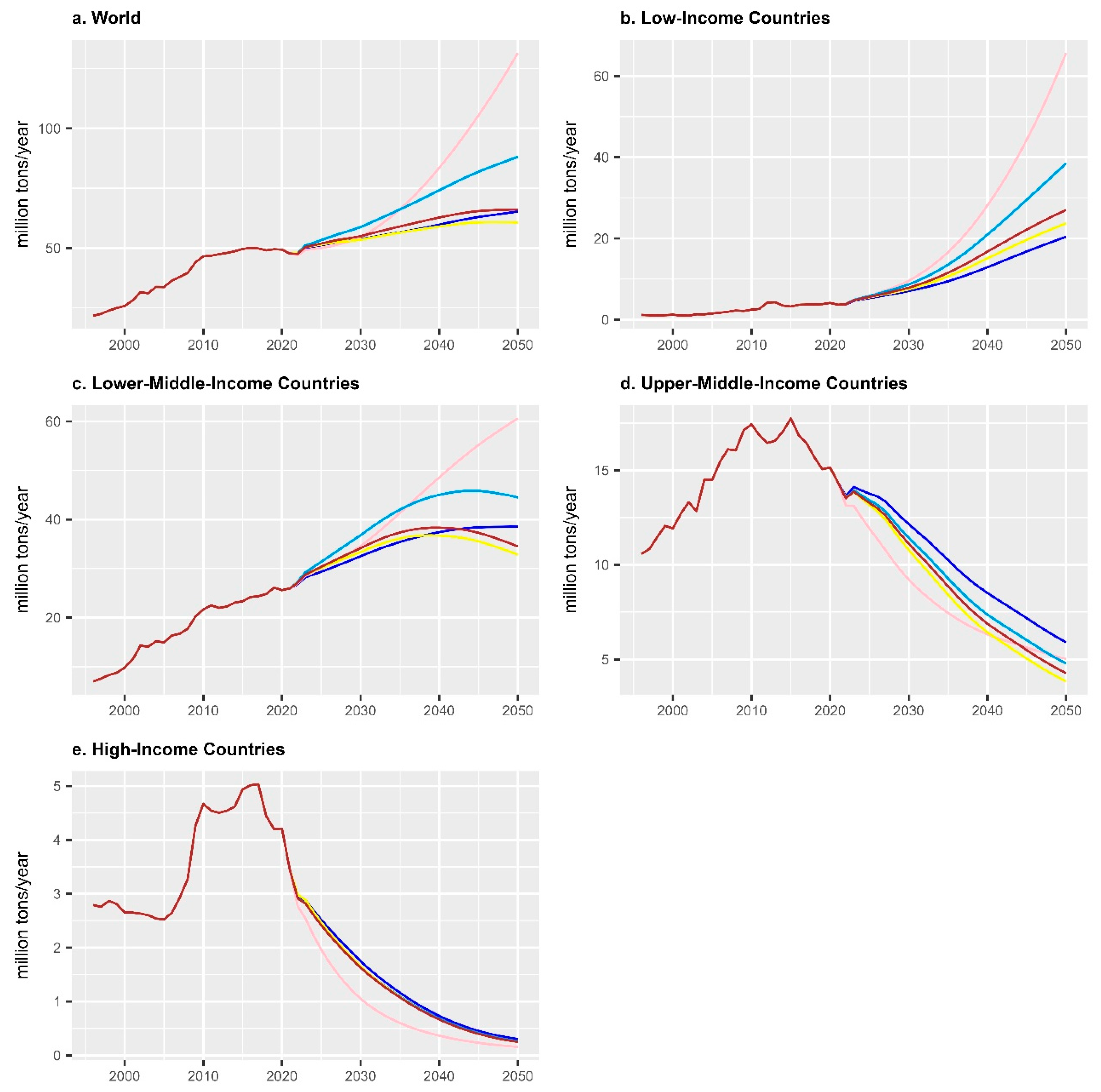
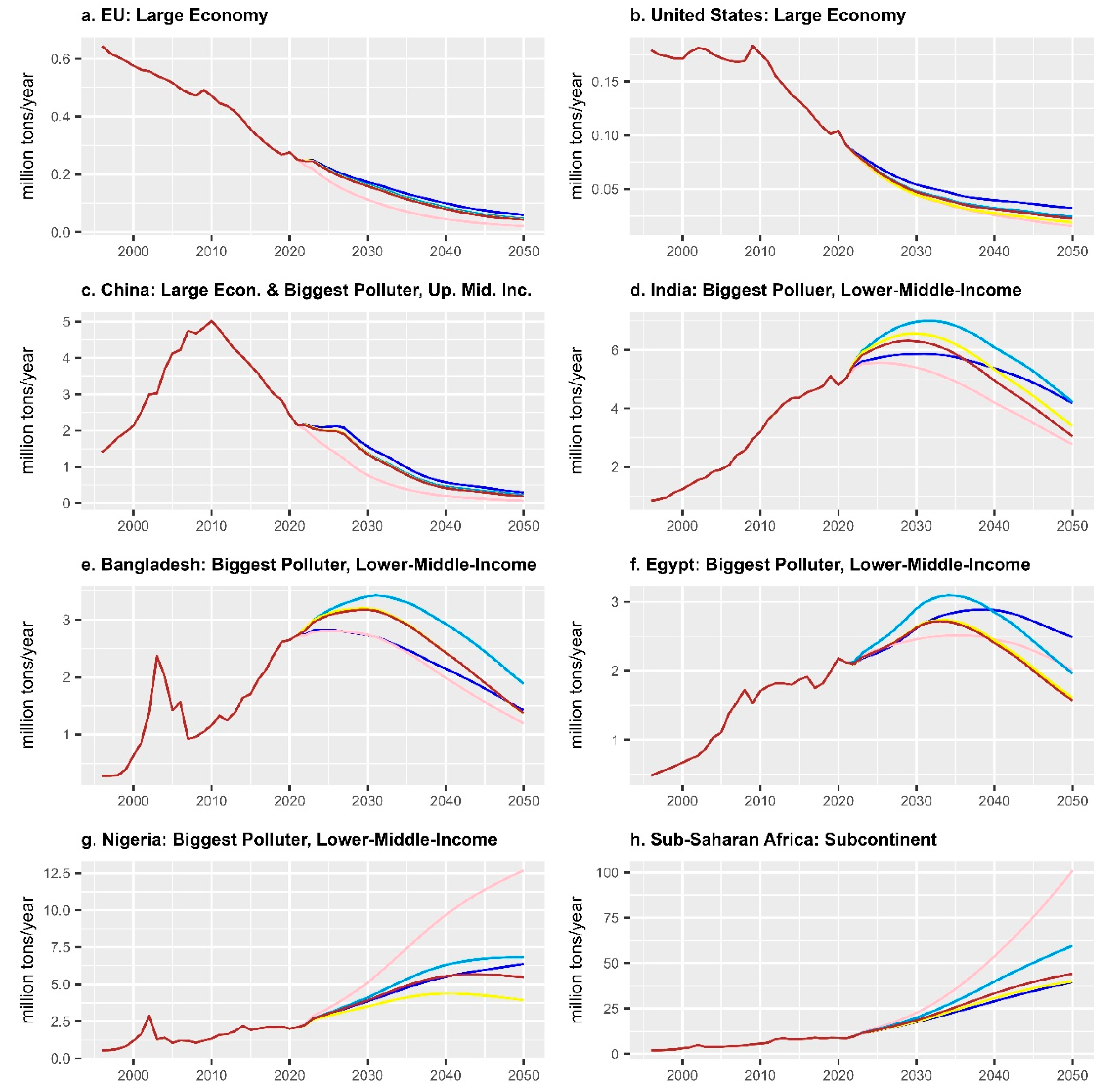
The impact of changes in population structure, urbanization, and urban primacy had not been studied in the scenario analysis of global plastic pollution. These scenarios analyzed the differences based on GDP, population structure, URB, and UPRI. They demonstrated the sensitivity of the projections to the changes in assumptions. For Scenarios A–D, except for the specific variables mentioned (e.g., GDP per capita), all other variables changed according to the BAU scenario. In scenario analyses, the data recently updated by the World Bank were used rather than those used in model estimates. Although some data used for model estimation and scenarios were not identical, all the results presented in this study are replicable and verifiable.

3.2.2. Projections

Figure 1 and Figure 2 show the key projections of the annual plastic pollutant emissions. Figure 1 shows the global population and groups by income level. The income level is crucial in this model because it determines the EKC relationship. Figure 2 includes large economies, the largest polluters, and regions, providing further implications for global plastic pollution.

Global Scale

The BAU scenario estimated that the global annual emissions of plastic pollution reached 50.5 MT/y in 2023 and would reach 66.1 MT/y by 2050 (Figure 1a). Plastic pollution may continue to increase from 2022 to 2050 but more slowly than that from 1996 to 2015. This result is consistent with those obtained using other global models published recently with low estimates [3,11,14,63]. Cordier et al. [14] and Lau et al. [3] estimated the BAU scenario to produce plastic pollution between 61.2 and 110.2 MT/y by 2050 and 71.9 and 147.6 MT/y by 2040 (no simulation had been performed beyond 2040), respectively; however, our projection was 62.8 MT/y by 2040. According to Lebreton and Andrady [63], the low, mid, and high estimates of plastic pollution by 2050 were 137.3, 187.1, and 226.2 MT/y, respectively. An OECD study projected plastic pollution to be 131.9 MT/y by 2050 [11].

Some differences existed between previous approaches, and these led to different projections. For example, Cordier et al. [14] adopted econometric models, including the EKC relationship, as in this study; however, they were built on a cross-sectional dataset rather than on a panel dataset. The current model can be considered reliable because it accounted for evolution over time. Cordier et al. [14] applied each model to a set of three statistical equations that were multiplied to estimate the inadequately managed plastic waste but did not consider the interactions between the explanatory variables from those three equations. Furthermore, they focused on corruption and lack of education, whereas these models were built on the STIRPAT framework, which is more comprehensive. The study by Lau et al. [3] differs from the current study in the following ways. First, they designed their model based on municipal solid waste data for each country provided by the World Bank (2018) [44]; however, the World Bank (2012) [45] database was included in the design of the STIRPAT model in our study to enrich the dataset and apply it to a panel data model. Second, they assumed that per capita waste generation increased with per capita income and stabilized at 120 kg/y at a per capita income level of USD 40,000; however, our model included the EKC relationship. Third, the factors were comprehensively included in our study based on the STIRPAT framework, which was lacking in the study by Lau et al. [3]. Fourth, they included primary microplastic emissions in their estimations, whereas only macroplastics emissions were included in the current study. Finally, similar to Lebreton and Andrady [63], the authors [3] included individual littering (plastic waste directly dumped into waterways and coastal waters by residents), unlike our study, and this may have led us to the underestimation of plastic pollution. Although Lebreton and Andrady [63] used factors that are similar to those in this STIRPAT model (GDP per capita, population size, and urban vs. rural areas), they used a different database to design their model [68]. Furthermore, rather than applying the EKC relationship using the squared term of GDPPC, as in this model, Lebreton and Andrady [63] included a negative correlation between GDPPC and the fraction of unsound disposal.

These scenarios produced unexpected projections. Scenarios B and C projected more plastic pollution in 2050 (131.5 MT and 88.1 MT, respectively) than BAU; however, Scenarios A and D projected less plastic pollution (65.3 MT and 60.7 MT, respectively) than BAU. A high pollution level was expected, but a low level was not, owing to the signs of the coefficients in the model (model specification (6) RE in Table 2). The impact of slow GDP per capita growth (Scenario A) was subtle compared to that of the BAU scenario. Although Scenario D was expected to lead to more plastic pollution, it was less than that of BAU. This is because each country was influenced by the scenarios to different degrees and even in opposite directions. Therefore, the total global value (that is, an aggregate of the plastic pollution from heterogeneous countries) could be more or less than that in the BAU, depending on the heterogeneities. This necessitates an investigation of heterogeneity by country and certain groups, such as income groups, to elucidate policy implications.

Income Level

Global trends in plastic pollution can be explained by heterogeneities in income level. These trends varied by income level and followed the EKC relationship (Figure 1b–e). Low-income countries experienced increased plastic pollution under any scenario (Figure 1b). Lower-middle-income countries showed mixed projections, with a decline in some countries under all scenarios but continued to increase under Scenario B (Figure 1c). Upper-middle- and high-income countries have already started reducing plastic pollution around 2010–2015 (Figure 1d,e). However, the reduction in these countries is outweighed by the increase in plastic pollution from low- and lower-middle-income countries. Scenario B exhibited the most extreme differences, resulting in a significant global increase in plastic pollution. In high- and upper-middle-income countries, a decrease in the 15–64 age group reduced plastic pollution. In contrast, in low- and lower-middle-income countries, an increase in the same age group results in increased plastic pollution. Globally, the plastic pollution in developing countries outweighs the decrease in developed countries, and this will lead to a sharp increase in plastic pollution by 2050.

Key Countries

The identification of the key polluting countries provided further insights into the level of plastic pollution. Figure 2 highlights three large economies (the European Union [EU], the United States of America [USA], and China); the top five polluters as of 2021 (China, India, Bangladesh, Egypt, and Nigeria); and one subcontinent (sub-Saharan Africa). The top five polluters accounted for 30% of the total plastic pollution. Although the three large economies differed in their past trends, all were projected to significantly reduce plastic pollutant emissions and approach zero. EU countries have reduced plastic pollution since a quarter of a century ago, whereas the USA began to reduce plastic pollution approximately 15 years ago. China, which was a major polluter as of 2021, has started to reduce plastic pollution along with the USA. These differ from the projection by the OECD [11] that a decline in the proportion of mismanaged plastic waste and an increase in its absolute amount will occur by 2050. The other largest polluters, except for Nigeria, are expected to decrease their pollution levels before 2050. However, the reduction was below the level reached by Egypt in 2021 under Scenario A. Notably, the order of the scenarios of the countries for pollution in 2050 varied even when the countries followed a similar pattern of reaching a peak in the future (as projected by the EKC relationship). For example, regarding 2050 pollution levels, Scenario C was the worst for India and Bangladesh, whereas Scenario A was the worst for Egypt. This difference suggests that factors other than the EKC relationship influence the pollution dynamics. Overall, pollution will continue to increase in Nigeria, the fifth-largest polluter as of 2021. In particular, pollution in Nigeria could increase from 2.10 MT in 2021 to 12.69 MT in 2050 under Scenario B because of the rapid growth of the 15–64 age group. Nigeria is on the sub-Saharan continent (Figure 2h), with similar or more aggravating patterns (i.e., monotonically increasing pollution under any scenario). It is the only subcontinent that showed monotonic increases in the future under any scenario (figures by subcontinent can be created using the PivotTable provided in the Supplementary Materials). Therefore, the sub-Saharan continent is a major region contributing to the future increase in global plastic pollution.

4. Discussion

The scenario analyses of the STIRPAT model applied in this study revealed the impact of socioeconomic driving forces on future projections of plastic pollution on a national and global scale. This facilitated the identification of the target locations and factors for the effective prevention of future plastic pollution. Consequently, four policy implications were proposed. First, low- and lower-middle-income countries, particularly sub-Saharan Africa, must be targeted because, following the EKC relationship, they may become the main contributors to plastic pollution, accounting for 66.8% of the world total under BAU by 2050. Plastic pollutants emitted by high-income countries will be nearly zero in any scenario by 2050. Accordingly, these countries can achieve the Osaka Blue Ocean Vision shared in the G20 Summit, which aims to achieve zero additional plastic waste emissions into the ocean by 2050 [69]. However, this does not imply that high-income countries should not prevent plastic pollution, because the target value of zero indicates the emission flow per year and not the total stock of plastic pollution that accumulates in the environment [70], and flow is determined by the speed of accumulation. A previous study reported that the weight of marine plastic waste will exceed that of fish by 2050 [71]. Therefore, all countries, including high-income countries, should make more urgent efforts to remove plastics from their environment before they degrade into microplastics, which are even more difficult to remove. Furthermore, this model did not consider the impact of the plastic waste trade, mostly from higher- to lower-income countries [72,73], and only exporters are expected to manage plastic waste; thus, further studies on this aspect will provide more accurate projections of plastic pollution (e.g., OECD [11]).

Second, Scenario B (change in population structure) was expected to result in more plastic pollution than BAU, because of the importance of targeting the increasing working-age population (15–64 age group), especially in low-income, lower-middle-income, and sub-Saharan countries (Figure 1b,c and Figure 2h). Policymakers should formulate appropriate policies to change the behavior of these polluting countries. A combination of regulatory, market-based, and behavioral instruments may be required to induce suitable behavioral changes [74]. Regulation of the consumer market with, for example, bans on single-use plastic products is a powerful tool in many countries [74,75]. The recent literature emphasized that behavioral instruments should complement regulatory policies and market-based measures to produce long-lasting effects on pollutant-emitting behavior [74,76]. Therefore, government interventions should involve milder informative instruments, such as awareness campaigns, education programs, and recommended guidelines. Nonetheless, the effectiveness of these measures may be context-dependent, and effective measures in one region may not be the same in another [77,78]. For example, measures commonly used in Europe may not work for the targeted low-income, lower-to-middle-income, and sub-Saharan countries. Informative measures used in Europe [79] may not be effective in the targeted countries owing to the pre-existing interest of people in environmental issues and their willingness to engage in pro-environmental behaviors [80]. As suggested by the EKC relationship, the interest of people in environmental issues in such countries may be limited. Although the main targets are low- and lower-middle-income countries, high-income countries may play a crucial role in technological transfer [81]. The mobilization of large-scale monumental innovations can play a significant role in achieving a circular economy with sustainable plastic use [63]. In other words, innovations and their transfer to low- and lower-middle-income countries could help maintain steady economic growth and minimize plastic pollution.

Third, Scenario C (rapid urbanization) could reduce future increases in plastic pollution, especially in low-income and sub-Saharan countries (Figure 1b,c and Figure 2h). The inextricable link between urbanization and plastic waste management increases the urgency to develop effective policy responses to address this challenge [82]. That is, urban planners should integrate plastic waste management into urban development strategies by following circular economic principles. A circular economic approach aims to reduce the use of raw materials, reuse already processed materials, and recycle waste [83]. As part of a circular economy, plastic waste management requires highly integrated perspectives throughout the life cycle of plastics, from production to consumption to waste and pollution [84]. Urban spatial planning facilitates circular action by relocating the producers and consumers of plastic waste to urban areas. Accordingly, infrastructure delivery is crucial for the socioecological transformation of urban systems [85,86,87]. For instance, China has strongly promoted the construction of a new type of urbanization that requires layout optimization of urban spatial structures [88]. As previously discussed for Scenario B, high-income countries could play a significant role in helping low-income and sub-Saharan countries tackle urbanization.

Finally, although the estimations could reveal whether the pollution level in a country is increasing or declining in accordance with the EKC relationship, policymakers should not adopt a passive attitude toward plastic pollution control. Therefore, policymakers must design sustainable, growth-oriented policies and strategies to reduce plastic pollution. As previously discussed, the stoppage of annual plastic pollution does not imply the removal of accumulated plastics since the 1950s.

5. Conclusions

This study developed a STIRPAT model to conduct scenario analyses and investigate the impacts of sociodemographic driving forces on future plastic pollution by 2050 on a national (217 countries) and global scale. The empirical findings confirmed the EKC relationship and demonstrated that population structure and urbanization changes could substantially affect plastic pollution. Scenario analyses identified the heterogeneity of impacts according to country, income, and subcontinent levels. For example, high-income and upper-middle-income countries will significantly reduce plastic pollution, whereas low-income countries and sub-Saharan Africa are projected to become major contributors to plastic pollution, leading to a global trend of increasing plastic pollution. Therefore, understanding these heterogeneities will help policymakers identify targets to effectively reduce future global plastic pollution.

This study has some limitations and recommendations for policymakers and future research. First, data availability was a major limitation of the model; therefore, future research should include additional data panels to provide more reliable estimates. Second, the findings serve as a basis for advancing our knowledge on the impacts of urbanization; thus, future investigations should include rural–urban migration, mixed land use, and monocentric/polycentric urban forms to reveal more detailed information on the effects of urbanization on plastic pollution. Third, future studies should explore the spillover effects of plastic regulation policies in developing countries. For example, China imposed a ban on the import of plastic waste in 2017, leading to a change in the structure of the international plastic waste trade, thereby making an additional impact on the distribution of plastic waste pollution [63]. Fourth, this study did not intend to identify an absolute law but shed more light on the EKC relationship using the STIRPAT model. Therefore, further studies that consider more factors and involve collaborative effort among stakeholders are needed. Finally, utilizing recently developed spatiotemporal data to trace plastic footprints can further refine the policy implications proposed by this study. For example, the National Aeronautics and Space Administration (NASA) developed a system that can spatiotemporally detect marine microplastic concentrations [89].

References

1. Barnes, S.J. Understanding plastics pollution: The role of economic development and technological research. Environ. Pollut. 2019, 249, 812–821. [Google Scholar] [CrossRef] [PubMed]
2. Issifu, I.; Sumaila, U.R. A review of the production, recycling and management of marine plastic pollution. J. Mar. Sci. Eng. 2020, 8, 945. [Google Scholar] [CrossRef]
3. Lau, W.W.Y.; Shiran, Y.; Bailey, R.M.; Cook, E.; Stuchtey, M.R.; Koskella, J.; Velis, C.A.; Godfrey, L.; Boucher, J.; Murphy, M.B.; et al. Evaluating scenarios toward zero plastic pollution. Science 2020, 369, 1455–1461. [Google Scholar] [CrossRef] [PubMed]
4. Geyer, R.; Jambeck, J.R.; Law, K.L. Production, use, and fate of all plastics ever made. Sci. Adv. 2017, 3, e1700782. [Google Scholar] [CrossRef]
5. WWF-Australia. The Lifecycle of Plastics. Available online: https://wwf.org.au/blogs/the-lifecycle-of-plastics (accessed on 26 December 2023).
6. OECD. Global Plastics Outlook: Economic Drivers, Environmental Impacts and Policy Options; OECD Publishing: Paris, France, 2022. [Google Scholar]
7. Cordier, M.; Uehara, T. How much innovation is needed to protect the ocean from plastic contamination? Sci. Total Environ. 2019, 670, 789–799. [Google Scholar] [CrossRef]
8. GESAMP. Sources, fate and effects of microplastics in the marine environment: A global assessment. In GESAMP Reports and Studies; Kershaw, P.J., Ed.; IMO Publishing: London, UK, 2015. [Google Scholar]
9. Villarrubia-Gómez, P.; Cornell, S.E.; Fabres, J. Marine plastic pollution as a planetary boundary threat—The drifting piece in the sustainability puzzle. Mar. Policy 2018, 96, 213–220. [Google Scholar] [CrossRef]
10. Woods, J.S.; Verones, F.; Jolliet, O.; Vázquez-Rowe, I.; Boulay, A.-M. A framework for the assessment of marine litter impacts in life cycle impact assessment. Ecol. Indic. 2021, 129, 107918. [Google Scholar] [CrossRef]
11. OECD. Global Plastics Outlook: Policy Scenarios to 2060; OECD Publishing: Paris, France, 2022. [Google Scholar]
12. Lau, L.-S.; Yii, K.-J.; Ng, C.-F.; Tan, Y.-L.; Yiew, T.-H. Environmental Kuznets curve (EKC) hypothesis: A bibliometric review of the last three decades. Energy Environ. 2023, 0958305X231177734. [Google Scholar] [CrossRef]
13. Chen, D.M.-C.; Bodirsky, B.L.; Krueger, T.; Mishra, A.; Popp, A. The world’s growing municipal solid waste: Trends and impacts. Environ. Res. Lett. 2020, 15, 074021. [Google Scholar] [CrossRef]
14. Cordier, M.; Uehara, T.; Baztan, J.; Jorgensen, B.; Yan, H. Plastic pollution and economic growth: The influence of corruption and lack of education. Ecol. Econ. 2021, 182, 106930. [Google Scholar] [CrossRef]
15. Dietz, T.; Rosa, E.A. Effects of population and affluence on CO2 emissions. Proc. Natl. Acad. Sci. USA 1997, 94, 175–179. [Google Scholar] [CrossRef]
16. Wei, T. What STIRPAT tells about effects of population and affluence on the environment? Ecol. Econ. 2011, 72, 70–74. [Google Scholar] [CrossRef]
17. York, R.; Rosa, E.A.; Dietz, T. STIRPAT, IPAT and ImPACT: Analytic tools for unpacking the driving forces of environmental impacts. Ecol. Econ. 2003, 46, 351–365. [Google Scholar] [CrossRef]
18. Liu, Y.; Han, Y. Impacts of urbanization and technology on carbon dioxide emissions of Yangtze River economic Belt at two stages: Based on an extended STIRPAT model. Sustainability 2021, 13, 7022. [Google Scholar] [CrossRef]
19. Martínez-Zarzoso, I.; Maruotti, A. The impact of urbanization on CO2 emissions: Evidence from developing countries. Ecol. Econ. 2011, 70, 1344–1353. [Google Scholar] [CrossRef]
20. Poumanyvong, P.; Kaneko, S. Does urbanization lead to less energy use and lower CO2 emissions? A cross-country analysis. Ecol. Econ. 2010, 70, 434–444. [Google Scholar] [CrossRef]
21. Ehigiamusoe, K.U.; Lean, H.H.; Somasundram, S. Unveiling the non-linear impact of sectoral output on environmental pollution in Malaysia. Environ. Sci. Pollut. Res. Int. 2022, 29, 7465–7488. [Google Scholar] [CrossRef]
22. Jia, J.; Deng, H.; Duan, J.; Zhao, J. Analysis of the major drivers of the ecological footprint using the STIRPAT model and the PLS method—A case study in Henan Province, China. Ecol. Econ. 2009, 68, 2818–2824. [Google Scholar] [CrossRef]
23. Xu, C.; Zhao, W.; Zhang, M.; Cheng, B. Pollution haven or halo? The role of the energy transition in the impact of FDI on SO2 emissions. Sci. Total Environ. 2021, 763, 143002. [Google Scholar] [CrossRef]
24. Yang, R.; Chen, W. Spatial correlation, influencing factors and environmental supervision on mechanism construction of atmospheric pollution: An empirical study on SO2 emissions in China. Sustainability 2019, 11, 1742. [Google Scholar] [CrossRef]
25. Dong, Q.; Lin, Y.; Huang, J.; Chen, Z. Has urbanization accelerated PM2.5 emissions? An empirical analysis with cross-country data. China Econ. Rev. 2020, 59, 101381. [Google Scholar] [CrossRef]
26. Ji, X.; Yao, Y.; Long, X. What causes PM2.5 pollution? Cross-economy empirical analysis from socioeconomic perspective. Energy Policy 2018, 119, 458–472. [Google Scholar] [CrossRef]
27. Zhang, Y.; Sun, M.; Yang, R.; Li, X.; Zhang, L.; Li, M. Decoupling water environment pressures from economic growth in the Yangtze River Economic Belt, China. Ecol. Indic. 2021, 122, 107314. [Google Scholar] [CrossRef]
28. Charles-Edwards, E.; Wilson, T.; Bernard, A.; Wohland, P. How will COVID-19 impact Australia’s future population? A scenario approach. Appl. Geogr. 2021, 134, 102506. [Google Scholar] [CrossRef]
29. Cole, M.A.; Neumayer, E. Examining the impact of demographic factors on air pollution. Popul. Environ. 2004, 26, 5–21. [Google Scholar] [CrossRef]
30. Goel, R.K.; Herrala, R.; Mazhar, U. Institutional quality and environmental pollution: MENA countries versus the rest of the world. Econ. Syst. 2013, 37, 508–521. [Google Scholar] [CrossRef]
31. Li, K.; Fang, L.; He, L. How population and energy price affect China’s environmental pollution? Energy Policy 2019, 129, 386–396. [Google Scholar] [CrossRef]
32. Qin, B.; Wu, J. Does urban concentration mitigate CO2 emissions? Evidence from China 1998–2008. China Econ. Rev. 2015, 35, 220–231. [Google Scholar] [CrossRef]
33. Zhang, N.; Yu, K.; Chen, Z. How does urbanization affect carbon dioxide emissions? A cross-country panel data analysis. Energy Policy 2017, 107, 678–687. [Google Scholar] [CrossRef]
34. Wooldridge, J.M. Econometric Analysis of Cross Section and Panel Data; MIT Press: London, UK, 2010. [Google Scholar]
35. Feng, K.; Hubacek, K.; Guan, D. Lifestyles, technology and CO2 emissions in China: A regional comparative analysis. Ecol. Econ. 2009, 69, 145–154. [Google Scholar] [CrossRef]
36. Shafiei, S.; Salim, R.A. Non-renewable and renewable energy consumption and CO2 emissions in OECD countries: A comparative analysis. Energy Policy 2014, 66, 547–556. [Google Scholar] [CrossRef]
37. Hua, Y.; Xie, R.; Su, Y. Fiscal spending and air pollution in Chinese cities: Identifying composition and technique effects. China Econ. Rev. 2018, 47, 156–169. [Google Scholar] [CrossRef]
38. Salim, R.; Rafiq, S.; Shafiei, S.; Yao, Y. Does urbanization increase pollutant emission and energy intensity? Evidence from some Asian developing economies. Appl. Econ. 2019, 51, 4008–4024. [Google Scholar] [CrossRef]
39. Wang, Y.; Liao, M.; Wang, Y.; Xu, L.; Malik, A. The impact of foreign direct investment on China’s carbon emissions through energy intensity and emissions trading system. Energy Econ. 2021, 97, 105212. [Google Scholar] [CrossRef]
40. Pham, N.M.; Huynh, T.L.D.; Nasir, M.A. Environmental consequences of population, affluence and technological progress for European countries: A Malthusian view. J. Environ. Manag. 2020, 260, 110143. [Google Scholar] [CrossRef] [PubMed]
41. Xu, F.; Huang, Q.; Yue, H.; He, C.; Wang, C.; Zhang, H. Reexamining the relationship between urbanization and pollutant emissions in China based on the STIRPAT model. J. Environ. Manag. 2020, 273, 111134. [Google Scholar] [CrossRef] [PubMed]
42. Shi, A. The impact of population pressure on global carbon dioxide emissions, 1975–1996: Evidence from pooled cross-country data. Ecol. Econ. 2003, 44, 29–42. [Google Scholar] [CrossRef]
43. Leitão, A. Corruption and the environmental Kuznets curve: Empirical evidence for sulfur. Ecol. Econ. 2010, 69, 2191–2201. [Google Scholar] [CrossRef]
44. World Bank Group; Kaza, S.; Yao, L.; Bhada-Tata, P.; Van Woerden, F. What a Waste 2.0: A Global Snapshot of Solid Waste Management to 2050; World Bank Publications: Washington, DC, USA, 2018; Available online: https://openknowledge.worldbank.org/handle/10986/30317 (accessed on 4 November 2023).
45. World Bank Group; Hoornweg, D.; Bhada-Tata, P. What a Waste: A Global Review of Solid Waste Management; World Bank Publications: Washington, DC, USA, 2012; Available online: https://openknowledge.worldbank.org/handle/10986/17388 (accessed on 4 November 2023).
46. World Bank DataBank. World Governance Indicators. 2023. Available online: https://databank.worldbank.org/source/worldwide-governance-indicators (accessed on 4 November 2023).
47. Field, A.; Miles, J.; Field, Z. Discovering Statistics Using R; SAGE Publications Ltd.: London, UK, 2012. [Google Scholar]
48. Myers, R.H. Classical and Modern Regression with Applications, 2nd ed.; Thompson Publishing Learning: Boston, MA, USA, 1990. [Google Scholar]
49. Baltagi, H.B. Econometric Analysis of Panel Data, 3rd ed.; John Wiley & Sons, Ltd.: Chichester, UK, 2005. [Google Scholar]
50. Kimino, S.; Saal, D.S.; Driffield, N. Macro determinants of FDI inflows to Japan: An analysis of source country characteristics. World Econ. 2007, 30, 446–469. [Google Scholar] [CrossRef]
51. Park, S.; Lee, Y. Regional model of EKC for air pollution: Evidence from the Republic of Korea. Energy Policy 2011, 39, 5840–5849. [Google Scholar] [CrossRef]
52. Dinda, S. Environmental Kuznets curve hypothesis: A survey. Ecol. Econ. 2004, 49, 431–455. [Google Scholar] [CrossRef]
53. Roca, J.; Padilla, E.; Farré, M.; Galletto, V. Economic growth and atmospheric pollution in Spain: Discussing the environmental Kuznets curve hypothesis. Ecol. Econ. 2001, 39, 85–99. [Google Scholar] [CrossRef]
54. Sulemana, I.; James, H.S.; Rikoon, J.S. Environmental Kuznets Curves for air pollution in African and developed countries: Exploring turning point incomes and the role of democracy. J. Environ. Econ. Policy 2017, 6, 134–152. [Google Scholar] [CrossRef]
55. Awaworyi Churchill, S.A.; Inekwe, J.; Ivanovski, K.; Smyth, R. The environmental Kuznets curve across Australian states and territories. Energy Econ. 2020, 90, 104869. [Google Scholar] [CrossRef]
56. Dikareva, N.; Simon, K.S. Microplastic pollution in streams spanning an urbanisation gradient. Environ. Pollut. 2019, 250, 292–299. [Google Scholar] [CrossRef]
57. Liddle, B. Consumption-driven environmental impact and age structure change in OECD countries: A cointegration-STIRPAT analysis. DemRes 2011, 24, 749–770. [Google Scholar] [CrossRef]
58. Gifford, R.; Nilsson, A. Personal and social factors that influence pro-environmental concern and behaviour: A review. Int. J. Psychol. 2014, 49, 141–157. [Google Scholar] [CrossRef]
59. Hartley, B.L.; Pahl, S.; Veiga, J.; Vlachogianni, T.; Vasconcelos, L.; Maes, T.; Doyle, T.; d’Arcy Metcalfe, R.D.A.; Öztürk, A.A.; Di Berardo, M.; et al. Exploring public views on marine litter in Europe: Perceived causes, consequences and pathways to change. Mar. Pollut. Bull. 2018, 133, 945–955. [Google Scholar] [CrossRef]
60. IPCC; Nakicenovic, N.; Swart, R. (Eds.) The Edinburgh Building Shaftesbury Road, Cambridge; Cambridge University Press: Cambridge, UK, 2000; p. 570. Available online: https://www.ipcc.ch/report/emissions-scenarios (accessed on 4 November 2023).
61. Jambeck, J.R.; Geyer, R.; Wilcox, C.; Siegler, T.R.; Perryman, M.; Andrady, A.; Narayan, R.; Law, K.L. Marine pollution. Plastic waste inputs from land into the ocean. Science 2015, 347, 768–771. [Google Scholar] [CrossRef]
62. Koelmans, A.A.; Kooi, M.; Law, K.L.; Van Sebille, E. All is not lost: Deriving a top-down mass budget of plastic at sea. Environ. Res. Lett. 2017, 12, 114028. [Google Scholar] [CrossRef]
63. Lebreton, L.; Andrady, A. Future scenarios of global plastic waste generation and disposal. Palgrave Commun. 2019, 5, 6. [Google Scholar] [CrossRef]
64. Borrelle, S.B.; Ringma, J.; Law, K.L.; Monnahan, C.C.; Lebreton, L.; McGivern, A.; Murphy, E.; Jambeck, J.; Leonard, G.H.; Hilleary, M.A.; et al. Predicted growth in plastic waste exceeds efforts to mitigate plastic pollution. Science 2020, 369, 1515–1518. [Google Scholar] [CrossRef] [PubMed]
65. Peng, Y.; Wu, P.; Schartup, A.T.; Zhang, Y. Plastic waste release caused by COVID-19 and its fate in the global ocean. Proc. Natl. Acad. Sci. USA 2021, 118, e2111530118. [Google Scholar] [CrossRef]
66. Fan, Y.V.; Jiang, P.; Tan, R.R.; Aviso, K.B.; You, F.; Zhao, X.; Lee, C.T.; Klemeš, J.J. Forecasting plastic waste generation and interventions for environmental hazard mitigation. J. Hazard. Mater. 2022, 424, 127330. [Google Scholar] [CrossRef]
67. Peterson, G.D.; Cumming, G.S.; Carpenter, S.R. Scenario planning: A tool for conservation in an uncertain world. Conserv. Biol. 2003, 17, 358–366. [Google Scholar] [CrossRef]
68. D-Waste. Waste Atlas. 2016. Available online: http://www.atlas.d-waste.com (accessed on 4 November 2023).
69. Ministry of the Environment Japan. G20 Report on Actions against Marine Plastic Litter: Third Information Sharing Based on the G20 Implementation Framework 2021, 2nd ed.; Ministry of the Environment: Tokyo, Japan, 2021. Available online: https://www.env.go.jp/press/files/en/938.pdf (accessed on 4 November 2023).
70. Uehara, T. Can young generations recognize marine plastic waste as a systemic issue? Sustainability 2020, 12, 2586. [Google Scholar] [CrossRef]
71. World Economic Forum, Ellen MacArthur Foundation and McKinsey & Company, The New Plastics Economy—Rethinking the future of plastics. 2016. Available online: https://www.ellenmacarthurfoundation.org/the-new-plastics-economy-rethinking-the-future-of-plastics (accessed on 4 November 2023).
72. Liang, Y.; Tan, Q.; Song, Q.; Li, J. An analysis of the plastic waste trade and management in Asia. Waste Manag. 2021, 119, 242–253. [Google Scholar] [CrossRef]
73. Wang, C.; Zhao, L.; Lim, M.K.; Chen, W.-Q.; Sutherland, J.W. Structure of the global plastic waste trade network and the impact of China’s import Ban. Resour. Conserv. Recycl. 2020, 153, 104591. [Google Scholar] [CrossRef]
74. Alpizar, F.; Carlsson, F.; Lanza, G.; Carney, B.; Daniels, R.C.; Jaime, M.; Ho, T.; Nie, Z.; Salazar, C.; Tibesigwa, B.; et al. A framework for selecting and designing policies to reduce marine plastic pollution in developing countries. Environ. Sci. Policy 2020, 109, 25–35. [Google Scholar] [CrossRef]
75. Fadeeva, Z.; Van Berkel, R. Unlocking circular economy for prevention of marine plastic pollution: An exploration of G20 policy and initiatives. J. Environ. Manag. 2021, 277, 111457. [Google Scholar] [CrossRef]
76. Kirakozian, A. One without the other? Behavioural and incentive policies for household waste management. J. Econ. Surv. 2016, 30, 526–551. [Google Scholar] [CrossRef]
77. Uehara, T.; Asari, M.; Sakurai, R. Knowing the rules can effectively enhance plastic waste separation on campus. Front. Sustain. 2022, 3, 1023605. [Google Scholar] [CrossRef]
78. Uehara, T.; Asari, M.; Sakurai, R.; Cordier, M.; Kalyanasundaram, M. Behavioral barrier-based framework for selecting intervention measures toward sustainable plastic use and disposal. J. Clean. Prod. 2023, 384, 135609. [Google Scholar] [CrossRef]
79. European Environment Agency. Preventing Plastic Waste in Europe; Publications Office of the European Union: Luxembourg, 2019; Available online: https://www.eea.europa.eu/publications/preventing-plastic-waste-in-europe/at_download/file (accessed on 4 November 2023).
80. Grilli, G.; Curtis, J. Encouraging pro-environmental behaviours: A review of methods and approaches. Renew. Sustain. Energy Rev. 2021, 135, 110039. [Google Scholar] [CrossRef]
81. De Mello, L.R. Foreign direct investment in developing countries and growth: A selective survey. J. Dev. Stud. 1997, 34, 1–34. [Google Scholar] [CrossRef]
82. Bari, Q.H.; Mahbub Hassan, K.M.; Haque, R. Scenario of solid waste reuse in Khulna city of Bangladesh. Waste Manag. 2012, 32, 2526–2534. [Google Scholar] [CrossRef] [PubMed]
83. Burneo, D.; Cansino, J.M.; Yñiguez, R. Environmental and socioeconomic impacts of urban waste recycling as part of circular economy. The case of Cuenca (Ecuador). Sustainability 2020, 12, 3406. [Google Scholar] [CrossRef]
84. Nielsen, T.D.; Hasselbalch, J.; Holmberg, K.; Stripple, J. Politics and the plastic crisis: A review throughout the plastic life cycle. WIREs Energy Environ. 2020, 9, e360. [Google Scholar] [CrossRef]
85. Bolger, K.; Doyon, A. Circular cities: Exploring local government strategies to facilitate a circular economy. Eur. Plan. Stud. 2019, 27, 2184–2205. [Google Scholar] [CrossRef]
86. Savini, F. The economy that runs on waste: Accumulation in the circular city. J. Environ. Policy Plan. 2019, 21, 675–691. [Google Scholar] [CrossRef]
87. Williams, J. The role of spatial planning in transitioning to circular urban development. Urban Geogr. 2020, 41, 915–919. [Google Scholar] [CrossRef]
88. Lin, B.; Zhu, J. Impact of China’s new-type urbanization on energy intensity: A city-level analysis. Energy Econ. 2021, 99, 105292. [Google Scholar] [CrossRef]
89. Evans, M.C.; Ruf, C.S. Toward the detection and imaging of ocean microplastics with a spaceborne radar. IEEE Trans. Geosci. Remote Sens. 2022, 60, 4202709. [Google Scholar] [CrossRef]
90. Dunlap, R.E.; Mertig, A.G. Global concern for the environment: Is affluence a prerequisite? J. Soc. Issues 1995, 51, 121–137. [Google Scholar] [CrossRef]
91. Stern, D.I. The rise and fall of the environmental Kuznets curve. World Dev. 2004, 32, 1419–1439. [Google Scholar] [CrossRef]
92. D’Amato, A.; Mazzanti, M.; Nicolli, F.; Zoli, M. Illegal waste disposal: Enforcement actions and decentralized environmental policy. Socio-Econ. Plan. Sci. 2018, 64, 56–65. [Google Scholar] [CrossRef]
93. Santos, A.C.; Mendes, P.; Teixeira, M.R. Social life cycle analysis as a tool for sustainable management of illegal waste dumping in municipal services. J. Clean. Prod. 2019, 210, 1141–1149. [Google Scholar] [CrossRef]
94. Tisserant, A.; Pauliuk, S.; Merciai, S.; Schmidt, J.; Fry, J.; Wood, R.; Tukker, A. Solid waste and the circular economy: A global analysis of waste treatment and waste footprints. J. Ind. Ecol. 2017, 21, 628–640. [Google Scholar] [CrossRef]
Figure 1. Projections of plastic pollution worldwide based on income levels of the countries. Brown: BAU (business-as-usual), blue: Scenario A (slow GDP), pink: Scenario B (change in population structure), light blue: Scenario C (urbanization), and yellow: Scenario D (urban primacy).
Sustainability 16 00643 g001
Figure 2. Projections of plastic pollution for large economies, biggest polluters, and a subcontinent region. Brown: BAU (business-as-usual), blue: Scenario A (slow GDP), pink: Scenario B (change in population structure), light blue: Scenario C (urbanization), and yellow: Scenario D (urban primacy). Econ.: economy, Up. Mid. Inc.: Upper-middle-income.
Sustainability 16 00643 g002