Optimization of State of the Art Fuzzy-Based Machine Learning Techniques for Total Dissolved Solids Prediction

Abstract

Total dissolved solid prediction is an important factor which can support the early warning of water pollution, especially in the areas exposed to a mixture of pollutants. In this study, a new fuzzy-based intelligent system was developed, due to the uncertainty of the TDS time series data, by integrating optimization algorithms. Monthly-timescale water quality parameters data from nearly four decades (1974–2016), recorded over two gaging stations in coastal Iran, were used for the analysis. For model implementation, the current research aims to model the TDS parameter in a river system by using relevant biochemical parameters such as Ca, Mg, Na, and HCO₃. To produce more compact networks along with the model’s generalization, a hybrid model which integrates a fuzzy-based intelligent system with the grasshopper optimization algorithm, NF-GMDH-GOA, is proposed for the prediction of the monthly TDS, and the prediction results are compared with five standalone and hybrid machine learning techniques. Results show that the proposed integrated NF-GMDH-GOA was able to provide an algorithmically informed simulation (NSE = 0.970 for Rig-Cheshmeh and NSE = 0.94 Soleyman Tangeh) of the dynamics of TDS records comparable to the artificial neural network, extreme learning machine, adaptive neuro fuzzy inference system, GMDH, and NF-GMDH-PSO models. According to the results of sensitivity analysis, Sodium in natural bodies of water with maximum value of error (RMSE = 56.4) had the highest influence on the TDS prediction for both stations, and Mg with RMSE = 43.251 stood second. The results of the Wilcoxon signed rank tests also indicated that the model’s prediction means were different, as the p value calculated for the models was less than the standard significance level ($\alpha =0.05$).

1. Introduction

The most important uses of water resources are for water supply, irrigation, agriculture, industrial requirements, and other purposes. The easy accessibility of waste discharge, and dynamic nature of river systems, lead to their exposure to the adverse effects of environmental contamination [1]. In recent decades, the improper management of water resources systems has caused their extensive pollution. ‘Total dissolved solids’ (TDS) indicates the total amount of inorganic salts or organic matter that has been dissolved in a water system. In a measurement test of TDS, the sum of the cations and anions in the sample is counted, and mainly includes inorganic minerals, various salts, and organic matter [2]. Aesthetic problems can be found in water systems by increasing TDS concentration, which may be caused by stains or precipitation [3]. The pollutant load of the aquatic system is generally due to the amount of TDS concentration. TDS concentration is considered a prominent factor for determining the water quality index [4]. Therefore, it is essential to present a precise model for forecasting TDS, since it has important practical and social values. Similar to biological, chemical, and physical factors for prediction of water quality parameters (WQPs), non-mechanical computer training models that are strongly nonlinear are needed for TDS modeling. In this regard, TDS modeling is a complicated scientific problem.

Nowadays, artificial intelligence models are more extensively employed in modeling complex systems than physical process-oriented and numerical modeling methods due to their superiority: this is because their simple model-building procedure leads to reduced computational time. Recently, artificial intelligence (AI) models such as extreme learning machine (ELM) [5,6], adaptive neuro fuzzy inference system (ANFIS) [7,8], gene expression programming (GEP) [9,10], support vector machine (SVM) [11,12], model tree (MT) [13], artificial neural network (ANN) [14,15], and group method of data handling (GMDH) [16,17] have been employed for solving a wide range of environmental problems.

The existing body of literature already encompasses several studies of water quality parameters (WQPs) predicting, based on both standalone AI models and optimization-based AI models. For instance, ANN, ARIMA, and transfer function-noise techniques were used by Abudu, King, and Sheng for the monthly TDS modeling of the Rio Grande in El Paso, Texas [18]. In a similar study, Khaki et al. [19] assessed the potential of the ANFIS and ANN models for the prediction of TDS in the Langat Basin, Malaysia. Asadollahfardi et al. [20] and Mustafa [21] investigated the utility of the ANN model in TDS modeling and strengthened their study by applying the Box-Jenkins time series and multilayer perceptron (MLP) models for forecasting TDS in the Zayande Rud River, Iran. Moreover, Pan et al. [22] studied the performance of an integrated model, principal component regression (PCR), backpropagation neural networks (BPNN), and dual-step multiple linear regression (MLR) to estimate the TDS for an aquatic system in Canada. Whilst robust approaches with high capability have been presented so far, developing a precise modeling framework has remained a challenging issue in TDS prediction. Sun et al. [23] applied integrated machine learning to forecast TDS at two stations in Iran. Crow search algorithm was used to optimize the AI model’s parameters. They finally found that the hybridized model outperformed other standalone models and an empirical equation in predicting TDS at the Tajan basin.

Although there are extensive civil engineering problems which were successfully solved using the abovementioned AI models, most of them used crisp input variables to model the target variables, and that can be a weakness of their modeling. To address this weakness, Fuzzy set theory, as an extension of the crisp logic in classic form into a multivariate form, was introduced by Zadeh [24]. One of the main advantages of this procedure over the crisp procedure is that it has suitably flexible decision boundaries, and because of this characteristic, its ability to adjust to a specific domain of application is higher and accordingly reflects its particularities more accurately [25]. Gradual transitions between defined sets in crisp sets, in contrast to their fuzzy counterparts, cause the uncertainty problem. In other words, the mapping of inputs onto targets can be defined as a set of IF–THEN rules after building a model with a series of overlapping fuzzy sets. Defining fuzzy sets can be identified from data, or from expert knowledge [26]. In contrast to neural networks, neuro fuzzy models are prone to a rule explosion, and the number of rules can be exponentially increased by increasing the number of variables. In this regard, specifying the entire model from expert knowledge will be difficult [27]. Therefore, defining the model structure with a rule-based system in fuzzy modeling is one of the main characteristics of using a fuzzy set. In this sense, several linear models can be collected locally in the fuzzy system based on the rule premises, and using interpolation, the final model is developed [28].

In addition, tuning the AI model parameters is often difficult. As a result, meta-heuristic algorithms have been widely applied in engineering optimization, parameter solving, and other areas like data mining model optimization for WQP modeling. Thus, in recent years, hybrid AI models that are coupled with meta-heuristic algorithms such as particle swarm optimization (PSO) [29], genetic algorithm (GA) [30], gray wolf optimization (GWO) [31,32], crow search algorithm (CSA) [33], gravitational search algorithm (GSA) [34,35], and whale optimization algorithm (WOA) [14,36] are preferable compared to standalone AI models because of their abilities and promising ability to model and predict hydro-climatology parameters.

Regarding the aforementioned: the aim of this study is developing a Fuzzy integrated model for prediction of TDS in the Tajan river basin. The three main contributions of this paper are outlined as follows.

(1)

The literature review showed that the application of GMDH integrated with Fuzzy set theory and grasshopper optimization algorithm (GOA) in WQPs modeling had not been investigated and evaluated. It is worth mentioning that GOA belongs to the category of multi-solution-based algorithms (population-based), exploring a larger portion of the search space compared to single-solution-based ones that modify and improve a single candidate solution, so the global optimum can probably be found more easily. Multi-solution-based algorithms like GOA intrinsically have higher local optima avoidance, due to their improving multiple solutions during optimization. Also, information about the search space can be exchanged between multiple solutions, which results in quick movement towards the optimum. In this regard, the feasibility of Fuzzy-GMDH-GOA in TDS prediction was explored in the present research.

(2)

GOA as the standard algorithm is applied to the optimized model’s parameters to validate the capability and reliability of the Fuzzy-GMDH-GOA model. In addition, some standalone AI models such as ANN, ELM, ANFIS, and GMDH have been considered as benchmarks to evaluate the feasibility of the hybrid fuzzy-based AI model in the prediction of TDS at a monthly scale.

(3)

For further assessment, to compare the results of expected and observation event data, an external validation was performed. Besides, a sensitivity analysis was performed to identify the most influential parameters linked to TDS variations in the Tajan river basin.

The structure of the paper is laid out as follows. In Section 2, the functionality of ANN, ELM, ANFIS, and GMDH as the AI models, and PSO and GOA as the metaheuristic algorithms, are briefly introduced. In addition, the combination frameworks of the NF-GMDH-GOA/PSO predictive models are explained, along with study area description. The prediction performance of those hybrid and standalone models for TDS prediction of stations in monthly scale is described in Section 3. Section 4 concludes with a summary of the findings and a discussion of the study limitations.

2. Materials and Methods

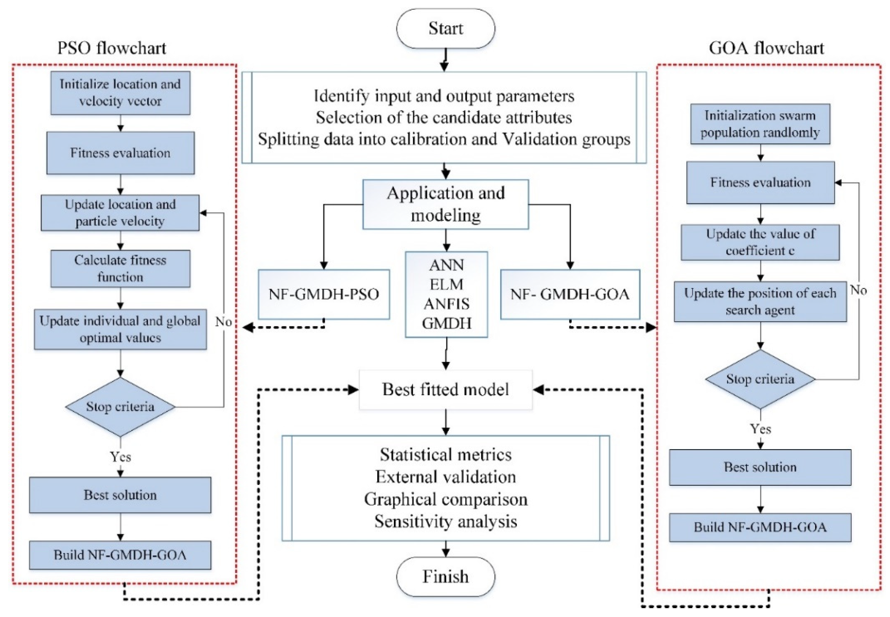
In the present research, various AI techniques like ANN, ELM, ANFIS, GMDH, and hybridized NF-GMDH with HOA/PSO algorithms for modeling of the monthly TDS at two stations were implemented. In this subsection the development of those standalone and hybrid AI models is described in detail. In addition, Figure 1 shows the implementation steps of the workflow of the present research.

2.1. Artificial Neural Network (ANN)

Artificial neural networks (ANNs) are intelligent models derived from biological structures in the brain [37]. ANN models are based on how the neural systems in the human body interact with each other and have a parallel processing architecture. In such a network, nodes (neurons) are connected with links, and layers are structured as nodes and links. Each link is given a specific weight, which can be considered a numerical representation of its strength. The summation value of input weights is transformed into a target using a transfer function, which is typically a sigmoid function. As an example, y can be expressed as follows for the second layer j [38]:

$$y_{pj}={{\displaystyle \sum }}_{i=1}^I{W}_{ij}{O}_{pi}+b_j$$

(1)

In this equation,$O_{pi}$ represents the ith output for the previous layer,$W_{ij}$ represents the weights among layers one and two, and $b_j$ represents the bias of the node j. A nonlinear activation function was used to estimate y, and afterward an output function f(y) was calculated from each node in layers two and three [39].

2.2. Extreme Learning Machine (ELM)

Huang et al. [40] proposed an algorithm, known as Extreme Learning Machine (ELM), that defines hidden nodes’ weights. Model structure selection and model training could be done faster using this approach. In addition, the method is easy to implement since it is relatively simple and straightforward [41]. The i-th output of a network at time t with p input variables, q hidden nodes, and c targets can be calculated as follows:

$$o_i\left(t\right)=m_i^{T}h\left(t\right)$$

(2)

In this equation, $h\left(t\right)ϵ {ℝ}^q$ represents the hidden node vector output related to suggested input pattern $X\left(t\right)ϵ {ℝ}^q$ by a data set ${\left\{X\left(t\right)\right\}}_{t=1}^n$ and $m_i ϵ {ℝ}^q, \forall i ϵ \left\{1, \dots , c\right\}$_, denotes weight vector that makes links between hidden nodes and the i-th output node. Consider Vector h(t) as:

$$h\left(t\right)={\left[f\left(W_1^{T}X\left(t\right)+b_1\right),f\left(W_2^{T}X\left(t\right)+b_2\right),\dots ,f\left(W_q^{T}X\left(t\right)+b_q\right) \right]}^T$$

(3)

In this equation $f\left(.\right)$ represents a sigmoidal activation function, $W_l ϵ {ℝ}^q$ represents the weight vector for the l-th hidden node, and b_l indicates the bias for the l-th hidden node. Weight vectors w_l can be calculated from uniform distributions or random samples from normal distributions. Furthermore, $H=\left[h\left(1\right) h\left(2\right)\dots h\left(n\right)\right]$ is a matrix with a dimension of $q\times n$ where the t-th column represents the output vector of the hidden layer, $h\left(t\right)ϵ {ℝ}^q$, $D=\left[d\left(1\right) d\left(2\right)\dots d\left(\mathrm{n}\right)\right]$ is a matrix with a dimension of $c\times n$ where the t-th column represents the target or desired vector $d\left(t\right)ϵ {ℝ}^c$ associated with the input pattern $x\left(t\right), t=1, \dots , N$, and $M=\left[m\left(1\right) m\left(2\right)\dots m\left(c\right)\right]$ is a matrix with a dimension of $q\times c$, where the i-th column represents the weight vector $m_iϵ {ℝ}^q, i=1,\dots ,c$. Linear mapping is related to these matrices:

$$D=M^{T}H$$

(4)

In this equation, both D and H are known and received from data, while M is determined by applying the Moore–Penrose pseudo-inverse method, as below.

$$M={\left(H{H}^T\right)}^{-1}H{D}^T$$

(5)

Based on the assumption that the number of output nodes and classes are equal, it is possible to determine the class index i* related to a new input pattern applying the following decision rule:

$$i^{*}=arg\underset{i=1,\dots ,c}{\max }\left\{O_i\right\}$$

(6)

where $o_i$ is determined by Equation (5) [42,43].

2.3. Adaptive Neuro-Fuzzy Inference System (ANFIS)

ANFIS is a sub-branch of ANN that combines fuzzy logic principles with neural networks. The ANFIS model was developed by Jang [44] for solving nonlinear functions, predicting chaotic time series, and identifying nonlinear components. By applying the Fuzzy IF–THEN rules of the Takagi–Sugeno fuzzy inference system, ANFIS can build an input-target mapping. ANFIS is popular with engineers because of its fast learning and adaptability characteristics, as well as its capability to capture the nonlinear formation of processes [7,45].

An integral part of ANFIS is the Fuzzy Inference System (FIS). The first layer is fed with inputs and then membership functions (MFs) return fuzzy values. The rule base consists of two sets of Fuzzy IF–THEN rules, which are both Sugeno and Takagi types:

$$\begin{gathered} Rule 1:if x is A_1 and y is B_1, then f_1=p_{1}x+q_{1}y+r_1, \\ Rule 2:if x is A_2 and y is B_2, then f_2=p_{2}x+q_{2}y+r_2, \end{gathered}$$

All nodes in this layer are selected as adaptive nodes by node functions,

$$O_i^1=\mu A_i\left(s\right)$$

(7)

where $O_i^1$ represents the membership function related to $A_i$, while $A_i$ represents a linguistic label. Since Gaussian functions are highly capable of regressing nonlinear datasets, they are frequently used in ANFIS models. According to Equation (8), a value for a Gaussian membership type function ranging from zero to one can be obtained:

$$\mu \left(x\right)=bell \left(x;a_i,b_i,c_i\right)=\frac{1}{1+{\left[\left(\frac{x-c_1}{a_i}\right)\right]}^{b_i}}$$

(8)

In this equation, $x$ represents the input and {$a_i,b_i,c_i$} are considered as the parameters set. Upon entering the second layer, signals are multiplied, and outputs are sent to the subsequent layer. In the third or rule layer, the value for the $i$th node indicates the strength of the rule in relation to other nodes.

Defuzzification is the fourth layer that builds functions for each node. Using the summation of the signals from the previous layer, the last layer calculates the overall output. In order to compute the errors in a model, a threshold limit is considered between the output of the model and actual real values during the training process. As a result of errors greater than the threshold, a gradient descent algorithm is used to update the premise parameters. This process continues until the parameters with error remain below the threshold calculated by two algorithms of least squares or gradient descent [38,46,47].

2.4. Group Method of Data Handling (GMDH)

The first GMDH algorithm was developed by Ivakhnenko. The GMDH is organized in accordance with self-organizing systems. In this model, partial descriptions (PDs) are generated as quadratic polynomials in each node to select the best values for filtering. Additionally, the GMDH uses a tree-like structure to solve highly complex problems as well as to compute the error criteria that should be used as the termination criteria during the training procedure [48,49].

To find an accurate solution to system identification problems, the function $\widehat{f}$ can replace the actual function f. As a result, the final output of a complicated system, $\widehat{y}$, is predicted near observation y for a given model input considered as $X=\left(x_1, x_2, \dots , x_n\right)$. If there is more than one variable in observations, an output variable can be obtained thus:

$$y_i=f\left(x_{i1}, x_{i2}, \dots , x_{in}\right), \left(i=1,2,3,\dots ,M\right)$$

(9)

Therefore, the GMDH model is capable of predicting the final output, ${\widehat{y}}_i$, given $X=\left(x_{i1}, x_{i2}, \dots , x_{in}\right)$ as input vector. In order to find a correlation between the inputs and the output, it is possible to consider the following function:

$${\widehat{y}}_i=\widehat{f}\left(x_{i1}, x_{i2}, \dots , x_{in}\right), \left(i=1,2,3,\dots ,M\right)$$

(10)

In the following equation, the error values resulting from observations and predictions are determined:

$${\displaystyle \sum }_{i=1}^M{\left[\widehat{f}\left(x_{i1}, x_{i2}, \dots , x_{in}\right)-y_i\right]}^2 \to min$$

(11)

In the GMDH model, independent and dependent relationships are expressed as follows:

$$y=w_0+{\displaystyle \sum }_{i=1}^n{w}_i{x}_i+{\displaystyle \sum }_{i=1}^n{\displaystyle \sum }_{j=1}^n{w}_{ij}{x}_i{x}_j+{\displaystyle \sum }_{i=1}^n{\displaystyle \sum }_{j=1}^n{\displaystyle \sum }_{k=1}^n{w}_{ijk}{x}_i{x}_j{x}_k+\dots ,$$

(12)

Additionally, Equation (12) is referred to as the Kolmogorov–Gabor polynomial. Unlike other kinds of polynomials, quadratic polynomials offer a relatively low error, since their weighting coefficients are calculated by the least squares method. Thus, for each pair of input variables $x_i$ and $x_j$, the calculated error value between predictions, $\widehat{y}$, and actual values, $y$, should be minimized. In addition, a number of nodes in each layer are also eliminated with the least-squares method by using this function, which calculates quadratic polynomial performance, $G_i$. The following is the definition of this function:

$$E=\frac{{{\displaystyle \sum }}_{i=1}^M{(y_i-G())}^2}{M} \to min$$

(13)

Creating the regression quadratic polynomial takes into account all possibilities that might exist for two different independent variables. The weighting coefficients are therefore derived using the least squares method. As a general rule, the number of nodes in all layers is calculated by $C_n^2=n\left(n-1\right)/2$, where $n$ is the number of inputs in the prior layer. However, the PDs can be generated in the first layer for different pairs of $p, q \in \left\{1, 2, \dots , n\right\}$ from observation $\left\{\left(y_i{x}_{ip}{x}_{iq}\right);\left(1, 2, \dots , M\right)\right\}$. As a result, $M$ triples $\left\{\left(y_i{x}_{ip}{x}_{iq}\right);\left(1, 2, \dots , M\right)\right\}$ could be built from n observations applying $p, q \in \left\{1, 2, \dots , n\right\}$ as input–output systems. M matrix can be obtained thus [27]:

$$\left[\begin{array}{c}{x}_{1p} x_{1q} y_1\\ x_{2p} x_{2q} y_2\\ . . .\\ x_{mp} x_{mq} y_m\end{array}\right]$$

(14)

Here, the set of quadratic polynomials’ weighting coefficients is $W={\left\{w_0, w_1,\dots , w_5 \right\}}^{Tr}$, and $Y={\left\{y_1, y_2,\dots , y_M \right\}}^{Tr}$ is the output vector. Consequently, the mathematical matrix equation can be defined by AW = Y. As a result, by combining the two inputs, the final matrix can be expressed as:

$$\left[\begin{array}{c}1\\ 1\\ \cdot \\ 1\end{array}\begin{array}{c}{x}_{1p}\\ x_{2p}\\ \cdot \\ x_{mp}\end{array}\begin{array}{c}{x}_{1q}\\ x_{2q}\\ \cdot \\ x_{mq}\end{array}\begin{array}{c}{x}_{1p}\cdot x_{1q}\\ x_{2p}\cdot x_{2q}\\ \cdot \\ x_{mp}\cdot x_{mq}\end{array}\begin{array}{c}{x}_{1p}^2\\ x_{2p}^2\\ \cdot \\ x_{mp}^2\end{array}\begin{array}{c}{x}_{1q}^2\\ x_{2q}^2\\ \cdot \\ x_{mq}^2\end{array}\right]$$

(15)

The coefficients vector of $W={\left(A^{Tr}A\right)}^{-1}{A}^{Tr}Y$ can be obtained by applying the least-squares method [50,51].

2.5. Particle Swarm Optimization (PSO)

In PSO, which is an evolutionary algorithm, an answer to a problem is iteratively optimized to find the best solution. To create a new population, PSO shifts the population positions in every iteration. In addition to affecting individuals’ trajectory, shifting tasks also have an impact on their neighbors’ trajectory. In the search space, the vector x_i represents the position for a particle. This vector represents a possible particle or solution, whose dimension is determined by the number of existing parameters. The parameters, x_i⁰ and v_i⁰, indicate randomly chosen numbers associated with the position and velocity at iteration 0, related to particle i, respectively. Afterward, the vectors of particles are updated according to the fitness function. According to Equations (16) and (17), the vectors are updated [52,53]:

$${\mathrm{v}}_{\mathrm{i}}^{\mathrm{k}+1}={\mathsf{\omega }\mathrm{v}}_{\mathrm{i}}^{\mathrm{k}}+{\varnothing }_1\left({\mathrm{g}}^{\mathrm{k}}-{\mathrm{x}}_{\mathrm{i}}^{\mathrm{k}}\right)+{\varnothing }_2\left({\mathrm{I}}_{\mathrm{i}}^{\mathrm{k}}-{\mathrm{x}}_{\mathrm{i}}^{\mathrm{k}}\right)$$

(16)

$${\mathrm{X}}_{\mathrm{i}}^{\mathrm{k}+1}={\mathrm{X}}_{\mathrm{i}}^{\mathrm{k}}+{\mathrm{V}}_{\mathrm{i}}^{\mathrm{k}+1}$$

(17)

Factors affecting velocity include:

• First, the value of velocity from the prior iteration multiplied by the inertia weight constant, ${\mathsf{\omega }\mathrm{v}}_{\mathrm{i}}^{\mathrm{k}}$,
• Second, the difference between the particle’s current position ${\mathrm{x}}_{\mathrm{i}}^{\mathrm{k}}$ and the best global position ${\mathrm{g}}^{\mathrm{k}}$, which is also known as social learning, and
• Third, the difference between the particle’s current position ${\mathrm{x}}_{\mathrm{i}}^{\mathrm{k}}$ and the local best particle’s position up to this point, ${\mathrm{I}}_{\mathrm{i}}^{\mathrm{k}}$, which is also known as cognitive learning.

The second and third factors are influenced by equations ${\varnothing }_1={ \mathrm{c}}_1{\mathrm{r}}_1$, ${\varnothing }_2={ \mathrm{c}}_2{\mathrm{r}}_2$. In these equations, r_x represents a real randomly selected number of a uniformly distributed function between [0,1], and c_x represents a constant value for x = 1,2. The particles cover the entire search space in the first iteration. With the increase in the number of iterations, the search space decreases. Therefore, PSO analyzes plausible zones first and ultimately improves its best solution. Over the years, there have been several versions of PSO in the literature. In this study, the standard version of PSO proposed in 2011 with the subsequent parameters was chosen:

$$\omega =\frac{1}{2ln2} and c_1=c_2=0.5+ln2$$

(18)

Swarm topology determines how particles communicate with each other on a global scale by defining their connectivity and how they exchange information with each other. Communication between particles usually involves three (k) random particles [30].

2.6. Grasshopper Optimization Algorithm (GOA)

A grasshopper swarm algorithm, developed by Saremi et al. [54], simulates natural grasshopper swarm behavior and is used in many different engineering fields. Adult grasshoppers and nymphs (larvae) both engage in swarming behavior. The swarm behavior of grasshoppers has two key characteristics: first, exploration and exploitation to find food sources; and second, the movement of grasshoppers, including the slow movement of larvae and the long, abrupt movements of adults. The search agents tend to move abruptly during exploration, although their behavior develops local movement during exploitation [55,56].

It is the adults’ responsibility to explore the entire search space and discover suitable food sources (exploration), while the nymphs work at exploiting a specific region or neighborhood in a particular position (exploitation) [54]. Through this algorithm, exploration and exploitation phases are smoothly balanced and mathematically incorporated into a less complex algorithm structure. According to this algorithm, the following steps are taken [12]:

Step 1: First, for GOA, a population of size S_c is generated by applying Equation (19).

$$X_{kj}=X_{kj}+rand\left(0,1\right).\left(\overline{X_{kj}}-\underset{¯}{X_{kj}}\right) \forall k\in S_c; \forall j\in N$$

(19)

where S_c indicates the population size and N represents the problem’s dimension. Moreover, l_j and u_j are the lower and upper limits for the jth variable.

Step 2: Based on the fitness value, the best position can be determined in this step.

$$fit\left(x_j\right)=\frac{1}{1+f\left(x_j\right)}$$

(20)

In this equation f(x_j) is the fitness function, which in this article is the Mean Square Error (MSE).

Step 3: The exploitation and exploration parameters of the GOA are balanced with the c parameter, which can change over time, depending on the number of iterations (iter). The c parameter is calculated by:

$$c=c_{max}-iter.\frac{c_{max}-c_{min}}{M_I}$$

(21)

In this equation, M_I is the maximum value of the cycle number.

Step 4: By applying Equation (22), the new positions can be obtained.

$$c{X}_i^d=c.\left\{{{\displaystyle \sum }}_{\begin{array}{c}j=1\\ j\ne i\end{array}}^{S_c}c.\frac{\overline{X_i}-\underset{¯}{X_i}}{2}.s\left(\left|X_j-X_i\right|\right).\frac{X_j-X_i}{d_{ij}}\right\}+T_d \forall i\in N$$

(22)

where $s\left(r\right)$ is:

$$S\left(r\right)=f.e^{\left(-\frac{r}{l}\right)}-e^{-r}$$

(23)

In these equations, f represents the attraction intensity, T_d indicates the best discovered solution, and l represents the attraction length. According to Equation (22), the normalized distance between the best discovered solution and the real search space position can be determined. The better position is saved after evaluating the newfound position with Equation (21). It should be noted that Equation (22) is modified by changing the c parameter, resulting in later iterations focusing on exploration and earlier iterations focusing on exploitation. Algorithm accuracy is improved by using this tuning procedure.

Step 5: In the final step, the algorithm is repeated considering a counter known as the iteration counter (iter).

Step 6: The optimization is complete when the number of iterations (iter) gets to the maximum loop number (MI).

2.7. Development of an Adaptive Fuzzy-GMDH Using PSO/GOA

Ivakhnenko created the GMDH neural network, which is a type of self-organizing model that can perform a variety of processes. An integration of input parameters, based on the complex theorem of Ivakhnenko, is introduced in the first operation to build PDs or polynomial neurons [57]. The seeds selection is done in the second operation regarding error criteria, depending on the filtering process in each layer. Moreover, this is done using the means of evolutionary computing methods, which, combined with parallel mechanisms, leads to the enhancement of the optimal NF-GMDH structure. As a matter of significant importance, NF-GMDH model is flexible enough to be effectively applied as a conjunction model by other evolutionary and iterative algorithms [27].

A review of the literature showed that the Gaussian membership function, $F_{kj}$, has been extensively used for building neural-Fuzzy systems due to producing more accurate results in the NF-GMDH model. Indeed, the number ($k$) of Fuzzy rules is introduced by $F_{kj}$ which is applied in the bound of the $j$th input vector ($x_j$):

$$F_{kj}\left(x_j\right)=EXP[\frac{{\left(x_j-a_{kj}\right)}^2}{b_{kj}}]$$

(24)

where actual values of $b_{kj}$ and $a_{kj}$ indicate the constant coefficients of the Gaussian membership function called the Fuzzy rule. Moreover, output vector, $y$, is computed as the result of a neural-Fuzzy network using Equation (25):

$$y={{\displaystyle \sum }}_{k=1}^K{u}_k{w}_k$$

(25)

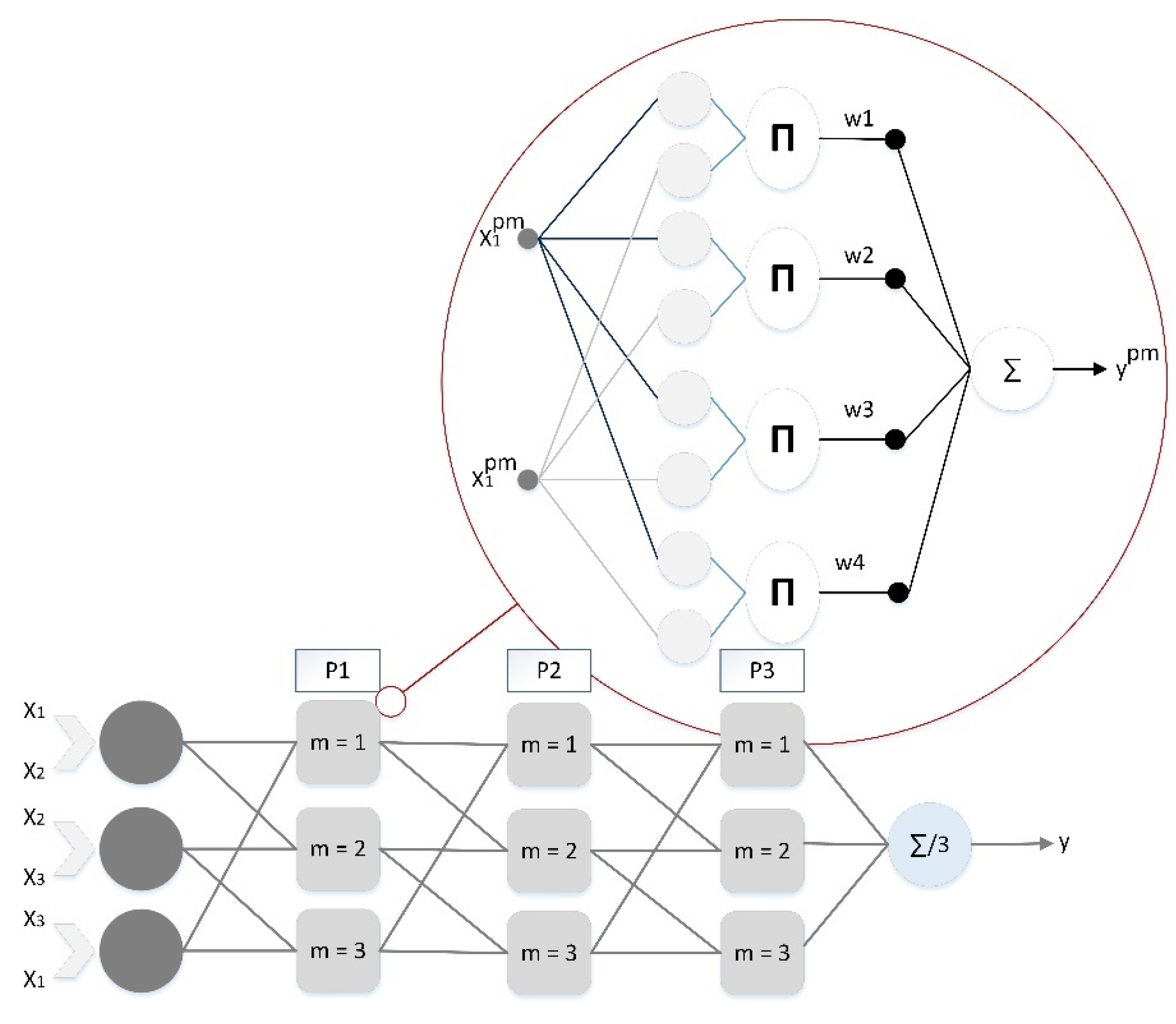
where $w_k$ and $u_k={\displaystyle \prod }_j{F}_{kj}\left(x_j\right)$ are the observed values for $k$th Fuzzy rules. Each PD or neuron has mainly one output and two inputs through the NF-GMDH model. As seen in Figure 2, the input vector in the next layer is the output vector for each PD in the current layer. The average of outputs in the last layer gives the final output of the NF-GMDH method. The inputs from the $p$th layer and the $m$th neuron in the $p-1$ layer are considered as the output of the $m-1$th and $m$th PDs which create input vector in the $p$th layer$\mathrm{and}$ $m$th PD. The mathematical relationship between $y^{p-1, m-1}$, $y^{p-1,m},$ and $y^{pm}$ is obtained from Equation (26):

$$y^{pm}=f\left(y^{p-1,m-1},y^{p-1,m}\right)={{\displaystyle \sum }}_{k=1}^K{\mu }_k^{pm}.w_k^{pm}$$

(26)

where ${\mu }_k^{pm}$ is a mathematical expression to compute the $k$th Gaussian function. Finally, the NF-GMDH network output is as below:

$$y=\frac{1}{M}{{\displaystyle \sum }}_{m=1}^M{y}^{pm}$$

(27)

The trial–error process computes the weighted coefficients and Gaussian functions [57,58].

In the hybrid NF-GMDH model, associated parameters in partial descriptions act as a form of Gaussian function. Fuzzy MFs parameters need to be tuned using a back-propagation algorithm. This conventional trainer has a vital problem wherein this algorithm cannot find which PD or link desires to be excluded; hence, the network structure has some needless PDs and links. For tuning and optimization of Fuzzy MFs parameters, as well as attaining optimal weighting coefficients related to PDs in GMDH over the NF-GMDH model’s complex topology, an effective and robust algorithm is essential. In the present study, the GOA algorithm is applied due to its superiority in exploitation and exploration for seeking the best solution for complex problems. This novel approach has the potential to be simultaneously implemented for training network parameters and structural identification [16,57].

Adjustable variables in the GOA algorithm can control the best solution to provide minimum difference from the objective function. Equation (28) is the objective function of the optimization operation in the NF-GMDH based on GOA:

$$Eval=\frac{{{\displaystyle \sum }}_{i=1}^N{\left(y\left(i\right)-\widehat{y}\left(i\right)\right)}^2}{N}$$

(28)

Table 1. Initial parameter of the proposed algorithms.

Algorithm	Parameters	Value
PSO	Acceleration constant (C1 and C2)	2
	Inertia Wmax	0.9
	Inertia Wmin	0.4
	Number of particles	50
GOA	Seeking memory pool	5
	Counts of dimension to change	0.8
	Seeking rang of the selected dimension	0.2
	Mutative ratio	0.9

shows the values of the GOA and PSO algorithms’ setting parameters. All weighting factors are determined after the model optimization. Consequently, NF-GMDH based on GOA and PSO gives the Gaussian functions.

2.8. Case Study Description

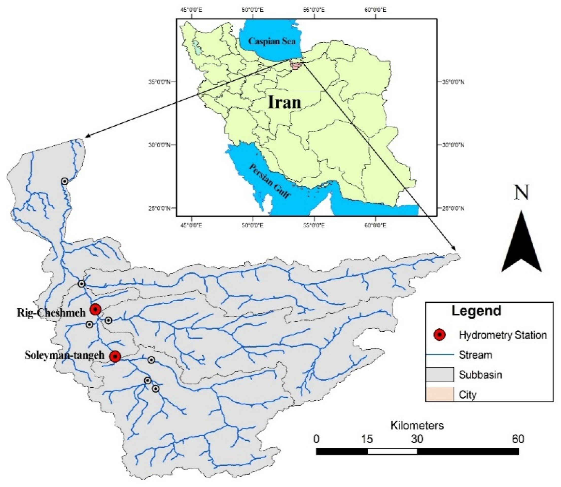
The Tajan River basin, as a river in Mazandaran, has a mostly humid or semi-humid climate. The annual rainfall, average river discharge, and area slope are 539 mm, 20 m³/s, and 85%, respectively. The difference between minimum and maximum level of the Tajan basin is approximately 3700 m; 90% of the forest surface is covered by brown soil and the remainder is covered by widespread types such as alluvial soil [6] Various agricultural, aquacultural, aquafarming, and industrial activities are implemented in this river basin. Moreover, different operations, including damming and sand mining, are done in the river, which affect the average amount of measured TDS. Due to the high rate of rainfall and the beginning of agricultural production, TDS monitoring is needed annually in the fall and winter [23]. In the basin, there are nine active hydrometric gauging stations. For TDS modeling, data from the Soleyman Tange and Rig-Cheshme stations were collected as shown in Figure 3.

The characteristics of the physiochemical parameters of the case study are shown in

Table 2. Monthly averages of statistical indices of the Tajan basin.

Variables	Indices	Rig-Cheshmeh	Soleyman-Tangeh
HCO3 (mg/L)	Min	1.6	1.2
	Mean	3.88	1.2
	Max	12.2	0.5
	Std	0.89	0.08
	Variation	0.79	156
Ca (mg/L)	Min	1.1	3.84
	Mean	3.16	3.41
	Max	7.5	2.07
	Std	0.68	0.87
	Variation	0.46	408.87
Mg (mg/L)	Min	0.1	7.7
	Mean	2.17	6.3
	Max	6	4.5
	Std	0.69	2.94
	Variation	0.48	650
Na (mg/L)	Min	0.2	0.91
	Mean	1.54	0.66
	Max	6.5	0.68
	Std	0.75	0.42
	Variation	0.57	63.1
TDS (mg/L)	Min	271	0.83
	Mean	446.49	0.44
	Max	1270	0.46
	Std	78.7	0.18
	Variation	6194.38	3981.8

. TDS reached its peaks at two suggested stations based on observations (Rig-Cheshmeh (1270) and Soleyman-Tangeh (650)). According to Table 1, the standard deviation of TDS records was distributed over a wide range compared to input variables. Although there are various parameters which have a significant effect on TDS estimating, monthly magnesium (Mg), calcium (Ca), bicarbonate (HCO₃), and sodium (Na), which are provided from the Meteorological Organization of Mazandaran Province (MOMP) during March 1984–August 2016 and March 1974–August 2016 at Soleyman-Tangeh (390 monthly data record) and Rig-Cheshmeh (505 monthly data record) gauging stations, respectively, were used in the TDS modeling. In this regard, about 75% of the total dataset was used for training and the rest was set aside for testing the AI’s networks.

2.9. Model Performance Criteria

For assessing the model’s robustness, correlation coefficient (R), root mean square error (RMSE), Nash-Sutcliffe efficiency (NSE), and ratio of RMSE to standard deviation (RSD) were used,

$$R=\frac{{{\displaystyle \sum }}_{i=1}^N\left(T_{obs}-\overline{T_{obs}}\right).\left(T_{pre}-\overline{T_{pre}}\right)}{\sqrt{{{\displaystyle \sum }}_{i=1}^N{(T_{obs}-\overline{T_{obs}})}^2{{\displaystyle \sum }}_{i=1}^N{\left(T_{pre}-\overline{T_{pre}}\right)}^2}}$$

(29)

$$RMSE=\sqrt{\frac{1}{N}{{\displaystyle \sum }}_{i=1}^N{\left(T_{pre}-T_{obs}\right)}^2}$$

(30)

$$NSE=1-\frac{{{\displaystyle \sum }}_{i=1}^N{\left(T_{pre}-T_{obs}\right)}^2}{{{\displaystyle \sum }}_{i=1}^N{\left(T_{obs}-\overline{T_{obs}}\right)}^2}$$

(31)

$$RSD=\frac{RSME}{{{\displaystyle \sum }}_{i=1}^N\left(T_{obs}-\overline{T_{obs}}\right)}$$

(32)

In the above equations $T_{obs}$ and $T_{pre}$ represent the observations and predictions, respectively. $\overline{T_{obs}}$ and $\overline{T_{pre}}$ are the means of the observations and predictions, respectively. The R index was used for selecting suitable predictors for predicting the target variable. In addition, N stands for the total number of datasets. NSE evaluates the model’s output using a set of (−∞, 1) and an ideal value of unity. As a result, perfect fitting between observations and predictions has NSE equal to 1, and NSE with a negative value indicates that the model performs poorly in terms of the arithmetic mean of the models tested. With a range of (0 to +), RSD and RMSE are calculated, and an ideal value of zero indicates the model accuracy.

After model optimization, the testing dataset is used for the model validation. Validation measures are adopted in this study [59]. For the projections based on observations, the gradients of the regression line through the origin (k), or for the predictions via observations (k′), at least one needs to be near to 1.

$$k={{\displaystyle \sum }}_{i=1}^n\left(T_i\times P_i\right)/P_i^2 or k^{\prime }={{\displaystyle \sum }}_{i=1}^n\left(T_i\times P_i\right)/T_i^2$$

(33)

Additionally, the coefficient of determination for the regression lines through the origin m′ and n′ should be less than 0.1.

$$m^{\prime }=\left(R^2-R_O^2\right)/R^2 \mathrm{and} n^{\prime }=\left(R^2-{R_O^{\prime }}^2\right)/R^2$$

(34)

Moreover, the cross-validation coefficient R_m should satisfy:

$$R_m=R^2\times \left(1-\sqrt{\left|R^2-R_O^2\right|}\right) > 0.5$$

(35)

Between the observed and predicted values, the determination coefficients through the origin ${R_O^{\prime }}^2$ and conversely (the estimated and observed values) $R_O^2$ are calculated thus:

$$\begin{gathered} R_O^2=1-{{\displaystyle \sum }}_{i=1}^n{P}_i^2{\left(1-k\right)}^2/{{\displaystyle \sum }}_{i=1}^n{\left(P_i-\overline{P}\right)}^2 \& \\ {R_O^{\prime }}^2=1-{{\displaystyle \sum }}_{i=1}^n{T}_i^2{\left(1-k^{\prime }\right)}^2/{{\displaystyle \sum }}_{i=1}^n{\left(T_i-\overline{T}\right)}^{2 } \end{gathered}$$

(36)

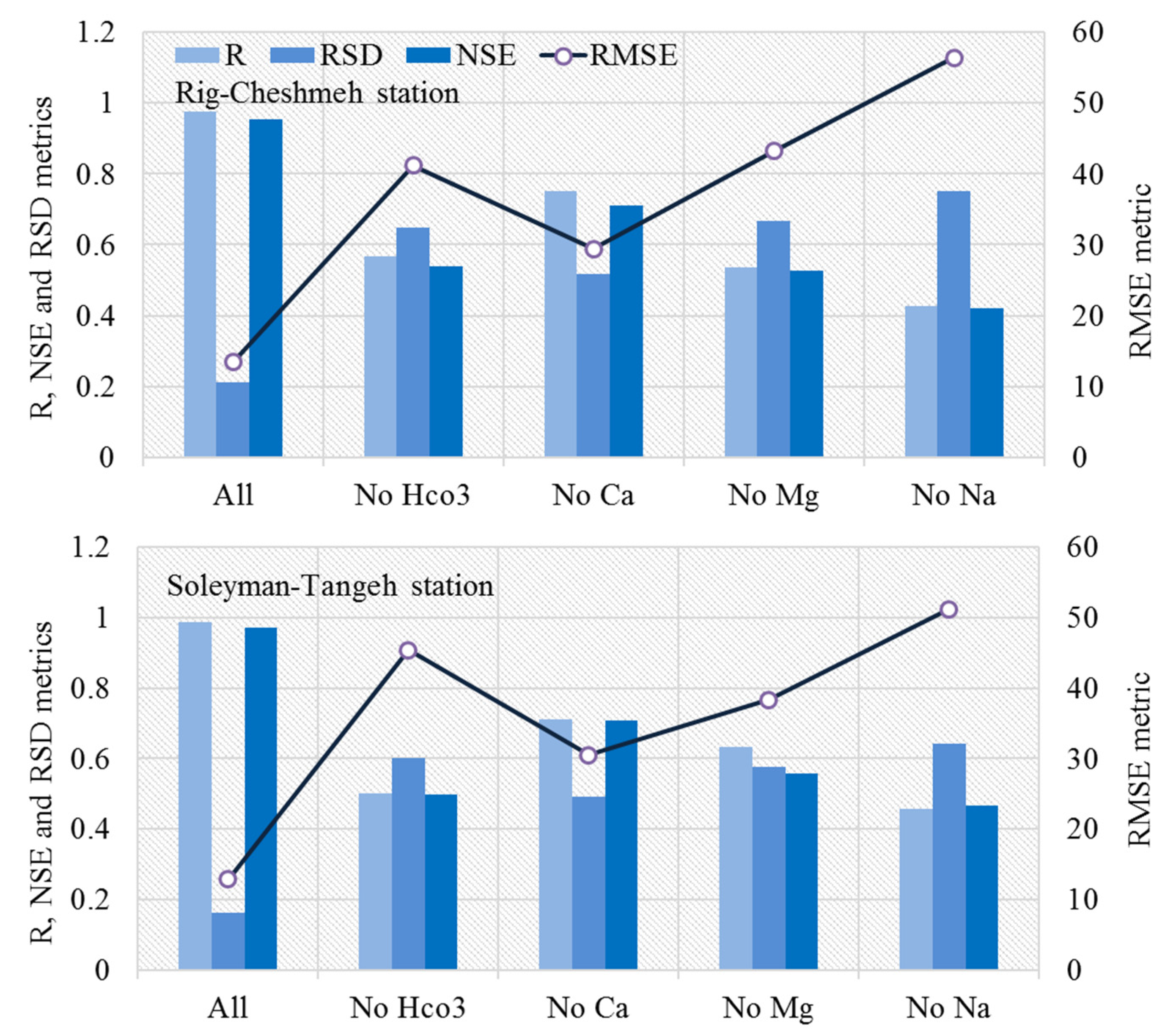
A sensitivity analysis may be used to assign the effect of input variables on TDS using the best suited model. In this study, one input variable parameter was eliminated at a time to assess the impact of that input on output. The following relationships are used to measure the percentage of sensitivity of each output variable to each input variable:

$$N_i=f_{max}\left(x_i\right)-f_{min}\left(x_i\right)$$

(37)

$$S_i=\frac{N_i}{{{\displaystyle \sum }}_{j=1}^n{N}_j}\times 100$$

(38)

where $f_{max}\left(x_i\right)$ is the maximum and $f_{min}\left(x_i\right)$ is the minimum of the predicted output over the ith input domain, whilst other variables have mean values.

3. Results and Discussion

3.1. Performance Results of Standalone and Hybrid Models

3.1.1. The Case Study of Rig-Cheshmeh Station

Monthly TDS was modeled based on data collected from the Rig-Cheshmeh gauging station. The performance of proposed techniques for forecasting TDS in calibration and validation stages is shown in

Table 3. Statistical evaluation of proposed models at calibration and validation stages for Rig-Cheshmeh station.

	ANN	ELM	ANFIS	GMDH	NF-GMDH-PSO	NF-GMDH-GOA
Calibration
R	0.947	0.975	0.973	0.968	0.980	0.986
RMSE (mg/L)	29.991	18.053	22.222	20.784	16.099	13.478
RSD	0.369	0.222	0.273	0.256	0.198	0.166
NSE	0.864	0.951	0.925	0.934	0.961	0.972
Validation
R	0.906	0.935	0.970	0.924	0.962	0.985
RMSE (mg/L)	27.178	22.439	14.975	24.579	20.564	10.744
RSD	0.440	0.363	0.242	0.398	0.333	0.174
NSE	0.805	0.867	0.941	0.840	0.888	0.970

.

Evidently, integrated NF, GMDH, and GOA (NF-GMDH-GOA) yielded the best prediction (i.e., largest R, as well as lowest RMSE) in comparison to other models, indicating integrating proposed approaches can be considered as a robust modeling approach for non-stationary evaluation and increasing the accuracy of the model for Rig-Cheshmeh station in calibration and validation stages. The integrated NF-GMDH and GOA algorithm had the best predictive ability, rather than other hybrid methods, based on the performance criteria (lowest RMSE = 13.478 mg/L, NSE = 0.972, R = 0.986, and RSD = 0.166). The NF-GMDH-PSO model with higher errors in terms of RMSE (19.44%) and RSD (1.131%) ranked next in this study.

The standalone ANN, ELM, ANFIS, and GMDH models and combined approaches (NF-GMDH-PSO and NF-GMDH-GOA) were employed in the validation stage (Table 3). The evaluation metrics of the NF-GMDH-GOA model with respect to RMSE (10.744 mg/L) and NSE (0.970) outperformed other models such as ELM (RMSE = 22.439 mg/L and NSE = 0.867) and ANN (RMSE = 27.178 mg/L and NSE = 0.805). Additionally, among the proposed models, ANFIS achieved higher accuracy compared to the other approaches.

The coefficient of determination and the Pearson’s correlation coefficients (R) between TDS observations and predictions are shown in Figure 4. The scatterplots exhibit the agreement between predictions and observations. For each sub-panel, the determination coefficient (R²) and least-squares regression (LSR) were presented.

As illustrated in Figure 5 for the Rig-Cheshmeh station, NF-GMDH-GOA successfully predicted the TDS variations; therefore, it is recommended as the best model. Figure 5 demonstrates the error plots of TDS observations via predictions and their time series during calibration and validation stages at the Rig-Cheshmeh station. Obviously, NF-GMDH-GOA was confirmed to be a potential model to model the TDS variations (especially peak values), while ANN underestimated the peak values, representing the weak performance ability of this model in TDS predicting in the Tajan river basin in the case study. Moreover, the minimum variation of errors of TDS measured and estimated by NF-GMDH-GOA was between −100 and 100. On the other hand, these variations for other alternative approaches were out of that interval. For example, the error variation of the GMDH model was from −200 to 300.

3.1.2. The Case Study of Soleyman-Tangeh Station

This process was conducted for data obtained from the Soleyman-Tangeh gauging station as presented in

Table 4. Statistical evaluation of proposed models at calibration and validation stages for Soleyman-Tangeh station.

	ANN	ELM	ANFIS	GMDH	NF-GMDH-PSO	NF-GMDH-GOA
Calibration
R	0.891	0.950	0.932	0.948	0.948	0.973
RMSE (mg/L)	40.295	19.538	22.807	19.938	20.107	14.376
RSD	0.640	0.310	0.362	0.317	0.320	0.228
NSE	0.589	0.903	0.868	0.899	0.898	0.948
Validation
R	0.817	0.905	0.781	0.892	0.975	0.989
RMSE (mg/L)	27.823	19.378	35.364	22.254	10.113	9.687
RSD	0.655	0.456	0.833	0.524	0.238	0.223
NSE	0.567	0.790	0.300	0.723	0.942	0.948

. Results showed that the integrated model (NF-GMDH-GOA) significantly improved the performance of all metrics (R, RMSE, NSE, and RSD). Therefore, NF-GMDH-GOA was superior to other models with the lowest error (RMSE = 14.376 mg/L and RSD = 0.228) and highest predictive power (NSE = 0.948, and R = 0.974). Conversely, ANN performed poorly, with significant difference in RMSE (40.295 mg/L) and NSE (0.589) compared to ANFIS (RMSE = 22.807 mg/L and NSE = 0.868) and GMDH (RMSE = 19.938 mg/L and NSE = 0.899), and showed insufficient performance for the WQP modeling in the calibration stage.

At the validation stage, evaluation metrics proved that NF-GMDH-GOA had the highest potential to model TDS compared to other modeling approaches. The computed value of NSE rose from 0.723 to 0.948 for the GMDH model. Similarly, the RSD and RMSE decreased by 0.223 and 9.687 mg/L, respectively.

Moreover, the scatter plots of TDS observations, via predictions and observations, are presented in Figure 6 for the Soleyman-Tangeh station. The obtained slope lines of the TDS values for NF-GMDH-GOA model were near to the best-fitting line; however, some TDS values were underestimated. The ANN and ANFIS models could not estimate the WQP parameter more precisely than the other models, and this indicates the poor performance of these models for TDS modeling.

At the Soleyman-Tangeh station, the feasibility results of the proposed NF-GMDH-GOA showed the highest accuracy regarding general tendency and ability in prediction of the TDS peaks (Figure 7). In addition, ANN and ANFIS had poor performance for the TDS modeling, demonstrating that these models were incapable of predicting TDS variations. Therefore, integrated AI methods had more ability than standalone models in TDS prediction. In terms of error plot: it can be concluded that the minimum interval (−100 to 100) and maximum interval (−200 to 200) of variation error were obtained by the ANN and NF-GMDH-GOA techniques, which illustrated the high capability of the integrated model (NF-GMDH-GOA) in TDS forecasting.

3.2. Further Analysis and Discussion

The external validation associated with the proposed artificial intelligence models by the relevant criteria is summarized in

Table 5. External validation statistical measures for forecasting TDS using AI models.

Metrics	ANN	ELM	ANFIS	GMDH	NF-GMDH-PSO	NF-GMDG-GOA
Rig-Cheshmeh station
R (R > 0.8)	0.906	0.935	0.97	0.924	0.962	0.985
K (0.85 < K < 1.15)	1.017	1.001	0.997	1.003	0.975	1.002
K′ (0.85 < K′ < 1.15)	0.979	0.996	1.001	0.994	1.024	0.998
m (m < 0.1)	−0.202	−0.143	−0.062	−0.171	−0.047	−0.03
n (n < 0.1)	−0.185	−0.142	−0.062	−0.17	−0.042	−0.03
Rm (Rm > 0.5)	0.48	0.565	0.714	0.527	0.732	0.804
Soleyman-Tangeh station
R (R > 0.8)	0.817	0.905	0.781	0.892	0.975	0.989
K (0.85 < K < 1.15)	0.965	0.987	0.943	1.026	1.004	1.022
K′ (0.85 < K′ < 1.15)	1.031	0.101	0.055	0.972	0.996	0.979
m (m < 0.1)	−0.36	−0.206	−0.226	−0.191	−0.051	0.013
n (n < 0.1)	−0.301	−0.212	−0.211	−0.116	−0.051	0.015
Rm (Rm > 0.5)	0.341	0.483	0.384	0.485	0.741	0.866

. As presented in Table 5, NF-GMDH-GOA’s performance was compromisingly satisfied with K = 1.002 and R_m = 0.804 at the Rig-Cheshmeh station, and achieved the best results in selecting the most accurate model in comparison with other models. However, although the values of n, m, K, and K′ of the ANN model were in agreement with the required conditions, the criterion of the $R_m$ value ($R_m$ = 0.487) was obtained as marginally less than 0.5 and subsequently the condition was not met. In terms of R_m and R-values, ANFIS was able to capture TDS variations with an acceptable level of validated criteria, rather than ELM and GMDH.

In addition, Table 5 indicated that integrated NF-GMDH with the GOA algorithm could provide more accurate values for TDS for the Soleyman-Tangeh station, on the basis of criteria values, when compared with PSO. According to the outcomes of external validation, the m and n values given by NF-GMDH-GOA were fixed at 0.013 and 0.015, for NF-GMDH-PSO both m and n were obtained as −0.051, and the other alternative models such as ELM and GMDH were not able to produce TDS predictions with acceptable R_m as external validation criteria. Table 5 presents criteria of R_m for the proposed ANN, ELM, ANFIS, and GMDH approaches, which were 0.341, 0.483, 0.384, and 0.485, respectively. In general, statistical indices have shown the high performance of the NF-GMDH-GOA model in TDS estimation.

Moreover, a sensitivity analysis approach was employed to define the independent variables which have the highest influence on the dependent variables. Similar to the quantitative comparisons, NF-GMDH-GOA model had the highest accuracy for TDS modeling. Hence, four input variables, namely HCO₃, Ca, Mg, and Na, have been considered whose output was WQP, predicted by NF-GMDH-GOA with the highest accuracy.

The primary model was built using all input parameters and then, one of the parameters was removed, and modeling performance was determined to evaluate the effect of each parameter on targets. To study the relationship between input variables and TDS, statistical criteria including R, RMSE, RSD, and NSE parameters were applied. The results of error benchmarks have been summarized in Figure 8. The results demonstrate that among the independent variables, Na with maximum value of error (RMSE = 56.4 mg/L & NSE = 0.752) was the most significant parameter in the TDS modeling. Conceivably, Mg with RMSE = 43.251 mg/L and RSD = 0.668 stood second.

As seen in Figure 8, error criteria showed that Na with the lowest value of accuracy (R = 0.426) had the highest influence on the TDS estimation for the Rig-Cheshmeh station. By removing Na from the model, other criteria included RMSE, RSD, and NSE for TDS modeling, which were 56.404 mg/L, 0.752, and 0.421, respectively. Similar to what was found in the Rig-Cheshmeh station, Na with R (0.458) and RMSE (51.254 mg/L) was the most important parameter in TDS prediction for the Soleyman-Tangeh station. According to the sensitivity result, the main factor which may have contributed to the large amount of Na is the land use in, and land cover of, the area. In the downstream part of the region, which covers the agricultural sectors, due to the use of chemical fertilizers, the amount of Mg in this region essentially contributes to TDS. In general, contributors for the Na and Mg that cause water quality pollution in this region are the use of rivers to transport urban and industrial wastewater and the drainage of agricultural and horticultural fields.

To compare the difference between two models’ means,

Table 6. Results of Wilcoxon signed-rank test between the proposed integrative NF-GMDH-GOA and other models.

Number	Pairwise Comparison	Z	p (<0.05)	Significance
1	NF-GMDH-GOA vs. ANN	−4.496	0.003	Yes
2	NF-GMDH-GOA vs. ELM	−5.621	0.001	Yes
3	NF-GMDH-GOA vs. ANFIS	−7.255	0.001	Yes
4	NF-GMDH-GOA vs. GMDH	−7.158	0.002	Yes
5	NF-GMDH-GOA vs. NF-GMDH-PSO	−8.157	0.001	Yes

tabulates the Wilcoxon signed-rank test results as the nonparametric statistical hypothesis test at a significance level equal to 0.05 on the standalone and hybrid TDS predictive models. As a result, the Z value for those six AI models was greater than the critical Z. The P value calculated for the models should be less than 0.05 which shows the standard significance level. According to the results, the null hypothesis is rejected and the performance of the AI models in the prediction of monthly TDS is significantly different.

4. Concluding Remarks

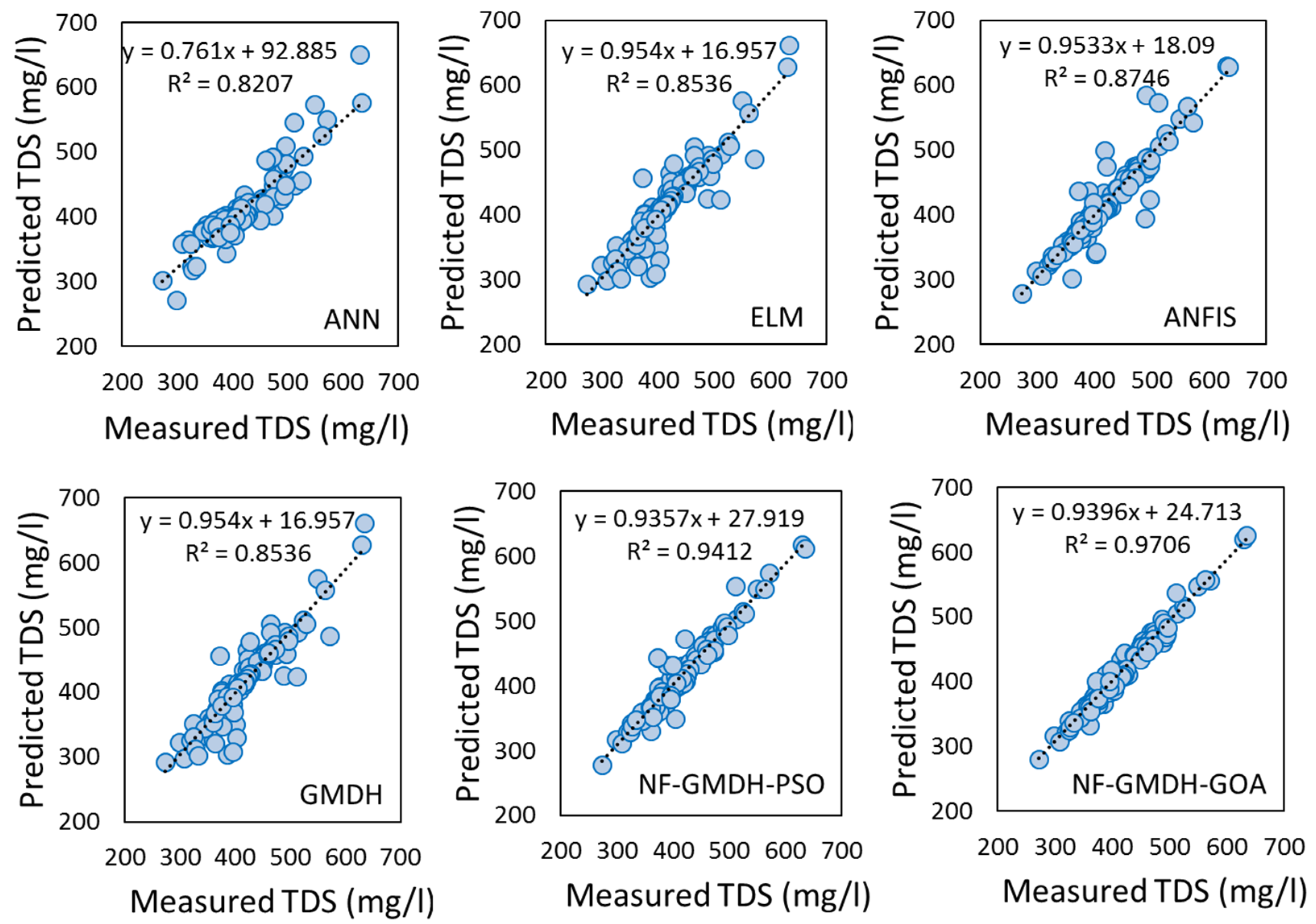
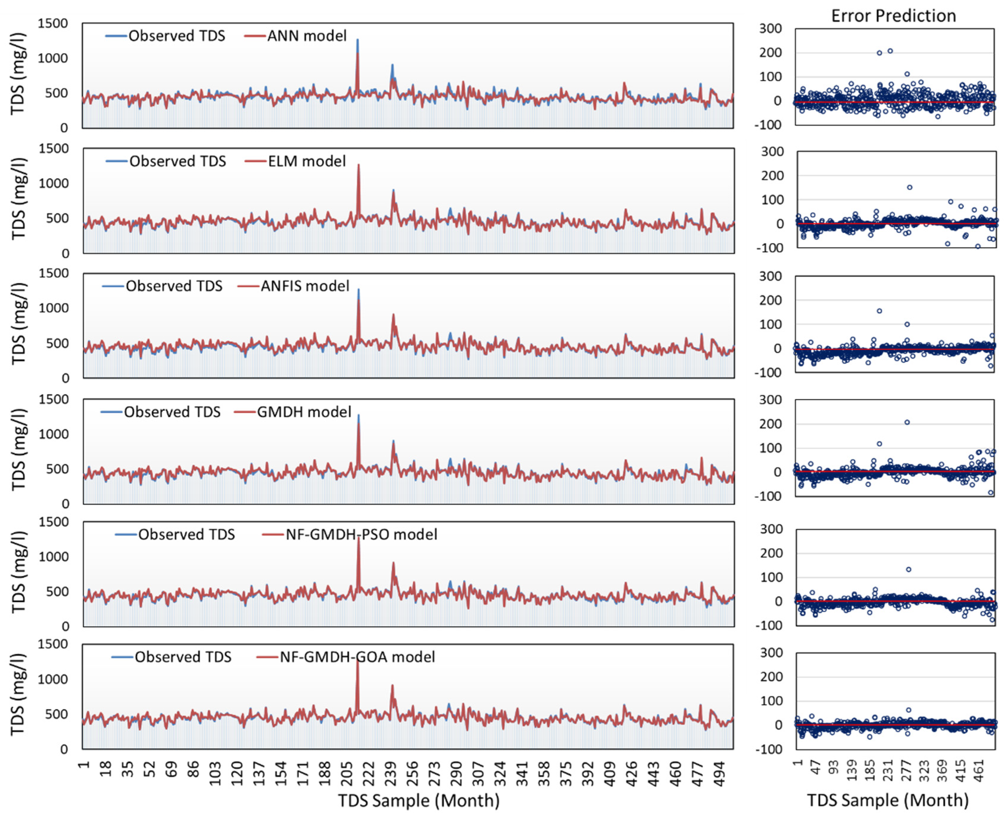
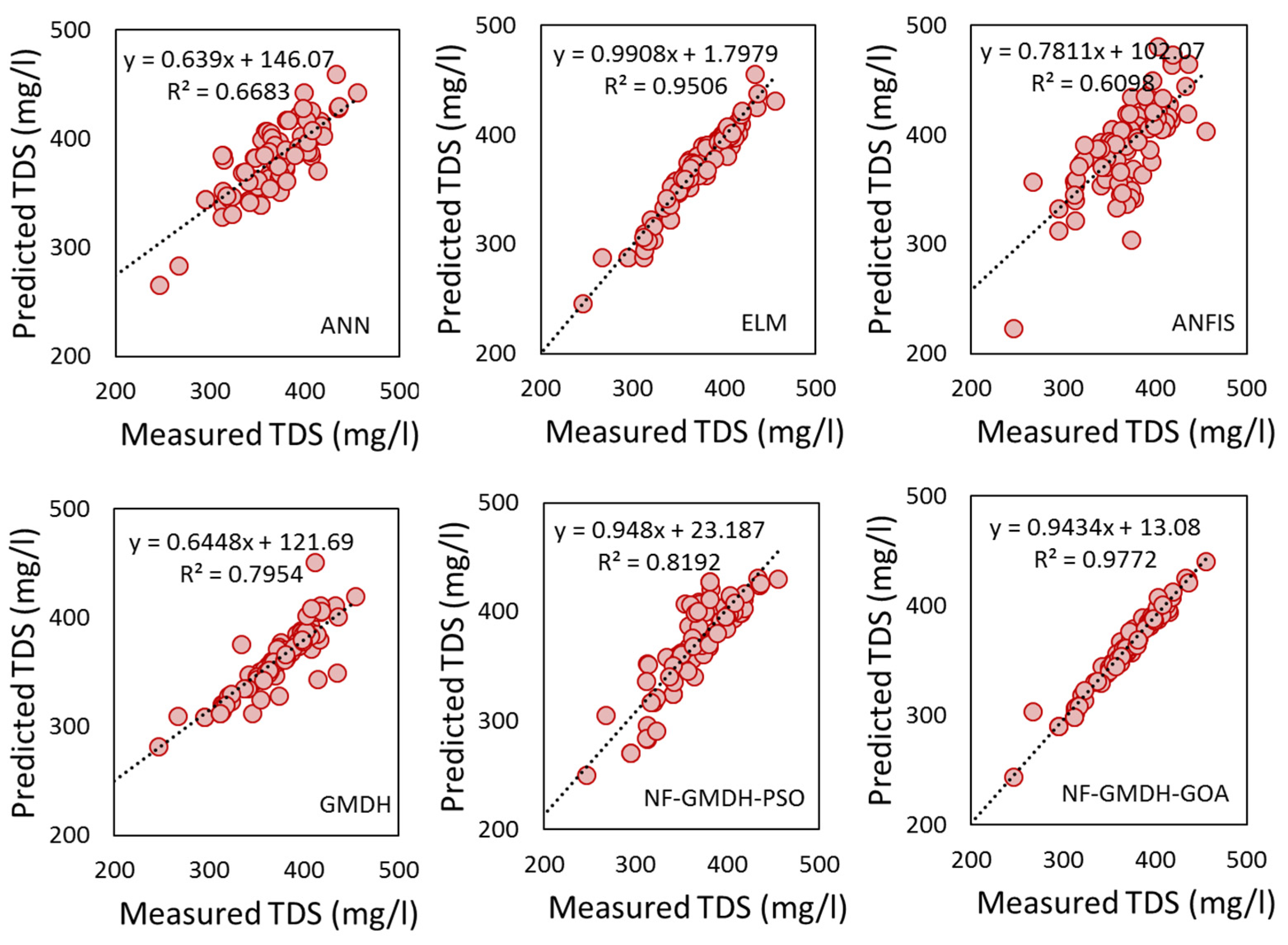
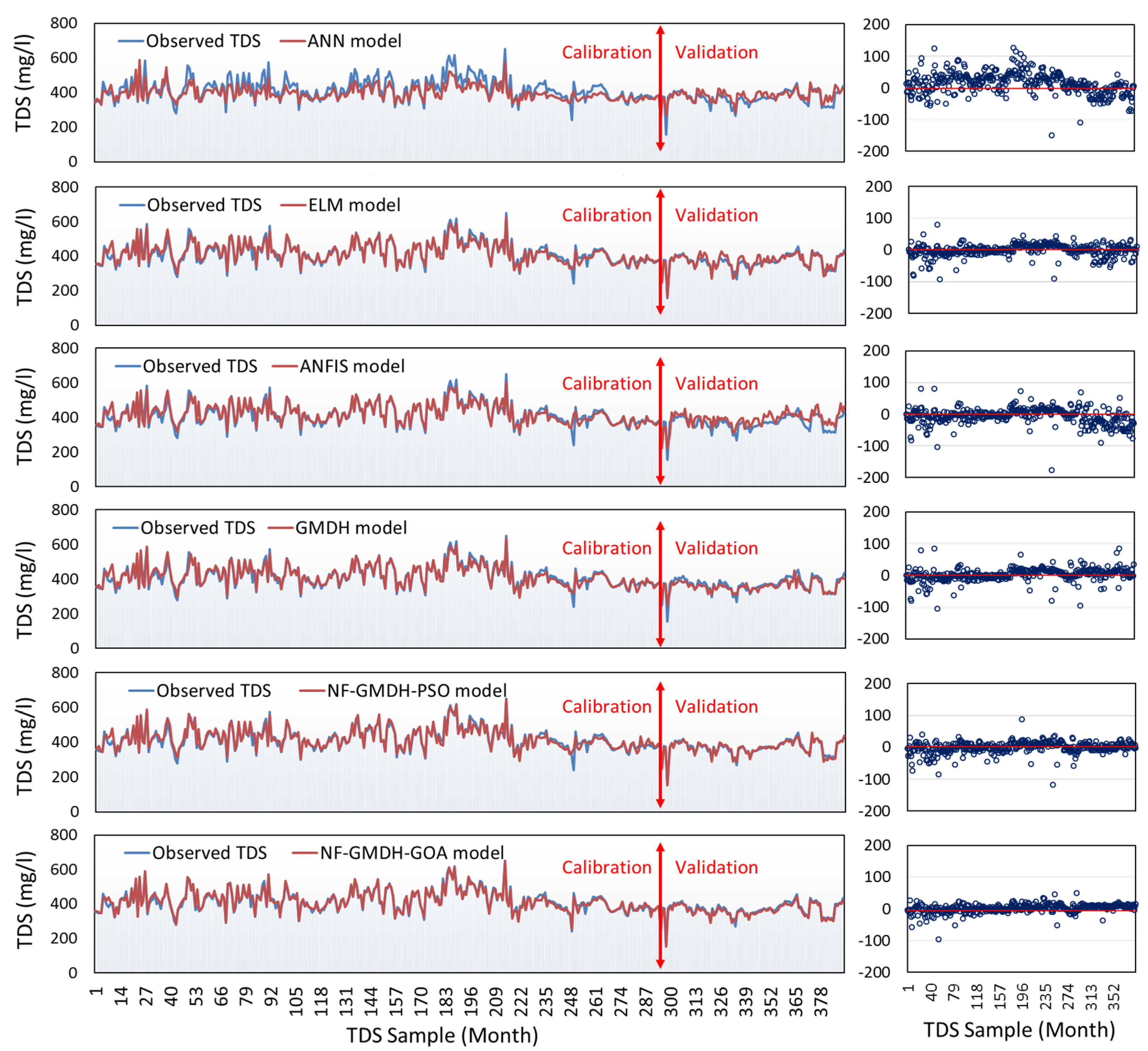
In this study, the capability of the neuro-fuzzy group method of data handling systems-based grasshopper optimization algorithm (NF-GMDH-GOA) was studied in forecasting monthly TDS at the Soleyman-Tangeh and Rig-Cheshmeh stations located in the Tajan River basin, Iran. The most significant parameters of water quality, such as Ca, Mg, Na, and HCO₃, were included in the model. Comparing the results of the hybrid and standalone models showed that the grasshopper optimization algorithm has a major effect on the performance of NF-GMDH. At the Soleyman-Tangeh station, NF-GMDH-GOA could predict TDS with more accuracy in terms of NSE (0.948), RSD (0.223) and RMSE (9.687 mg/L) in comparison to other models at the validation stage. The accuracy of GMDH and NF-GMDH-GOA revealed that the coefficient of determination was raised from 0.892 to 0.989 for the Soleyman-Tangeh gauging station. For the Rig-Cheshmeh station, the outcomes showed that NF-GMDH-GOA showed the best performance in forecasting TDS in terms of RSD (0.174) and RMSE (10.744 mg/L). Furthermore, sensitivity analysis was utilized to determine the most significant parameters on the TDS modeling and fairy justification of the relative effectiveness of independent variables. The results of the sensitivity analysis demonstrated that Na was the effective factor on TDS values at two proposed stations.

In the same scale of the input/output parameters used in this study, as well as watershed physical characteristics, the presented methodology is recommended for optimization-based methods for different TDS assessments to study the generalization of the AI approaches. However, this kind of evaluation imposes a negative computational burden, and can be useful for large and complicated river systems modeling; dynamic and/or nonlinear AI programming, depending on the modeling approach, can be employed to seek the contributors to the TDS in the river system. Moreover, the presented methodology may help in providing the size of the training dataset to build an optimum approach to model water quality parameters. It could be better to train and validate the model’s capability with smaller scales of hydrological datasets, such as daily water quality parameters; this was the main limitation of the current study. Regarding influential input parameters: it should be noted that the findings of the current study are only based on the available dataset that could be collected from the relevant organizations. Based on the above-mentioned explanations, the area is potentially contaminated by various cations and anions from agricultural, aquacultural, aquafarming, industrial, and other activities like damming and sand mining, and there is a high potential for other major components of TDS, such as chloride, sulfates and potassium, to get into the river. Another limitation of the current study is related to the length of the prediction: it was not possible to provide a long-term prediction of TDS due to the accumulation of errors, and this reduced the accuracy of the prediction.

The scale of the training dataset has a high impact on the prediction accuracy for AI models. The prediction is improved by increasing the size of the training dataset, and this enables the model to predict TDS variations over time. The future of TDS modeling using soft computing techniques seems remarkable and bright with upgrading AI techniques, which provide novel and more intelligent algorithms. In addition, TDS prediction depends on the appropriate selection of water quality parameters. In this regard, it is suggested to use feature selection methods such as pointwise mutual information, mutual information, relief-based algorithms, and minimum-redundancy-maximum-relevance in order to improve the model’s capability.

References

1. Ahmed, A.N.; Othman, F.B.; Afan, H.A.; Ibrahim, R.K.; Fai, C.M.; Hossain, M.S.; Ehteram, M.; Elshafie, A. Machine Learning Methods for Better Water Quality Prediction. J. Hydrol. 2019, 578, 124084. [Google Scholar] [CrossRef]
2. Miranda, J.; Krishnakumar, G. Microalgal Diversity in Relation to the Physicochemical Parameters of Some Industrial Sites in Mangalore, South India. Environ. Monit. Assess. 2015, 187, 664. [Google Scholar] [CrossRef] [PubMed]
3. Sibanda, T.; Chigor, V.N.; Koba, S.; Obi, C.L.; Okoh, A.I. Characterisation of the Physicochemical Qualities of a Typical Rural-Based River: Ecological and Public Health Implications. Int. J. Environ. Sci. Technol. 2014, 11, 1771–1780. [Google Scholar] [CrossRef]
4. Jonnalagadda, S.B.; Mhere, G. Water Quality of the Odzi River in the Eastern Highlands of Zimbabwe. Water Res. 2001, 35, 2371–2376. [Google Scholar] [CrossRef] [PubMed]
5. Kina, C.; Turk, K.; Atalay, E.; Donmez, I.; Tanyildizi, H. Comparison of Extreme Learning Machine and Deep Learning Model in the Estimation of the Fresh Properties of Hybrid Fiber-Reinforced SCC. Neural Comput. Appl. 2021, 33, 11641–11659. [Google Scholar] [CrossRef]
6. Rezaie-Balf, M.; Kisi, O. New Formulation for Forecasting Streamflow: Evolutionary Polynomial Regression vs. Extreme Learning Machine. Hydrol. Res. 2018, 49, 939–953. [Google Scholar] [CrossRef]
7. Dehghani, M.; Seifi, A.; Riahi-Madvar, H. Novel Forecasting Models for Immediate-Short-Term to Long-Term Influent Flow Prediction by Combining ANFIS and Grey Wolf Optimization. J. Hydrol. 2019, 576, 698–725. [Google Scholar] [CrossRef]
8. Vakhshouri, B.; Nejadi, S. Prediction of Compressive Strength of Self-Compacting Concrete by ANFIS Models. Neurocomputing 2018, 280, 13–22. [Google Scholar] [CrossRef]
9. Najafzadeh, M.; Rezaie Balf, M.; Rashedi, E. Prediction of Maximum Scour Depth around Piers with Debris Accumulation Using EPR, MT, and GEP Models. J. Hydroinform. 2016, 18, 867–884. [Google Scholar] [CrossRef]
10. Sattar, A.M.A.; Gharabaghi, B. Gene Expression Models for Prediction of Longitudinal Dispersion Coefficient in Streams. J. Hydrol. 2015, 524, 587–596. [Google Scholar] [CrossRef]
11. Raghavendra, S.; Deka, P.C. Support Vector Machine Applications in the Field of Hydrology: A Review. Appl. Soft Comput. J. 2014, 19, 372–386. [Google Scholar] [CrossRef]
12. Barman, M.; Choudhury, N.B.D.; Sutradhar, S. A Regional Hybrid GOA-SVM Model Based on Similar Day Approach for Short-Term Load Forecasting in Assam, India. Energy 2018, 145, 710–720. [Google Scholar] [CrossRef]
13. Ghaemi, A.; Rezaie-Balf, M.; Adamowski, J.; Kisi, O.; Quilty, J. On the Applicability of Maximum Overlap Discrete Wavelet Transform Integrated with MARS and M5 Model Tree for Monthly Pan Evaporation Prediction. Agric. For. Meteorol. 2019, 278, 107647. [Google Scholar] [CrossRef]
14. Ehteram, M.; Ahmed, A.N.; Latif, S.D.; Huang, Y.F.; Alizamir, M.; Kisi, O.; Mert, C.; El-Shafie, A. Design of a Hybrid ANN Multi-Objective Whale Algorithm for Suspended Sediment Load Prediction. Environ. Sci. Pollut. Res. 2021, 28, 1596–1611. [Google Scholar] [CrossRef] [PubMed]
15. Niu, W.; Feng, Z.; Chen, Y.; Zhang, H.; Cheng, C. Annual Streamflow Time Series Prediction Using Extreme Learning Machine Based on Gravitational Search Algorithm and Variational Mode Decomposition. J. Hydrol. Eng. 2020, 25, 4020008. [Google Scholar] [CrossRef]
16. Jahanara, A.-A.; Khodashenas, S.R. Prediction of Ground Water Table Using NF-GMDH Based Evolutionary Algorithms. KSCE J. Civ. Eng. 2019, 23, 5235–5243. [Google Scholar] [CrossRef]
17. Javdanian, H.; Heidari, A.; Kamgar, R. Energy-Based Estimation of Soil Liquefaction Potential Using GMDH Algorithm. Iran. J. Sci. Technol. Trans. Civ. Eng. 2017, 41, 283–295. [Google Scholar] [CrossRef]
18. Abudu, S.; King, J.P.; Sheng, Z. Comparison of the Performance of Statistical Models in Forecasting Monthly Total Dissolved Solids in the Rio Grande 1. JAWRA J. Am. Water Resour. Assoc. 2012, 48, 10–23. [Google Scholar] [CrossRef]
19. Khaki, M.; Yusoff, I.; Islami, N. Application of the Artificial Neural Network and Neuro-Fuzzy System for Assessment of Groundwater Quality. CLEAN Soil Air Water 2015, 43, 551–560. [Google Scholar] [CrossRef]
20. Asadollahfardi, G.; Zangooi, H.; Asadi, M.; Tayebi Jebeli, M.; Meshkat-Dini, M.; Roohani, N. Comparison of Box-Jenkins Time Series and ANN in Predicting Total Dissolved Solid at the Zāyandé-Rūd River, Iran. J. Water Supply Res. Technol. 2018, 67, 673–684. [Google Scholar] [CrossRef]
21. Mustafa, A.S. Artificial Neural Networks Modeling of Total Dissolved Solid in the Selected Locations on Tigris River, Iraq. J. Eng. 2015, 21, 162–179. [Google Scholar]
22. Pan, C.; Ng, K.T.W.; Fallah, B.; Richter, A. Evaluation of the Bias and Precision of Regression Techniques and Machine Learning Approaches in Total Dissolved Solids Modeling of an Urban Aquifer. Environ. Sci. Pollut. Res. 2019, 26, 1821–1833. [Google Scholar] [CrossRef]
23. Sun, K.; Rajabtabar, M.; Samadi, S.; Rezaie-Balf, M.; Ghaemi, A.; Band, S.S.; Mosavi, A. An Integrated Machine Learning, Noise Suppression, and Population-Based Algorithm to Improve Total Dissolved Solids Prediction. Eng. Appl. Comput. Fluid Mech. 2021, 15, 251–271. [Google Scholar] [CrossRef]
24. Zadeh, L.A.; Klir, G.J.; Yuan, B. Fuzzy Sets, Fuzzy Logic, and Fuzzy Systems: Selected Papers; World Scientific: Singapore, 1996; Volume 6. [Google Scholar]
25. Tsipouras, M.G.; Exarchos, T.P.; Fotiadis, D.I. A Methodology for Automated Fuzzy Model Generation. Fuzzy Sets Syst. 2008, 159, 3201–3220. [Google Scholar] [CrossRef]
26. Wong, W.K.; Guo, Z.X.; Leung, S.Y.S. Optimizing Decision Making in the Apparel Supply Chain Using Artificial Intelligence (AI): From Production to Retail; Elsevier: Amsterdam, The Netherlands, 2013. [Google Scholar]
27. Hwang, H.S. Fuzzy GMDH-Type Neural Network Model and Its Application to Forecasting of Mobile Communication. Comput. Ind. Eng. 2006, 50, 450–457. [Google Scholar] [CrossRef]
28. Lima, N.N.M.; Linan, L.Z.; Melo, D.N.C.; Manenti, F.; Maciel Filho, R.; Embiruçu, M.; Maciel, M.R.W. Nonlinear Fuzzy Identification of Batch Polymerization Processes. In Computer Aided Chemical Engineering; Elsevier: Amsterdam, The Netherlands, 2015; Volume 37, pp. 599–604. [Google Scholar]
29. Zhao, X.; Zhang, Y.; Ning, Q.; Zhang, H.; Ji, J.; Yin, M. Identifying N 6-Methyladenosine Sites Using Extreme Gradient Boosting System Optimized by Particle Swarm Optimizer. J. Theor. Biol. 2019, 467, 39–47. [Google Scholar] [CrossRef]
30. Jahandideh-Tehrani, M.; Jenkins, G.; Helfer, F. A Comparison of Particle Swarm Optimization and Genetic Algorithm for Daily Rainfall-Runoff Modelling: A Case Study for Southeast Queensland, Australia. Optim. Eng. 2021, 22, 29–50. [Google Scholar] [CrossRef]
31. Dehghani, M.; Riahi-Madvar, H.; Hooshyaripor, F.; Mosavi, A.; Shamshirband, S.; Zavadskas, E.K.; Chau, K. Prediction of Hydropower Generation Using Grey Wolf Optimization Adaptive Neuro-Fuzzy Inference System. Energies 2019, 12, 289. [Google Scholar] [CrossRef]
32. Liu, D.; Li, M.; Ji, Y.; Fu, Q.; Li, M.; Faiz, M.A.; Ali, S.; Li, T.; Cui, S.; Khan, M.I. Spatial-Temporal Characteristics Analysis of Water Resource System Resilience in Irrigation Areas Based on a Support Vector Machine Model Optimized by the Modified Gray Wolf Algorithm. J. Hydrol. 2021, 597, 125758. [Google Scholar] [CrossRef]
33. Ghaemi, A.; Zhian, T.; Pirzadeh, B.; Hashemi Monfared, S.; Mosavi, A. Reliability-Based Design and Implementation of Crow Search Algorithm for Longitudinal Dispersion Coefficient Estimation in Rivers. Environ. Sci. Pollut. Res. 2021, 28, 35971–35990. [Google Scholar] [CrossRef]
34. Mittal, H.; Tripathi, A.; Pandey, A.C.; Pal, R. Gravitational Search Algorithm: A Comprehensive Analysis of Recent Variants. Multimed. Tools Appl. 2021, 80, 7581–7608. [Google Scholar] [CrossRef]
35. Duman, S.; Güvenç, U.; Sönmez, Y.; Yörükeren, N. Optimal Power Flow Using Gravitational Search Algorithm. Energy Convers. Manag. 2012, 59, 86–95. [Google Scholar] [CrossRef]
36. Tikhamarine, Y.; Malik, A.; Pandey, K.; Sammen, S.S.; Souag-Gamane, D.; Heddam, S.; Kisi, O. Monthly Evapotranspiration Estimation Using Optimal Climatic Parameters: Efficacy of Hybrid Support Vector Regression Integrated with Whale Optimization Algorithm. Environ. Monit. Assess. 2020, 192, 696. [Google Scholar] [CrossRef]
37. Pang, Z.; Niu, F.; O’Neill, Z. Solar Radiation Prediction Using Recurrent Neural Network and Artificial Neural Network: A Case Study with Comparisons. Renew. Energy 2020, 156, 279–289. [Google Scholar] [CrossRef]
38. Janizadeh, S.; Vafakhah, M. Flood Hydrograph Modeling Using Artificial Neural Network and Adaptive Neuro-Fuzzy Inference System Based on Rainfall Components. Arab. J. Geosci. 2021, 14, 344. [Google Scholar] [CrossRef]
39. Elsheikh, A.H.; Sharshir, S.W.; Abd Elaziz, M.; Kabeel, A.E.; Guilan, W.; Haiou, Z. Modeling of Solar Energy Systems Using Artificial Neural Network: A Comprehensive Review. Sol. Energy 2019, 180, 622–639. [Google Scholar] [CrossRef]
40. Huang, G.-B.; Zhu, Q.-Y.; Siew, C.-K. Extreme Learning Machine: Theory and Applications. Neurocomputing 2006, 70, 489–501. [Google Scholar] [CrossRef]
41. Yaseen, Z.M.; Sulaiman, S.O.; Deo, R.C.; Chau, K.-W. An Enhanced Extreme Learning Machine Model for River Flow Forecasting: State-of-the-Art, Practical Applications in Water Resource Engineering Area and Future Research Direction. J. Hydrol. 2019, 569, 387–408. [Google Scholar] [CrossRef]
42. Seo, Y.; Kwon, S.; Choi, Y. Short-Term Water Demand Forecasting Model Combining Variational Mode Decomposition and Extreme Learning Machine. Hydrology 2018, 5, 54. [Google Scholar] [CrossRef]
43. Li, X.; Sha, J.; Wang, Z.-L. Comparison of Daily Streamflow Forecasts Using Extreme Learning Machines and the Random Forest Method. Hydrol. Sci. J. 2019, 64, 1857–1866. [Google Scholar] [CrossRef]
44. Jang, J.-S. ANFIS: Adaptive-Network-Based Fuzzy Inference System. IEEE Trans. Syst. Man. Cybern. 1993, 23, 665–685. [Google Scholar] [CrossRef]
45. Hong, H.; Panahi, M.; Shirzadi, A.; Ma, T.; Liu, J.; Zhu, A.-X.; Chen, W.; Kougias, I.; Kazakis, N. Flood Susceptibility Assessment in Hengfeng Area Coupling Adaptive Neuro-Fuzzy Inference System with Genetic Algorithm and Differential Evolution. Sci. Total Environ. 2018, 621, 1124–1141. [Google Scholar] [CrossRef]
46. Azad, A.; Manoochehri, M.; Kashi, H.; Farzin, S.; Karami, H.; Nourani, V.; Shiri, J. Comparative Evaluation of Intelligent Algorithms to Improve Adaptive Neuro-Fuzzy Inference System Performance in Precipitation Modelling. J. Hydrol. 2019, 571, 214–224. [Google Scholar] [CrossRef]
47. Zhu, S.; Hadzima-Nyarko, M.; Bonacci, O. Application of Machine Learning Models in Hydrology: Case Study of River Temperature Forecasting in the Drava River Using Coupled Wavelet Analysis and Adaptive Neuro-Fuzzy Inference Systems Model. In Basics of Computational Geophysics; Elsevier: Amsterdam, The Netherlands, 2021; pp. 399–411. [Google Scholar]
48. Zaji, A.H.; Bonakdari, H.; Gharabaghi, B. Reservoir Water Level Forecasting Using Group Method of Data Handling. Acta Geophys. 2018, 66, 717–730. [Google Scholar] [CrossRef]
49. Jiang, Y.; Liu, S.; Peng, L.; Zhao, N. A Novel Wind Speed Prediction Method Based on Robust Local Mean Decomposition, Group Method of Data Handling and Conditional Kernel Density Estimation. Energy Convers. Manag. 2019, 200, 112099. [Google Scholar] [CrossRef]
50. Moosavi, V.; Talebi, A.; Hadian, M.R. Development of a Hybrid Wavelet Packet-Group Method of Data Handling (WPGMDH) Model for Runoff Forecasting. Water Resour. Manag. 2017, 31, 43–59. [Google Scholar] [CrossRef]
51. Pattanaik, M.L.; Choudhary, R.; Kumar, B. Prediction of Frictional Characteristics of Bituminous Mixes Using Group Method of Data Handling and Multigene Symbolic Genetic Programming. Eng. Comput. 2020, 36, 1875–1888. [Google Scholar] [CrossRef]
52. Ali Ghorbani, M.; Kazempour, R.; Chau, K.-W.; Shamshirband, S.; Taherei Ghazvinei, P. Forecasting Pan Evaporation with an Integrated Artificial Neural Network Quantum-Behaved Particle Swarm Optimization Model: A Case Study in Talesh, Northern Iran. Eng. Appl. Comput. Fluid Mech. 2018, 12, 724–737. [Google Scholar] [CrossRef]
53. Nabipour, N.; Dehghani, M.; Mosavi, A.; Shamshirband, S. Short-Term Hydrological Drought Forecasting Based on Different Nature-Inspired Optimization Algorithms Hybridized with Artificial Neural Networks. IEEE Access 2020, 8, 15210–15222. [Google Scholar] [CrossRef]
54. Mirjalili, S.Z.; Mirjalili, S.; Saremi, S.; Faris, H.; Aljarah, I. Grasshopper Optimization Algorithm for Multi-Objective Optimization Problems. Appl. Intell. 2018, 48, 805–820. [Google Scholar] [CrossRef]
55. Zeynali, M.J.; Shahidi, A. Performance Assessment of Grasshopper Optimization Algorithm for Optimizing Coefficients of Sediment Rating Curve. AUT J. Civ. Eng. 2018, 2, 39–48. [Google Scholar]
56. Aljarah, I.; Al-Zoubi, A.; Faris, H.; Hassonah, M.A.; Mirjalili, S.; Saadeh, H. Simultaneous Feature Selection and Support Vector Machine Optimization Using the Grasshopper Optimization Algorithm. Cognit. Comput. 2018, 10, 478–495. [Google Scholar] [CrossRef]
57. Najafzadeh, M.; Bonakdari, H. Application of a Neuro-Fuzzy GMDH Model for Predicting the Velocity at Limit of Deposition in Storm Sewers. J. Pipeline Syst. Eng. Pract. 2017, 8, 6016003. [Google Scholar] [CrossRef]
58. Harandizadeh, H.; Toufigh, V. Application of Developed New Artificial Intelligence Approaches in Civil Engineering for Ultimate Pile Bearing Capacity Prediction in Soil Based on Experimental Datasets. Iran. J. Sci. Technol. Trans. Civ. Eng. 2020, 44, 545–559. [Google Scholar] [CrossRef]
59. Rezaie-Balf, M. Multivariate Adaptive Regression Splines Model for Prediction of Local Scour Depth Downstream of an Apron under 2D Horizontal Jets. Iran. J. Sci. Technol. Trans. Civ. Eng. 2019, 43, 103–115. [Google Scholar] [CrossRef]
Figure 1. Workflow of the proposed fuzzy-based models for TDS prediction.
Sustainability 15 07016 g001
Figure 2. The hybrid structure of NF-GMDH model with three PDs.
Sustainability 15 07016 g002
Figure 3. Location map of the studied basin and two applied stations (Adopted from [23]).
Sustainability 15 07016 g003
Figure 4. Plots of simulated versus TDS observations at Rig-Cheshmeh stations for the validation stage.
Sustainability 15 07016 g004
Figure 5. Error bar plots and time series of estimated vs. observed TDS by proposed techniques at the Rig-Cheshmeh station.
Sustainability 15 07016 g005
Figure 6. Scatter plots of simulated versus observed TDS values at Soleyman-Tangeh stations for the validation stage.
Sustainability 15 07016 g006
Figure 7. Time series and error bar plots of estimated vs. observed TDS by proposed techniques at Soleyman-Tangeh station.
Sustainability 15 07016 g007
Figure 8. Result of sensitivity analysis for prioritizing WQP in the prediction of TDS.
Sustainability 15 07016 g008