
Field Investigation and Finite Element Analysis of Landslide-Triggering Factors of a Cut Slope Composed of Granite Residual Soil: A Case Study of Chongtou Town, Lishui City, China

Abstract
:1. Introduction
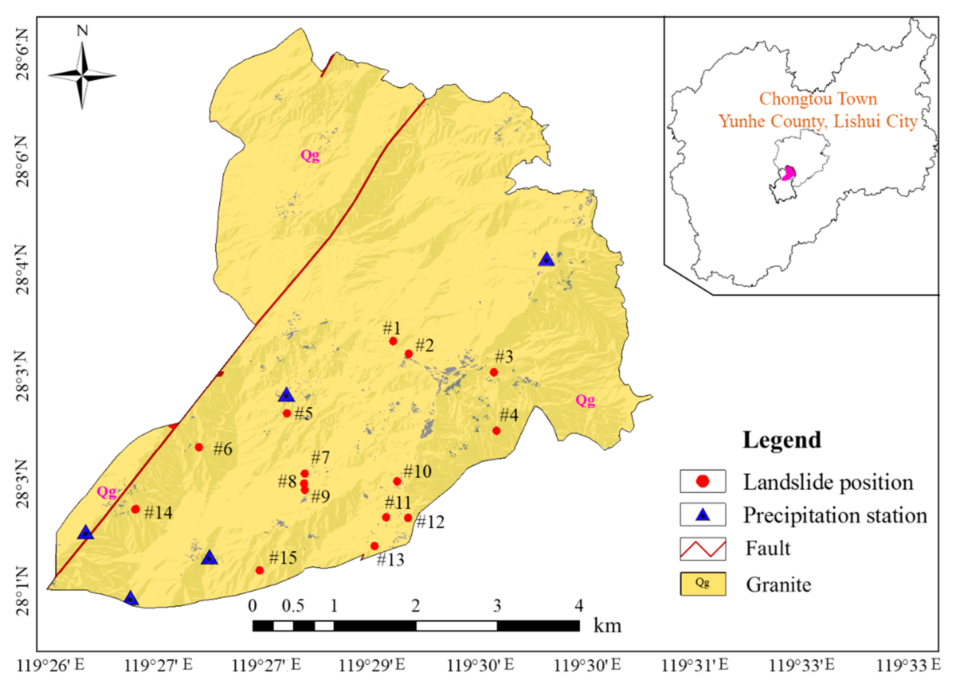
2. Study Area
2.1. Regional Geological Setting
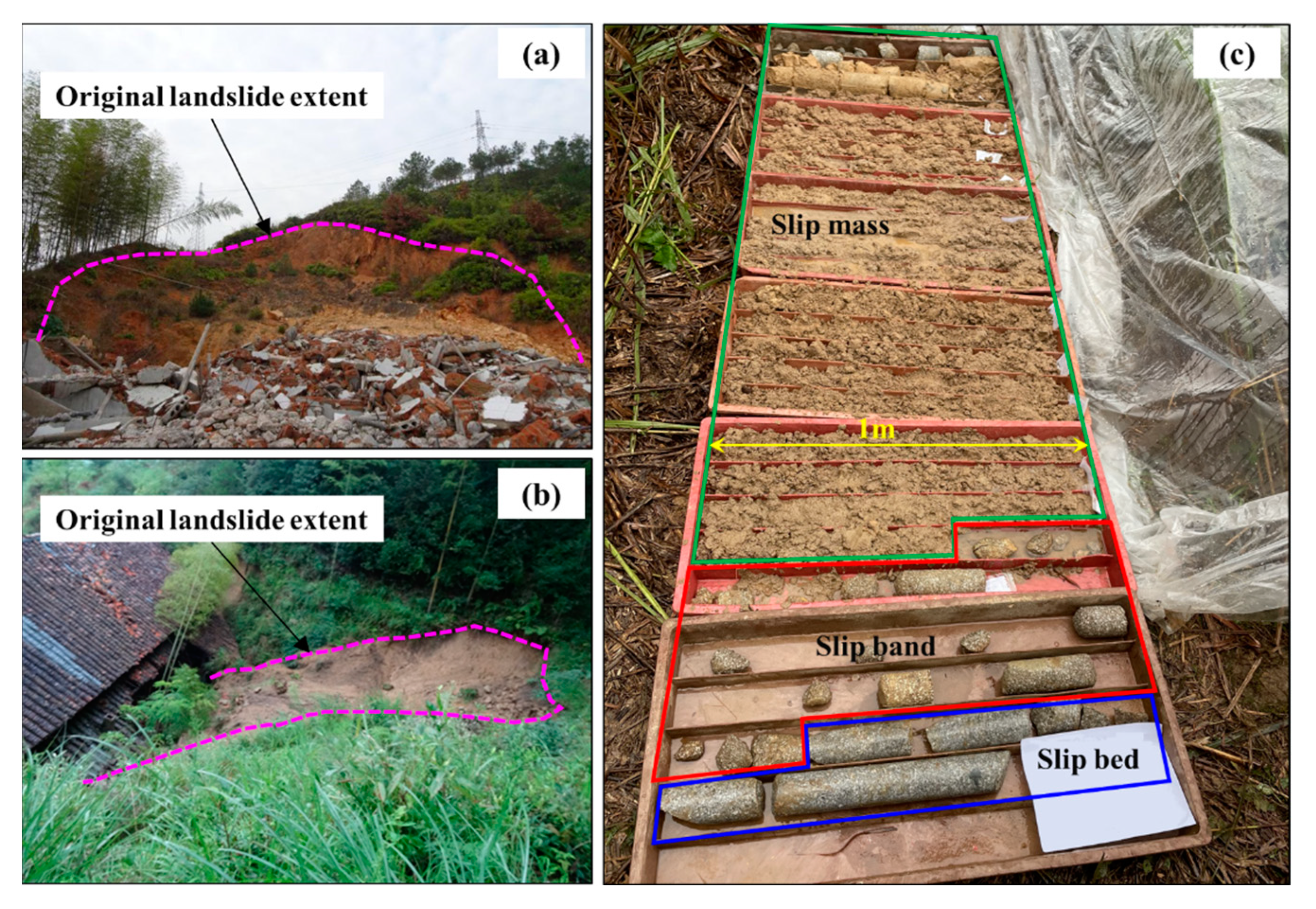
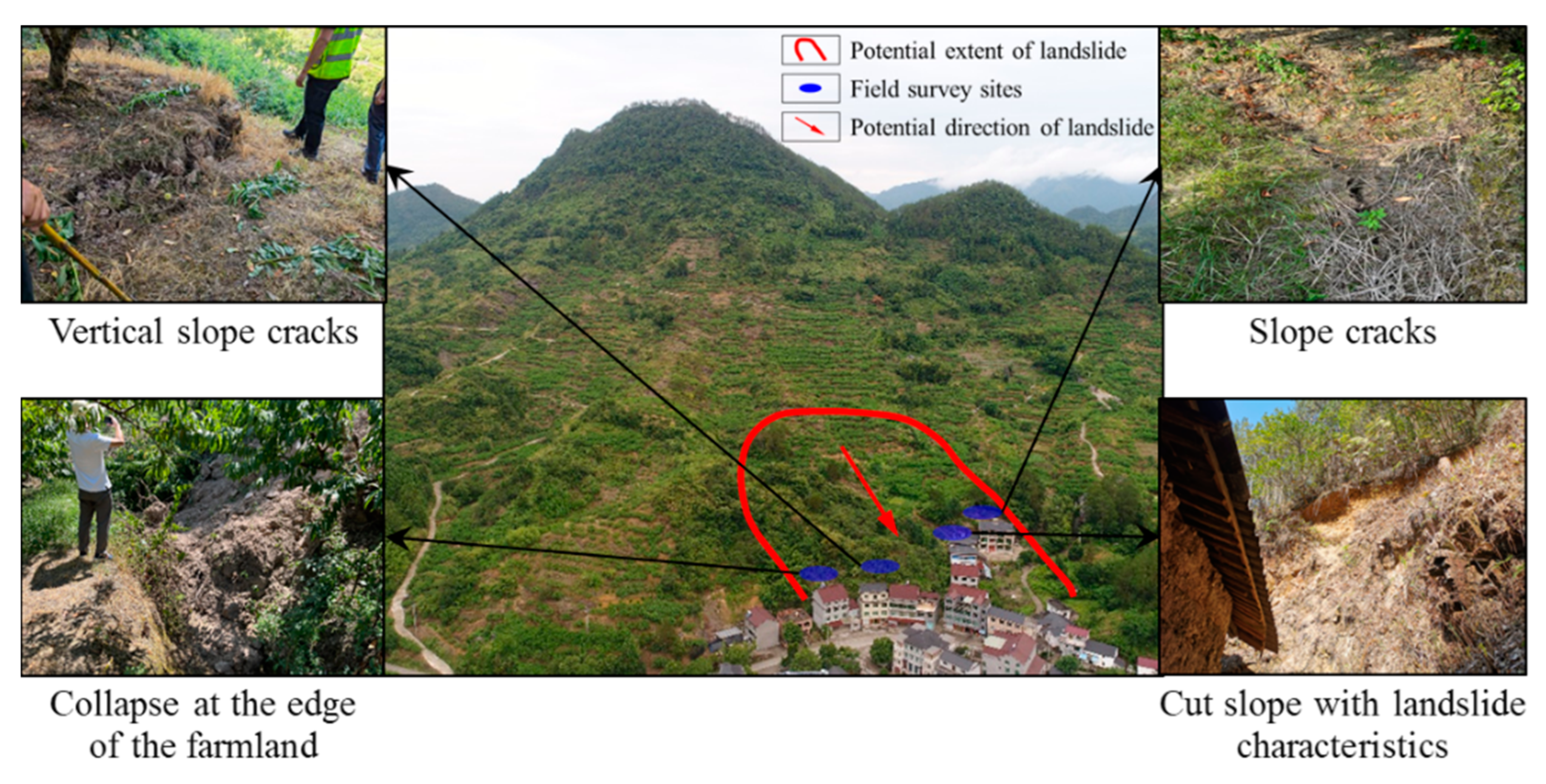
2.2. Characteristics of Historical Landslides
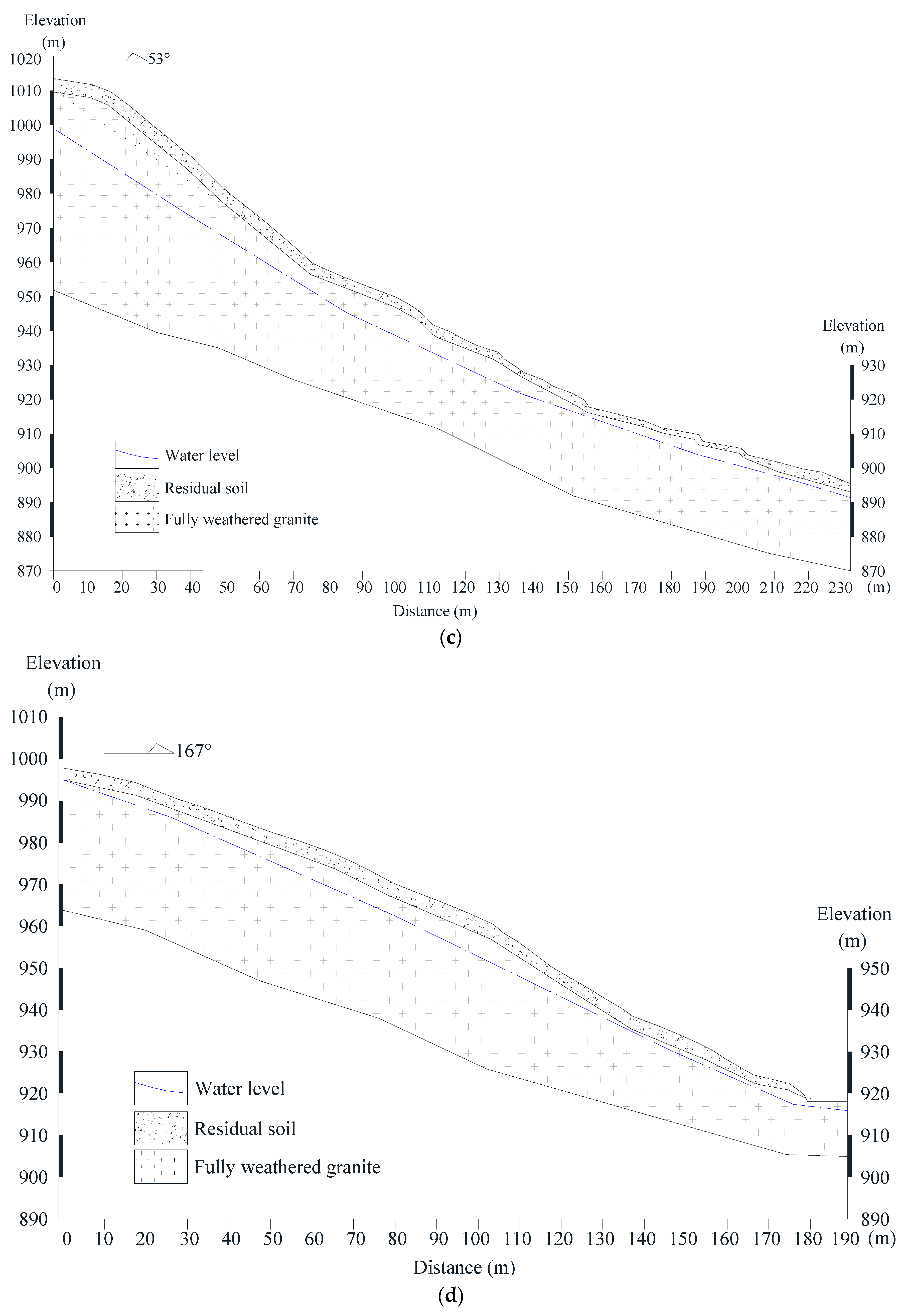
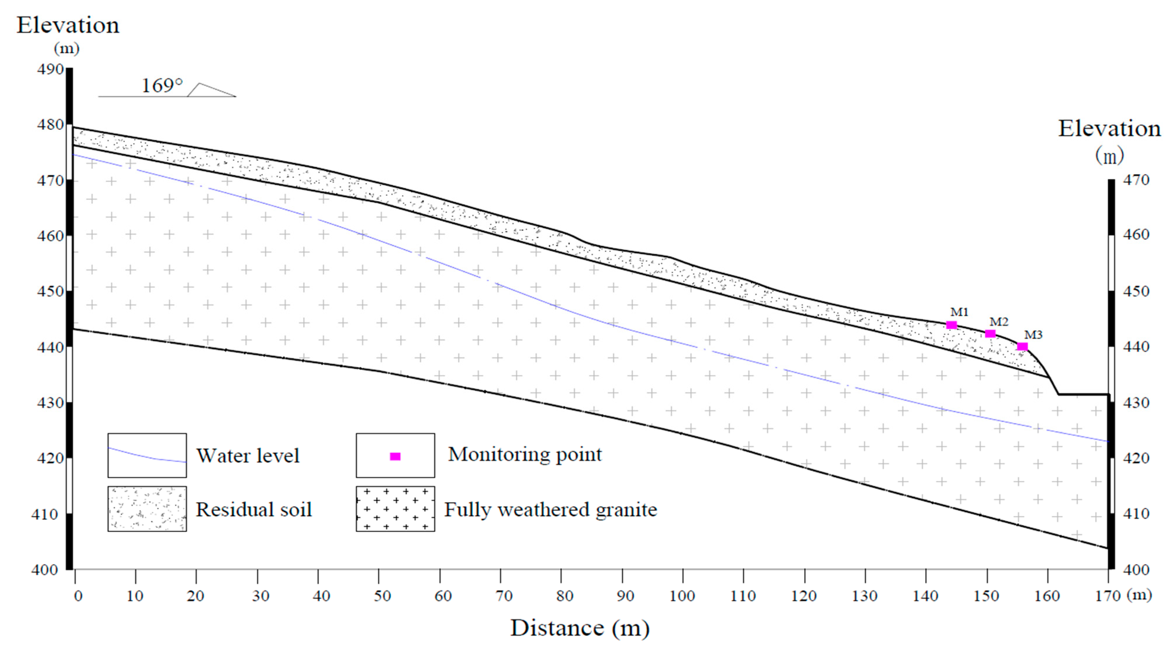
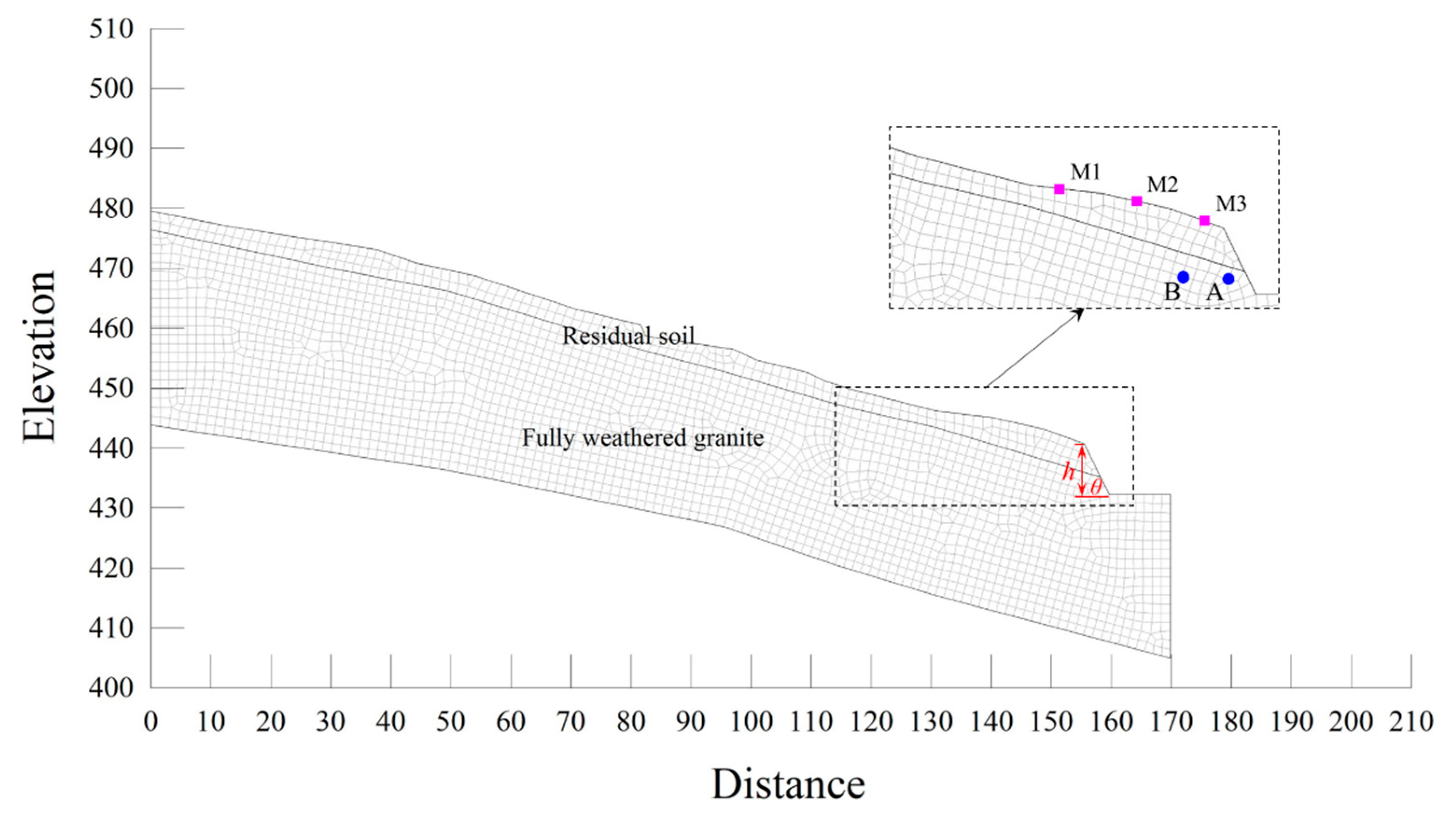
2.3. Engineering Conditions of a Typical Slope
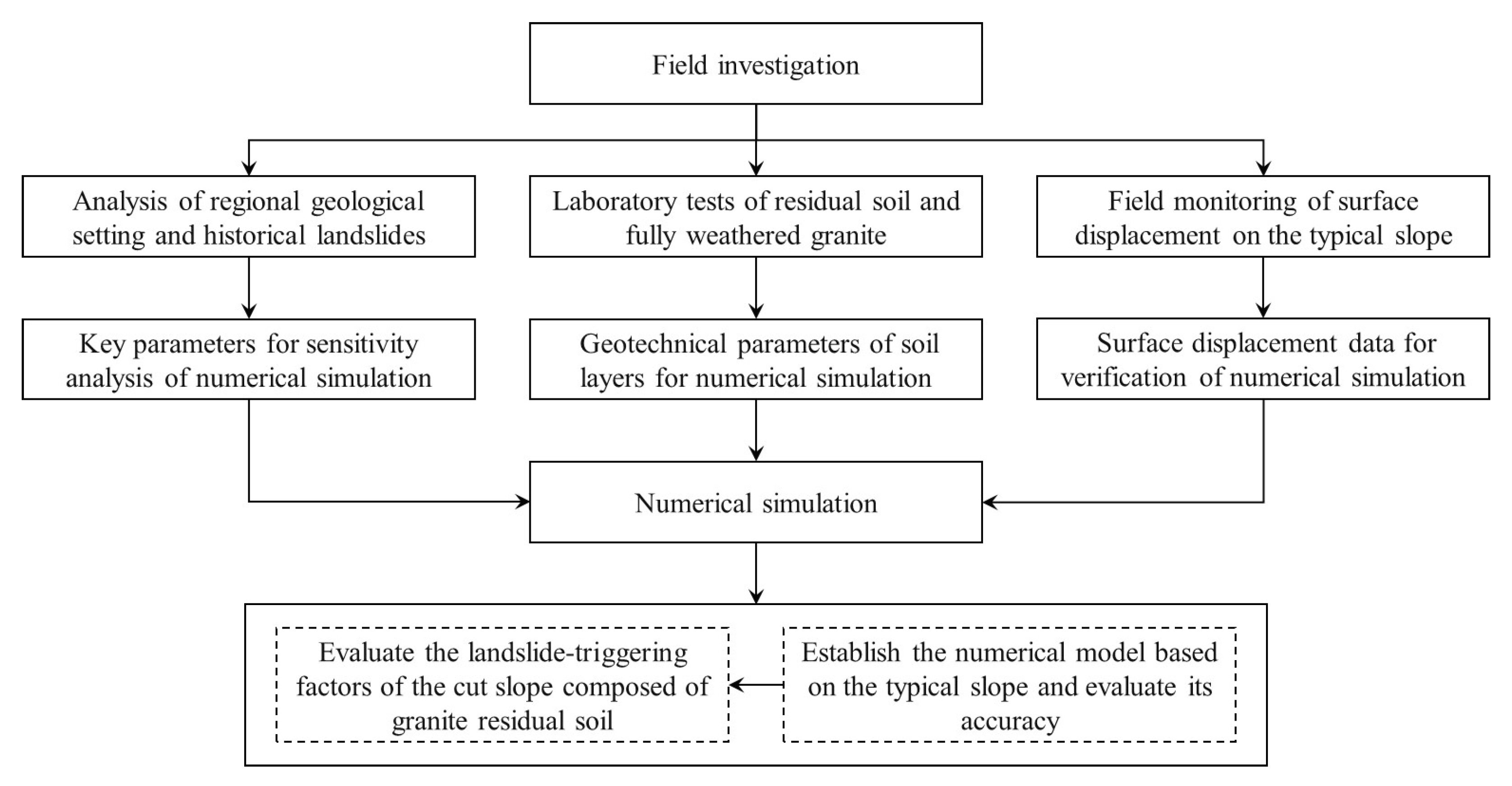
3. Materials and Methods
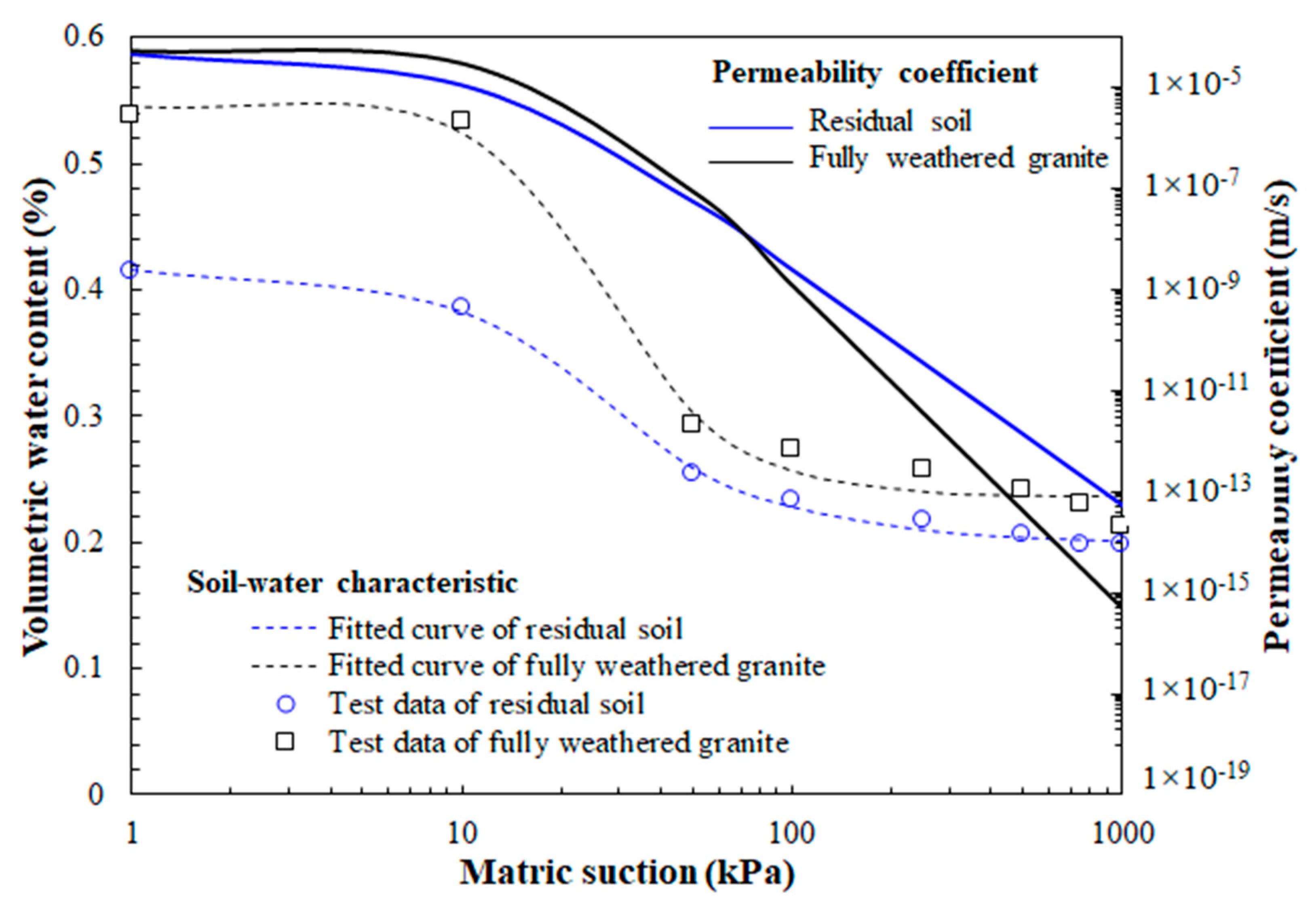
3.1. Laboratory Test
3.2. Field Test
3.3. Numerical Simulation
4. Results and Analysis
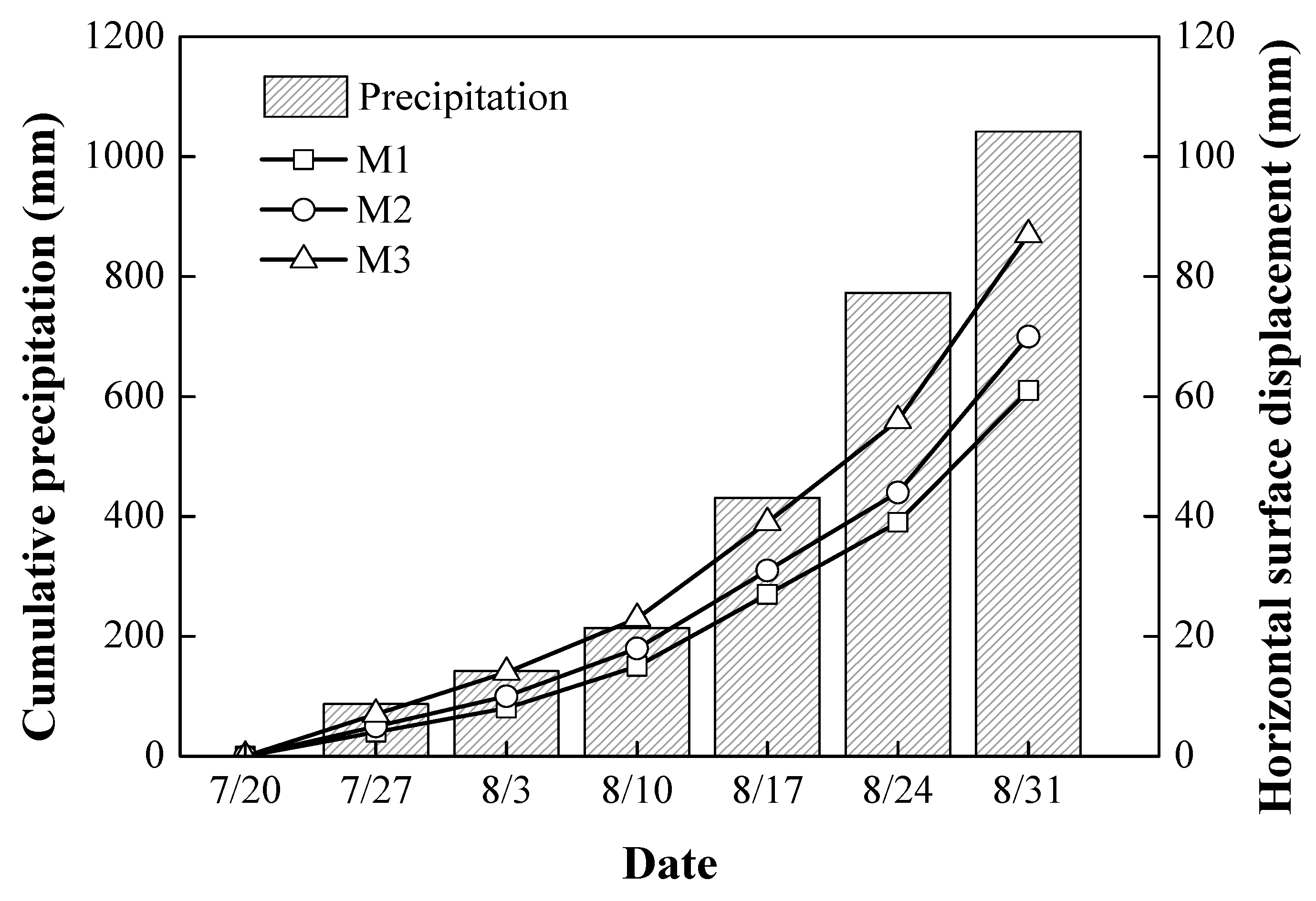
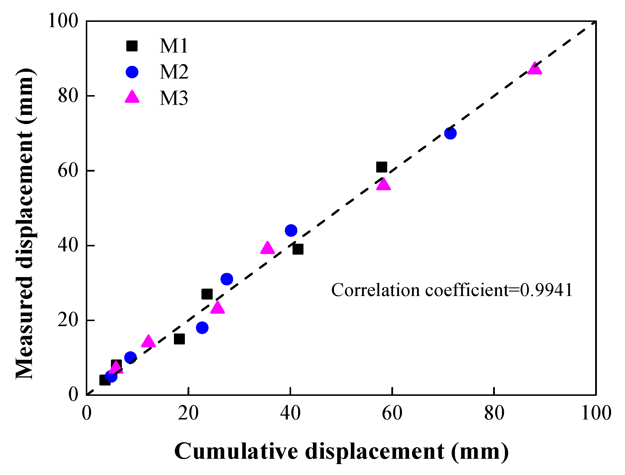
4.1. Comparison of The Horizontal Surface Displacement Derived from Field Tests and Numerical Simulations
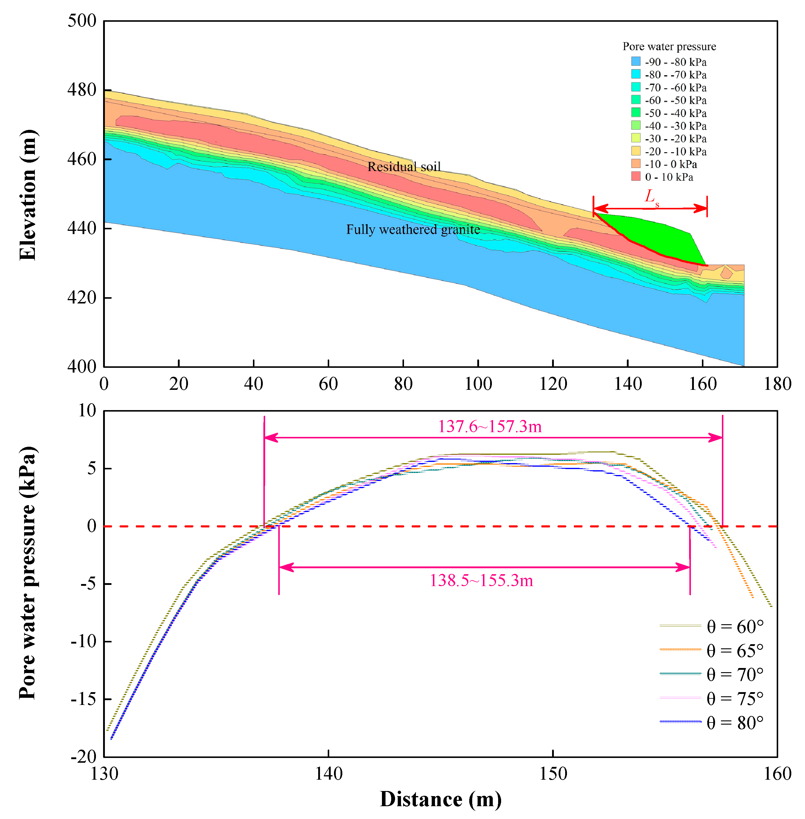
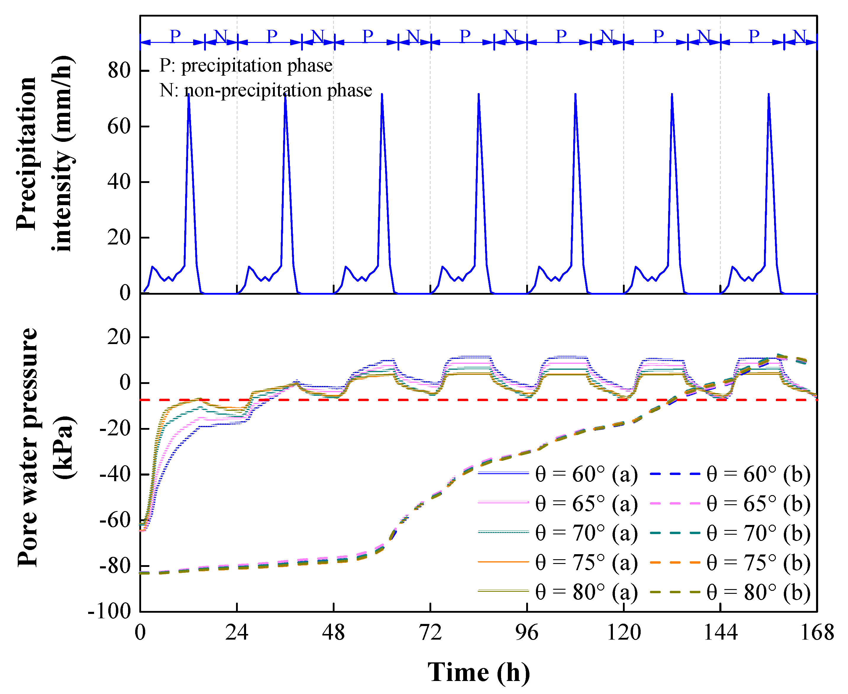
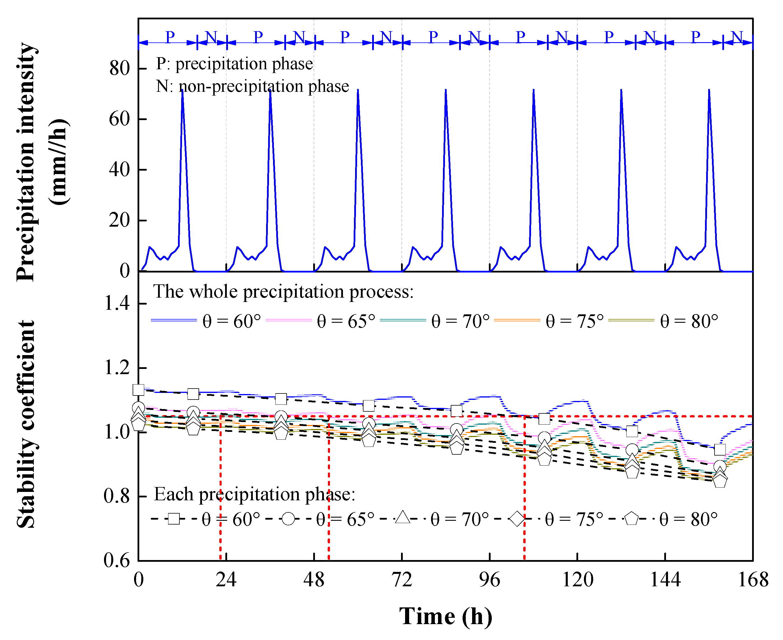
4.2. Effect of the Cut Slope’s Gradient on Slope Stability
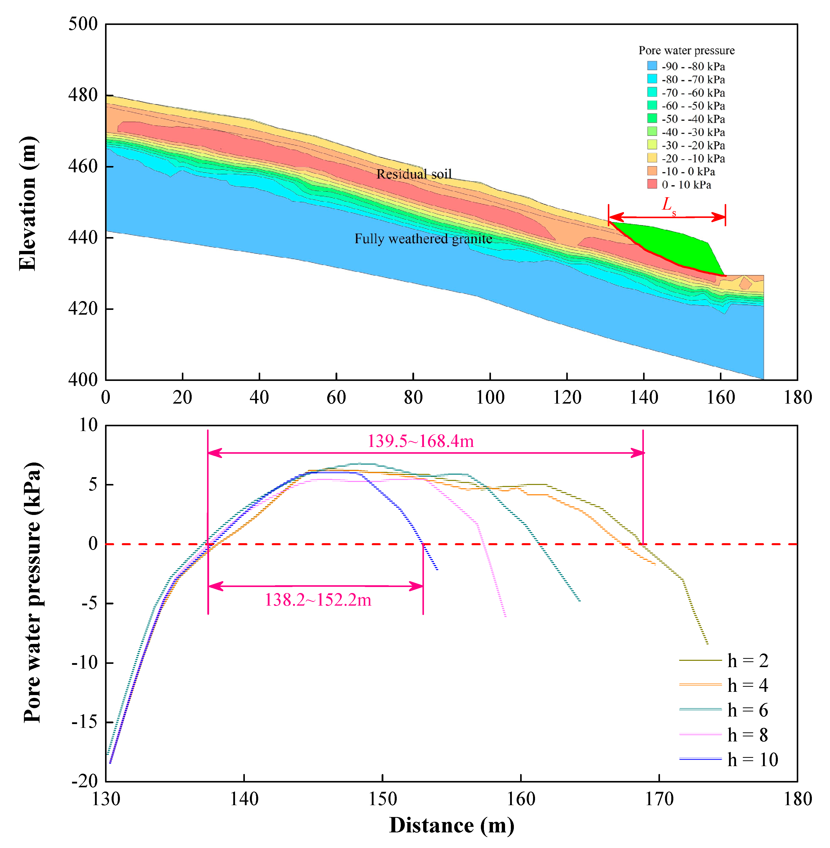
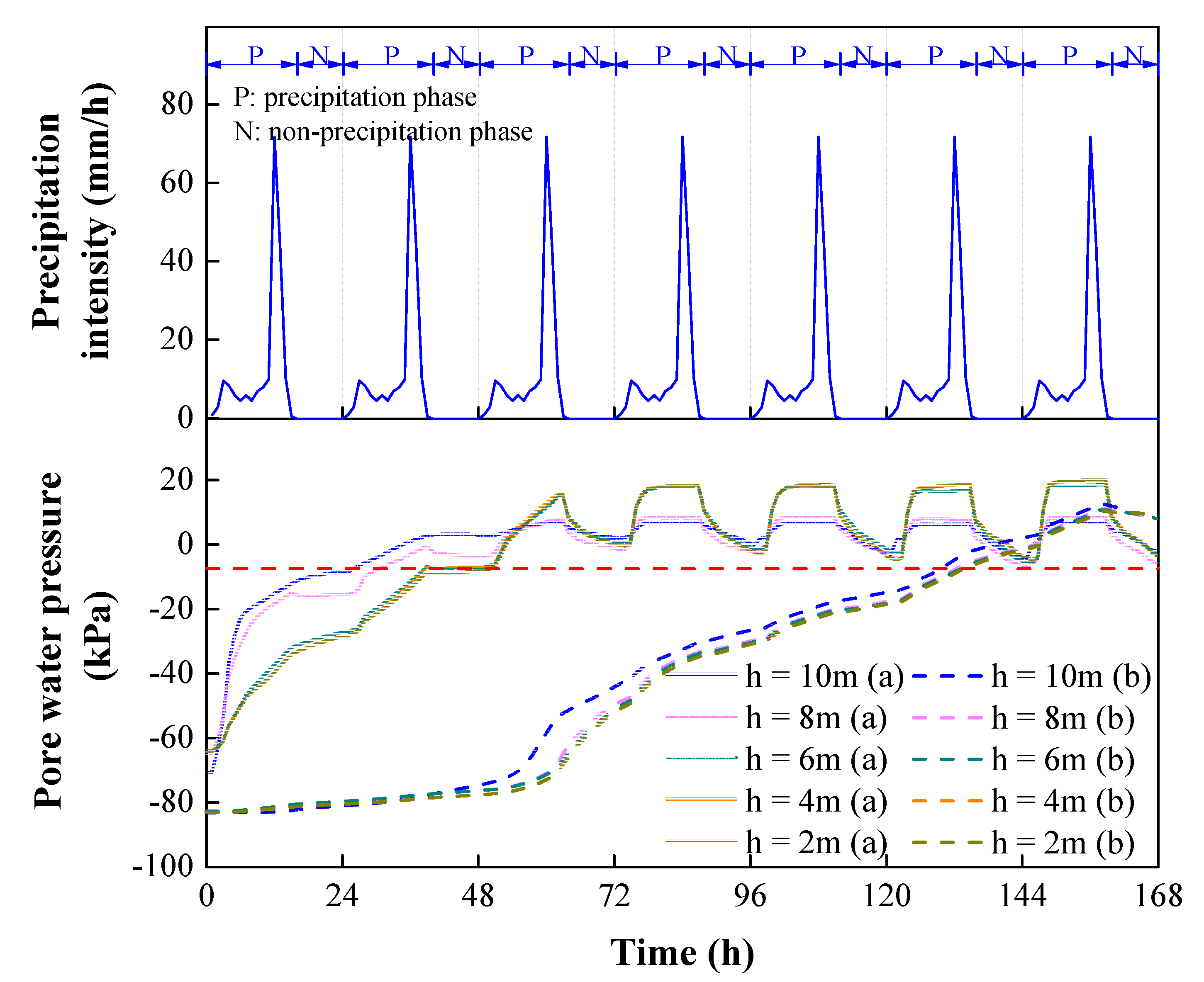
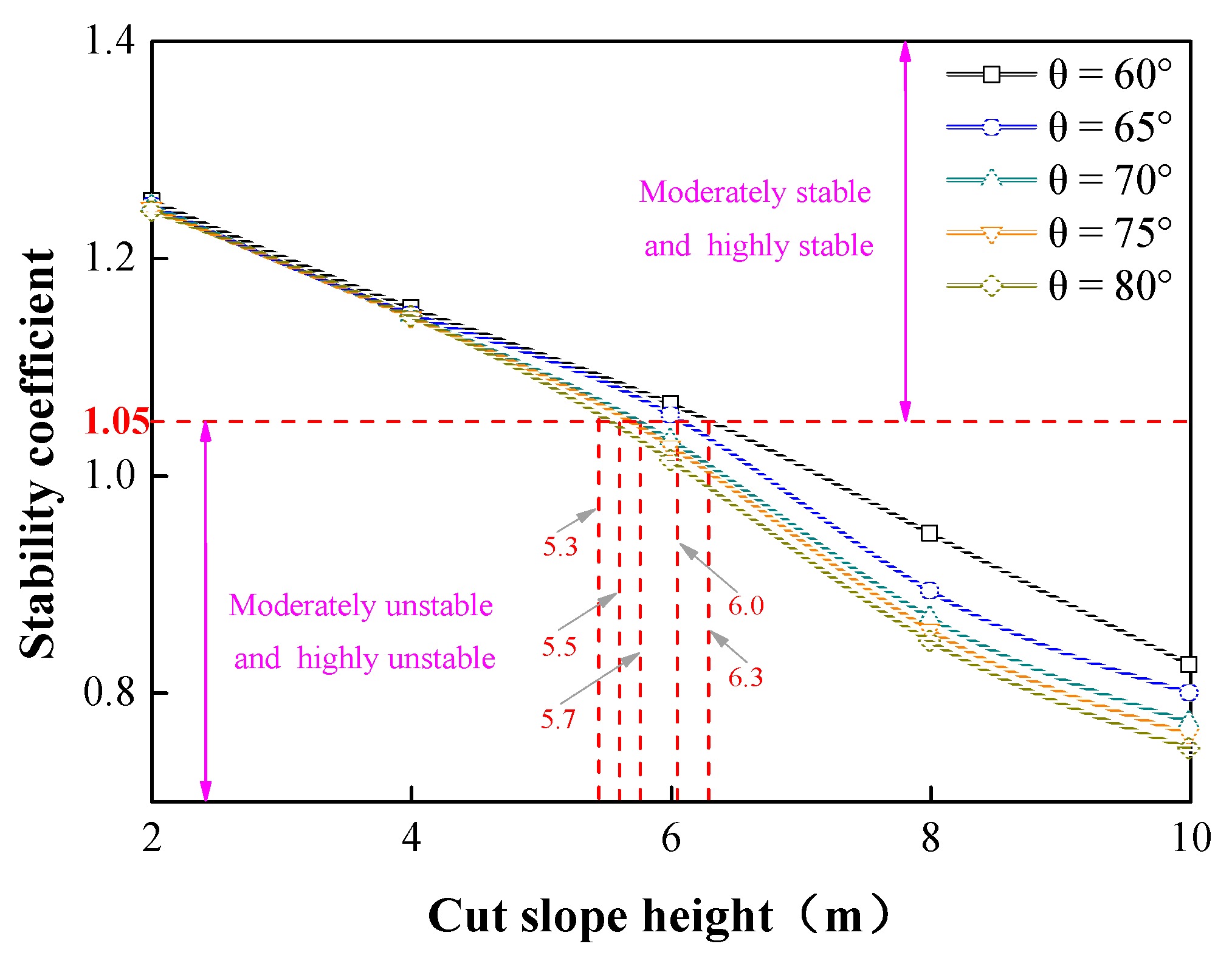
4.3. Effect of the Cut Slope’s Height on Slope Stability
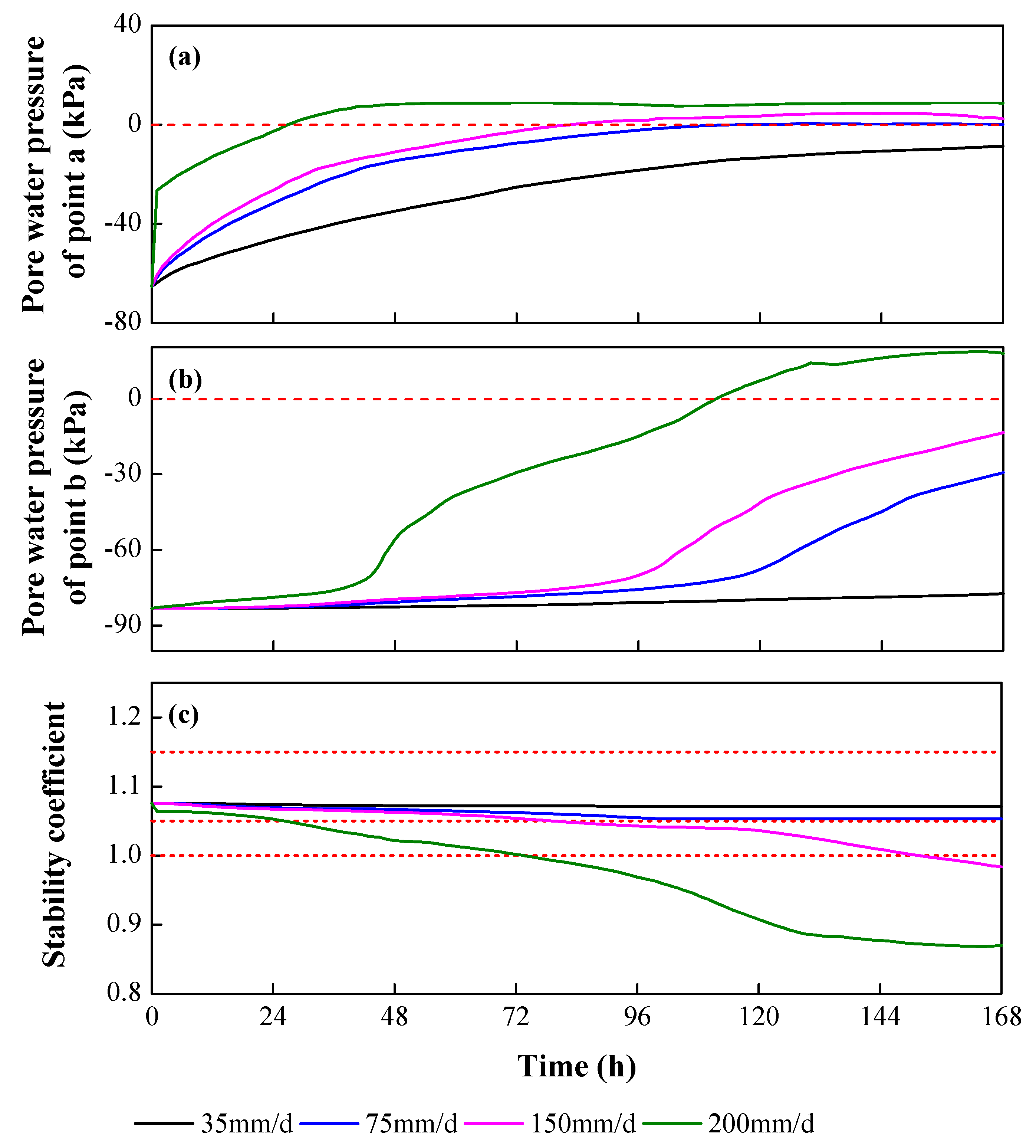
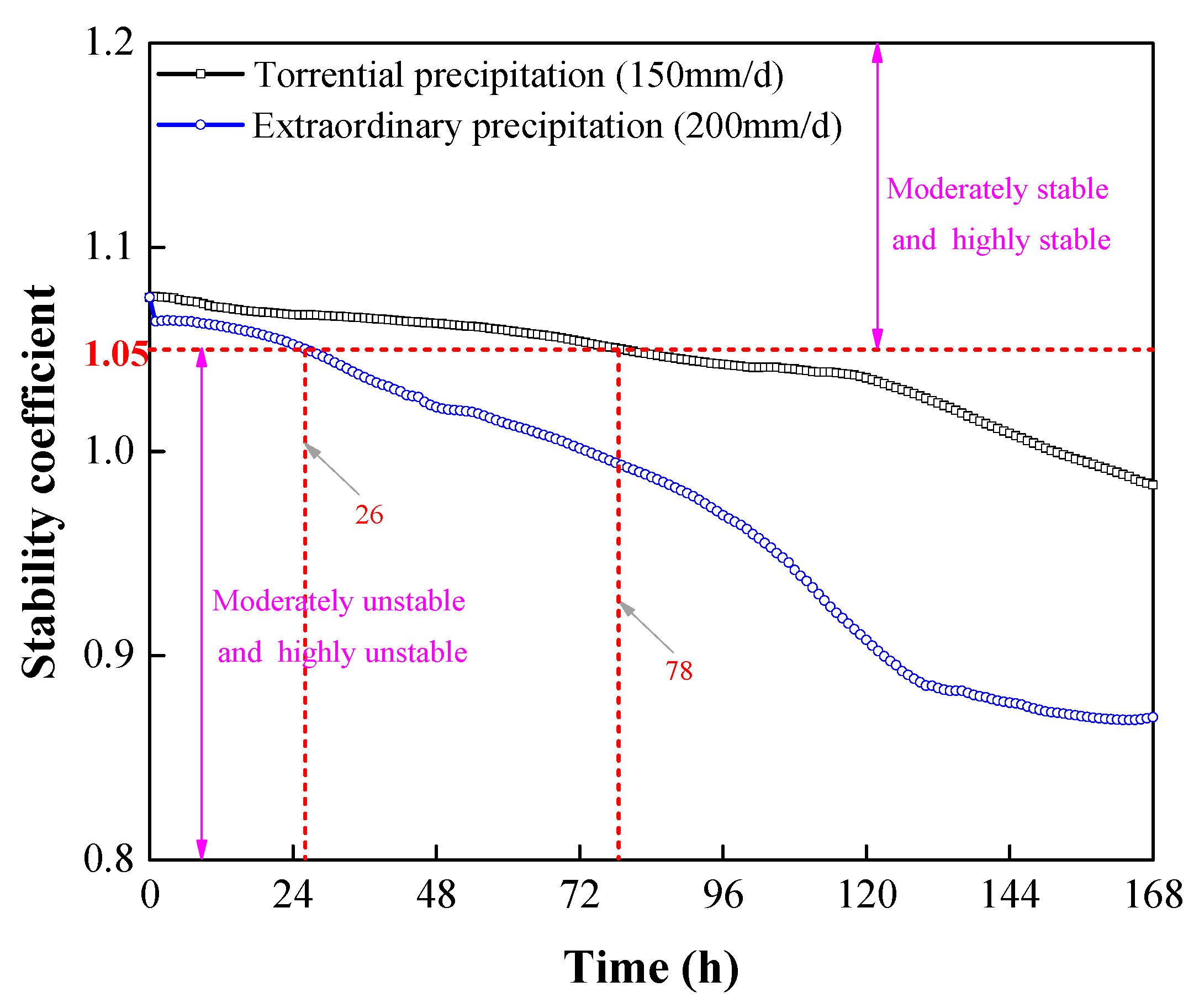
4.4. Effect of Precipitation Intensity on Slope Stability
5. Discussions of the Landslide Mechanism
- (a)
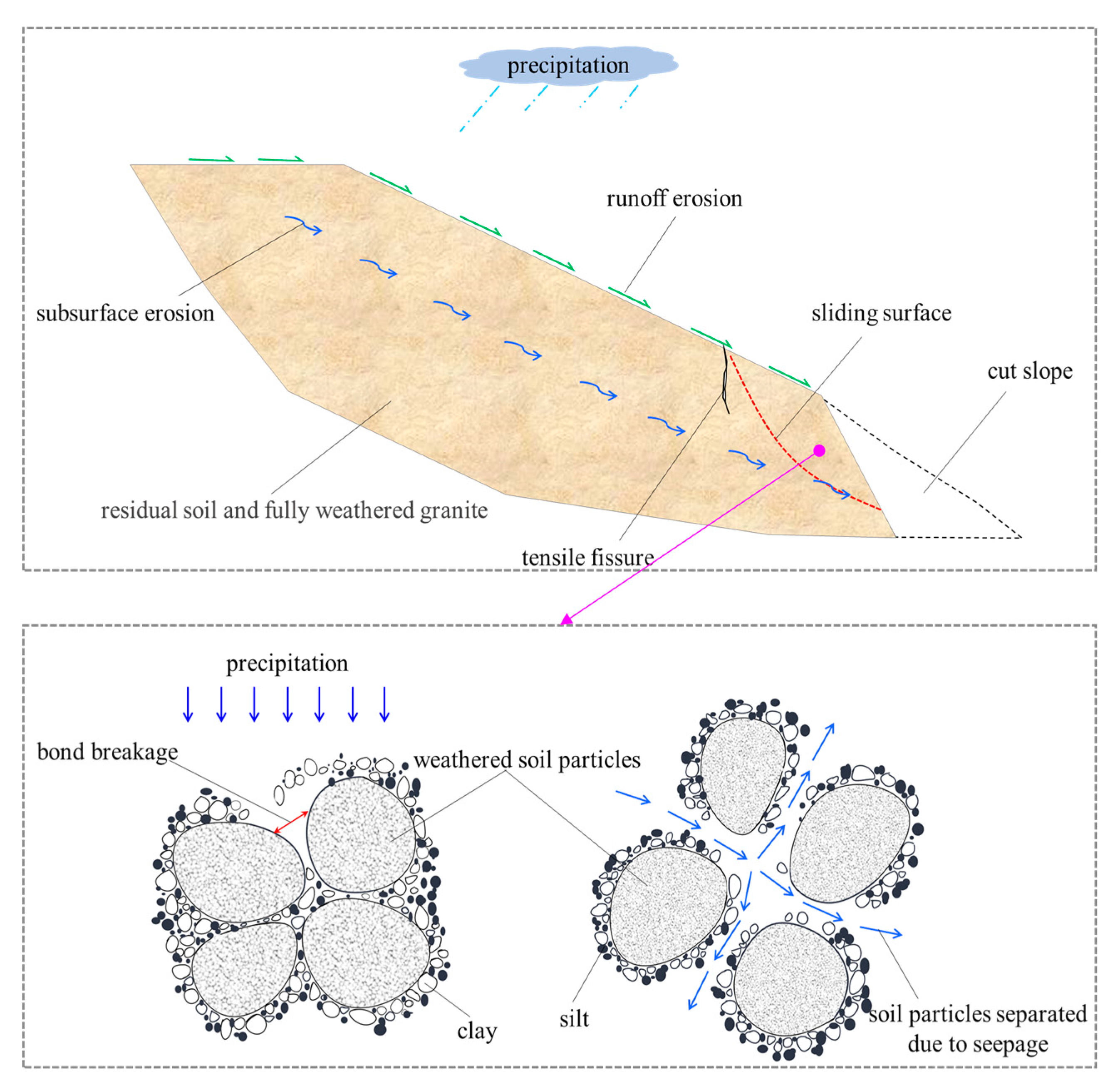
- Slope formation and evolution. A slope composed of granite residual soil was formed due to the climate, tectonics, and physical and mechanical properties of rock and soil. This soil is highly permeable, and its strength decreases rapidly as the water content increases.
- (b)
- Formation of unloading zone at slope foot. As shown in Figure 21, cutting the slope disrupted its mechanical equilibrium, forming an unloading zone. When the leading edge was cut, the stress of the unloading zone was released, and tensile fissures occurred. However, the slope remained stable.
- (c)
- Migration and loss of soil particles. The sand particles in the granite residual soil act as the skeleton and the clay and silt particles are attached to the skeleton, forming a combined structure [38] (Figure 21). Since the soil is a porous medium, the seepage field affects the soil skeleton due to rainwater infiltration. The change in the pore water pressure affects the effective stress on the soil skeleton; thus, the soil skeleton is deformed, and its strength is reduced.
- (d)
- Instability of cut slope. Due to rainfall infiltration, the pore water pressure in the unsaturated soil rises, the matric suction decreases, and the effective stress decreases. As a result, the shear strength of the soil and the slope stability decrease. In addition, tensile fissures occur at the top of the cut slope due to gravity and seepage, resulting in a landslide.

6. Engineering Implications

7. Conclusions
- (1)
- All historical landslides in the study area were small-scale and occurred at the foot of the slope. Different precipitation intensities and durations were observed 168 h before the landslide occurred. The intensity was general or heavy during this period but was the highest (heavy or torrential) on the date of the landslide.
- (2)
- The initial dry density, unit weight, shear strength, Poisson’s ratio, and saturated permeability coefficient of the residual soil and fully weathered granite were similar. The deformation modulus was 2.3 times larger for the fully weathered granite than the residual soil.
- (3)
- The field monitoring results showed that the deformation of the cut slope was positively correlated with the cumulative precipitation. The simulated and measured results were in good agreement, indicating that the proposed numerical model and parameters were accurate and reasonable.
- (4)
- As θ or h of the cut slope increased, the stability coefficient decreased, the response time of the pore water pressure at the observation points increased, and the horizontal length of the potential sliding surface decreased. The critical values of h were 5.3 m, 5.5 m, 5.7 m, 6.0 m, and 6.3 m at θ values of 60°, 65°, 70°, 75°, and 80°, respectively.
- (5)
- Long-term torrential precipitation or short-term extraordinary precipitation can trigger landslides of cut slopes. The stability coefficient was lower than 1.0 during precipitation events with durations of 26 h and 78 h, with a high likelihood of landslides of cut slopes.
- (6)
- The landslide causes of the cut slope composed of granite residual soil in southwest Zhejiang can be attributed to internal and external factors. The internal factors include the geotechnical soil properties and the slope’s structure, and the dominant external factor is precipitation. The formation of the slope and landslide includes four stages: slope evolution, formation of an unloading zone at the slope foot, migration and loss of soil particles, and instability of the cut slope.
Author Contributions
Funding
Institutional Review Board Statement
Informed Consent Statement
Data Availability Statement
Acknowledgments
Conflicts of Interest
References
- Bai, H.L.; Feng, W.K.; Li, S.Q.; Ye, L.Z.; Wu, Z.T.; Hu, R.; Dai, H.C.; Hu, P.Y.; Yi, X.Y.; Deng, P.C. Flow-slide characteristics and failure mechanism of shallow landslides in granite residual soil under heavy rainfall. J. Mt. Sci. 2022, 19, 1541–1557. [Google Scholar] [CrossRef]
- Zhang, C.Y.; Yin, Y.P.; Dai, Z.W.; Huang, B.; Zhang, Z.H.; Jiang, X.N.; Tan, W.J.; Wang, L.Q. Reactivation mechanism of a large-scale ancient landslide. Landslides 2021, 18, 397–407. [Google Scholar] [CrossRef]
- Prada-Sarmiento, L.F.; Cabrera, M.A.; Camacho, R.; Estrada, N.; Ramos-Cañón, A.M. The Mocoa Event on March 31 (2017): Analysis of a series of mass movements in a tropical environment of the Andean-Amazonian Piedmont. Landslides 2019, 16, 2459–2468. [Google Scholar] [CrossRef]
- Zhuang, J.Q.; Peng, J.B. A coupled slope cutting—A prolonged rainfall-induced loess landslide: A 17 October 2011 case study. Bull. Eng. Geol. Environ. 2014, 73, 997–1011. [Google Scholar] [CrossRef]
- Ouyang, C.J.; Zhao, W.; Xu, Q.; Peng, D.L.; Li, W.L.; Wang, D.P.; Zhou, S.; Hou, S.W. Failure mechanisms and characteristics of the 2016 catastrophic rockslide at Su village, Lishui, China. Landslides 2018, 15, 1391–1400. [Google Scholar] [CrossRef]
- Tu, X.B.; Kwong, A.K.L.; Dai, F.C.; Tham, L.G.; Min, H. Field monitoring of rainfall infiltration in a loess slope and analysis of failure mechanism of rainfall-induced landslides. Eng. Geol. 2009, 105, 134–150. [Google Scholar] [CrossRef]
- Xu, L.; Dai, F.C.; Tham, L.G.; Tu, X.B.; Min, H.; Zhou, Y.F.; Wu, C.X.; Xu, K. Field testing of irrigation effects on the stability of a cliff edge in loess, North-west China. Eng. Geol. 2011, 120, 10–17. [Google Scholar] [CrossRef]
- Zhang, W.C.; Wang, D. Stability analysis of cut slope with shear band propagation along a weak layer. Comput. Geotech. 2020, 125, 103676. [Google Scholar] [CrossRef]
- Qin, C.A.; Chen, G.Q.; Zhu, J.; Tang, P. A precursor of bedding rockslide: Rock spalling in the key block triggered by tensile cracks. Bull. Eng. Geol. Environ. 2020, 79, 2513–2528. [Google Scholar] [CrossRef]
- Awang, H.; Salmanfarsi, A.F.; Aminudin, M.S.; Ali, M.I. Stability of weathered cut slope by using kinematic analysis. In IOP Conference Series: Earth and Environmental Science; IOP Publishing: Bristol, UK, 2021; Volume 682, p. 012018. [Google Scholar]
- Panthee, S. Parametric evaluation of shear strength parameters on the stability of cut slope: A case study from Mahabaleshwar road section, India. J. Nepal Geol. Soc. 2016, 51, 73–76. [Google Scholar] [CrossRef]
- He, L.; Ren, Y.; Feng, Z.X.; Han, Z.W. Numerical simulation and design optimization Research of slope ratio and platforms influence on a high rock cut slope engineering stability. In Advanced Materials Research; Trans Tech Publications Ltd.: Stafa-Zurich, Switzerland, 2015; Volume 1065, pp. 151–158. [Google Scholar]
- Cao, C.S.; Wu, S.R.; Pan, M.; Liang, C.Y. Mechanism research on artificial slope cutting-induced loess landslide. Rock Soil Mech. 2016, 37, 1049–1060. [Google Scholar]
- Mei, Y.; Zhou, D.B.; Hu, C.M.; Wang, X.Y.; Zhang, Y.H.; Xiao, N.; Shi, W.Y. Study on Deformation Characteristics of Loess Ultrahigh-Fill Slope Based on Large-Scale Undisturbed Soil Centrifugal Model Tests. Front. Earth Sci. 2022, 10, 848542. [Google Scholar] [CrossRef]
- Sun, P.; Wang, H.J.; Wang, G.; Li, R.J.; Zhang, Z.; Huo, X.T. Field model experiments and numerical analysis of rainfall-induced shallow loess landslides. Eng. Geol. 2021, 295, 106411. [Google Scholar] [CrossRef]
- Postill, H.; Helm, P.R.; Dixon, N.; Glendinning, S.; Smethurst, J.A.; Rouainia, M.; Briggs, K.M.; Blake, A.P. Forecasting the long-term deterioration of a cut slope in high-plasticity clay using a numerical model. Eng. Geol. 2021, 280, 105912. [Google Scholar] [CrossRef]
- Wang, L.; Li, G.; Chen, Y.; Tan, J.M.; Wang, S.M.; Guo, F. Field model test on failure mechanism of artificial cut-slope rainfall in Southern Jiangxi. Rock Soil Mech. 2021, 42, 846–854. [Google Scholar]
- Jin, H.H.; Wang, L.F.; Zhang, X.X. Analysis of the stability evolution process and prediction method of high cutting slope under rainfall cycle condition. J. Civ. Environ. Eng. 2021, 43, 12–23. [Google Scholar]
- Pradhan, S.P.; Siddique, T. Stability assessment of landslide-prone road cut rock slopes in Himalayan terrain: A finite element method based approach. J. Rock Mech. Geotech. Eng. 2020, 12, 59–73. [Google Scholar] [CrossRef]
- Luo, Y.; Xiao, M.L. Stability analysis for pre-reinforced piles within high cutting slope. Eur. J. Environ. Civ. Eng. 2020, 1–13. [Google Scholar] [CrossRef]
- Katz, O.; Reichenbach, P.; Guzzetti, F. Rock fall hazard along the railway corridor to Jerusalem, Israel, in the Soreq and Refaim valleys. Nat. Hazards 2011, 56, 649–665. [Google Scholar] [CrossRef]
- Chirico, G.B.; Borga, M.; Tarolli, P.; Rigon, R.; Preti, F. Role of vegetation on slope stability under transient unsaturated conditions. Procedia Environ. Sci. 2013, 19, 932–941. [Google Scholar] [CrossRef]
- Chen, F.; Xu, Y.; Wang, C.; Mao, J. Effects of concrete content on seed germination and seedling establishment in vegetation concrete matrix in slope restoration. Ecol. Eng. 2013, 58, 99–104. [Google Scholar] [CrossRef]
- Normaniza, O.; Faisal, H.A.; Barakbah, S.S. Engineering properties of Leucaena leucocephala for prevention of slope failure. Ecol. Eng. 2008, 32, 215–221. [Google Scholar] [CrossRef]
- Ai, Y.; Chen, Z.; Guo, P.; Zeng, L.; Liu, H.; Da, Z.; Li, W. Fractal characteristics of synthetic soil for cut slope revegetation in the Purple soil area of China. Can. J. Soil Sci. 2012, 92, 277–284. [Google Scholar] [CrossRef]
- Chen, Z.; Wang, K.; Ai, Y.W.; Li, W.; Gao, H.; Fang, C. The effects of railway transportation on the enrichment of heavy metals in the artificial soil on railway cut slopes. Environ. Monit. Assess. 2014, 186, 1039–1049. [Google Scholar] [CrossRef] [PubMed]
- Lee, D.H.; Yang, Y.E.; Lin, H.M. Assessing slope protection methods for weak rock slopes in Southwestern Taiwan. Eng. Geol. 2007, 91, 100–116. [Google Scholar] [CrossRef]
- GB/T 50123–2019; Ministry of Housing and Urban Rural Development of the People’s Republic of China (MHURD-PRC) “Chinese Standard for Geotechnical Testing Method”. China Planning Press: Beijing, China, 2019.
- Van Genuchten, M.T. A closed-form equation for predicting the hydraulic conductivity of unsaturated soils. Soil Sci. Soc. Am. J. 1980, 44, 892–898. [Google Scholar] [CrossRef]
- Gao, J.J.; Xu, H.; Qian, J.W.; Gong, Y.F.; Zhan, L.T.; Chen, P. Settlement behavior of soft subgrade reinforced by geogrid-encased stone column and geocell-embedded sand cushion: A numerical analysis. Adv. Civ. Eng. 2020, 2020, 8874520. [Google Scholar] [CrossRef]
- Vanapalli, S.K.; Fredlund, D.G.; Pufahl, D.E.; Clifton, A.W. Model for the prediction of shear strength with respect to soil suction. Can. Geotech. J. 1996, 33, 379–392. [Google Scholar] [CrossRef]
- GB/T 32864–2016; Code for Geological Investigation of Landslide Prevention. Standards Press of China: Beijing, China, 2016.
- Hou, T.S.; Xu, G.L.; Zhang, D.Q.; Liu, H.Y. Stability analysis of Gongjiacun landslide in the three Gorges Reservoir area under the action of reservoir water level fluctuation and rainfall. Nat. Hazards 2022, 114, 1647–1683. [Google Scholar] [CrossRef]
- Singh, V.P.; Joseph, E.S. Kinematic-wave model for soil-moisture movement with plant-root extraction. Irrig. Sci. 1994, 14, 189–198. [Google Scholar] [CrossRef]
- Wei, X.S.; Fan, W.; Chai, X.Q.; Cao, Y.B.; Nan, Y.L. Field and numerical investigations on triggering mechanism in typical rainfall-induced shallow landslides: A case study in the Ren River catchment, China. Nat. Hazards 2020, 103, 2145–2170. [Google Scholar] [CrossRef]
- Wang, D.Y.; Zeng, Q.J.; Wang, J.; Zhou, M. Effect of Dry-Wet Cycle on Stability of Granite Residual Soil Slope. In IOP Conference Series: Earth and Environmental Science; IOP Publishing: Bristol, UK, 2020; Volume 526, p. 012046. [Google Scholar]
- Zhang, S.; Tang, H.M. Experimental study of disintegration mechanism for unsaturated granite residual soil. Rock Soil Mech. 2013, 34, 1668–1674. [Google Scholar]
- Liu, X.; Zhang, X.; Kong, L.; Li, X.; Wang, G. Effect of cementation on the small-strain stiffness of granite residual soil. Soils Found. 2021, 61, 520–532. [Google Scholar] [CrossRef]


| Number | Date | Landslide Volume (m3) | Height of the Natural Slope (h) (m) | Gradient of the Natural Slope (α) (°) | Height of the Cut Slope (h) (m) | Gradient of the Cut Slope (θ) (°) | Thickness of Residual Soil (m) | Thickness of Fully Weathered Granite (m) |
|---|---|---|---|---|---|---|---|---|
| #1 | 1 August 2011 | 300 | 65 | 15~25 | 2~8 | 65~70 | 2~3 | 20~25 |
| #2 | 1 June 2014 | 2400 | 83 | 15~25 | 4~8 | 60~70 | 3~4 | 20~25 |
| #3 | 14 June 2014 | 9500 | 96 | 25~35 | 4~8 | 65~80 | 3~5 | 25~30 |
| #4 | 6 July 2010 | 200 | 112 | 25~35 | 6~8 | 65~70 | 2~3 | 15~20 |
| #5 | 13 September 2015 | 1200 | 79 | 25~35 | 3~10 | 60~70 | 2~3 | 20~25 |
| #6 | 9 July 2020 | 1350 | 91 | 25~35 | 6~10 | 60~75 | 3~4 | 20~25 |
| #7 | 1 May 2015 | 800 | 116 | 25~35 | 5~8 | 65~80 | 2~3 | 20~25 |
| #8 | 4 July 1997 | 7400 | 89 | 15~25 | 5~10 | 65~80 | 3~5 | 25~30 |
| #9 | 8 July 2020 | 320 | 105 | 25~35 | 2~6 | 65~75 | 2~3 | 15~20 |
| #10 | 11 October 2008 | 450 | 58 | 15~25 | 2~6 | 60~75 | 2~3 | 15~20 |
| #11 | 21 September 2015 | 500 | 95 | 25~35 | 5~10 | 65~80 | 2~3 | 15~20 |
| #12 | 17 April 2017 | 300 | 82 | 15~25 | 2~8 | 65~70 | 2~3 | 15~20 |
| #13 | 1 August 2009 | 1350 | 61 | 25~35 | 2~8 | 60~70 | 3~4 | 20~25 |
| #14 | 23 July 2010 | 800 | 73 | 15~25 | 2~8 | 60~75 | 2~3 | 20~25 |
| #15 | 7 October 2013 | 4400 | 69 | 15~25 | 3~9 | 65~80 | 3~5 | 25~30 |
| Parameters | Value |
|---|---|
| Height of the natural slope (H) (m) | 75 |
| Gradient of the natural slope (α) (°) | 27 |
| Height of the cut slope (h) (m) | 8 |
| Gradient of the cut slope (θ) (°) | 65 |
| Thickness of residual soil (m) | 2.8 |
| Thickness of fully weathered granite (m) | 30 |
| Soil Layer | Initial Dry Density (g/cm3) | Unit Weight (kN/m3) | Cohesion (kPa) | Internal Friction Angle (°) | Saturated Permeability Coefficient (m/s) | Poisson’s Ratio | Deformation Modulus (MPa) |
|---|---|---|---|---|---|---|---|
| Residual soil | 1.34 | 18.6 | 14.3 | 12.1 | 5.3 × 10 −5 | 0.32 | 13.7 |
| Fully weathered granite | 1.42 | 19.6 | 15.4 | 18.7 | 5.6 × 10 −5 | 0.28 | 31.5 |
| Soil Layer | θr | θs | α | m | R2 |
|---|---|---|---|---|---|
| Residual soil | 0.1992 | 0.4169 | 0.0629 | 0.5184 | 0.9975 |
| Fully weathered granite | 0.2357 | 0.5454 | 0.0460 | 0.6381 | 0.9889 |
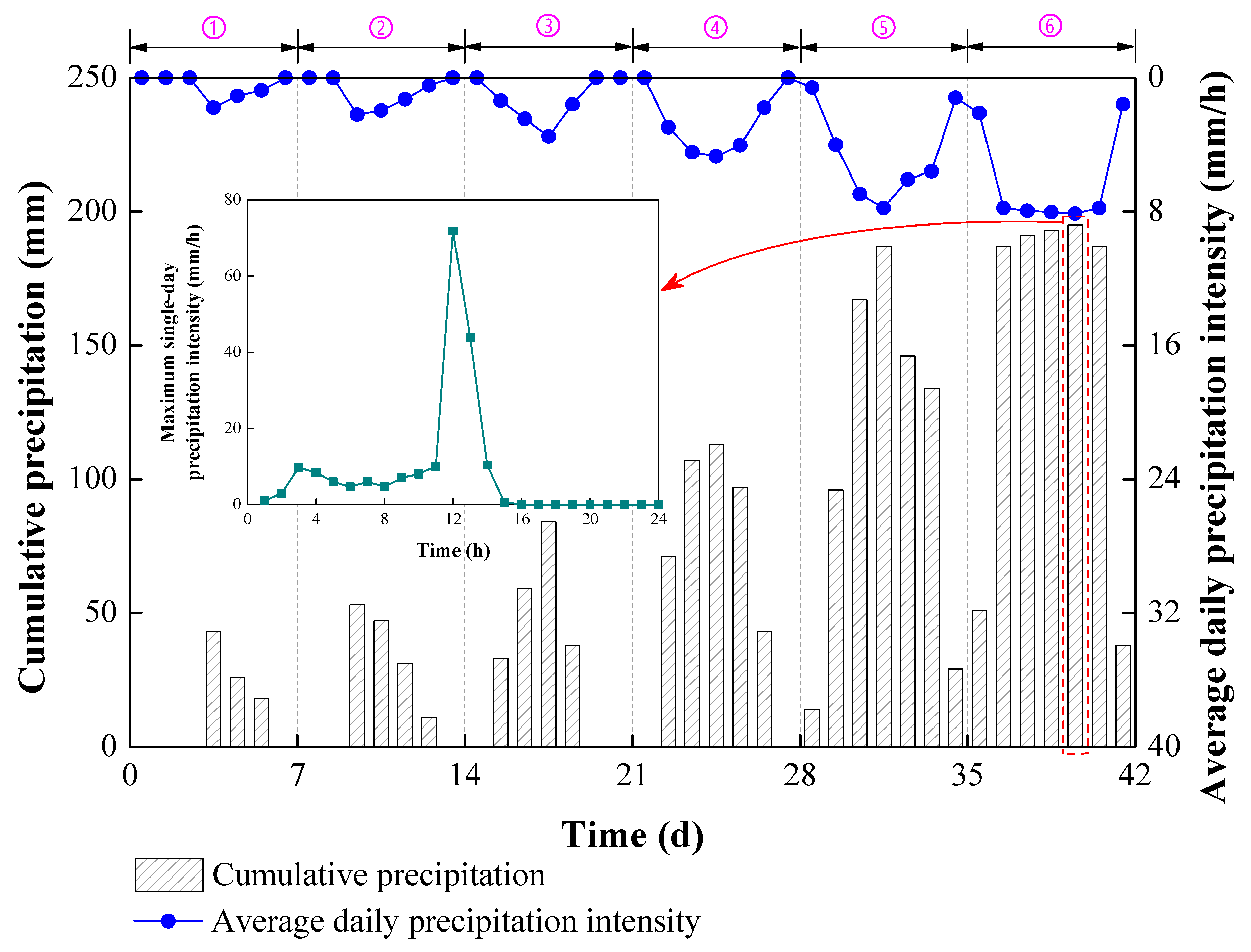
| Monitoring Stage | Date | Duration (d) | Accumulated Precipitation (mm) | Maximum Daily Precipitation (mm) | Date of the Maximum Daily Precipitation |
|---|---|---|---|---|---|
| ① | 20 July 2022~26 July 2022 | 7 | 87 | 43.1 | 7/23 |
| ② | 27 July 2022~2 August 2022 | 7 | 142 | 53.4 | 7/29 |
| ③ | 3 August 2022~9 August 2022 | 7 | 214 | 84.3 | 8/6 |
| ④ | 10 August 2022~16 August 2022 | 7 | 431 | 112.6 | 8/13 |
| ⑤ | 17 August 2022~23 August 2022 | 7 | 773 | 187.1 | 8/20 |
| ⑥ | 24 August 2022~30 August 2022 | 7 | 1042 | 195.7 | 8/28 |
| Case Number | Gradient of the Cut Slope (θ) (°) | Height of the Cut Slope (h) (m) | Precipitation Intensity | Precipitation Duration |
|---|---|---|---|---|
| H-1 | 65 | 2 | Monitoring data of precipitation on August 28 | 7 d |
| H-2 | 4 | |||
| H-3 | 6 | |||
| H-4 | 8 | |||
| H-5 | 10 | |||
| G-1 | 60 | 8 | Monitoring data of precipitation on August 28 | 7 d |
| G-2 | 65 | |||
| G-3 | 70 | |||
| G-4 | 75 | |||
| G-5 | 80 | |||
| P-1 | 65 | 8 | 35 mm/d | 7 d |
| P-2 | 75 mm/d | |||
| P-3 | 150 mm/d | |||
| P-4 | 200 mm/d |
| Stability Coefficient | Fs < 1.00 | 1.00 ≤ Fs < 1.05 | 1.05 ≤ Fs < 1.15 | Fs ≥ 1.15 |
|---|---|---|---|---|
| State | Highly unstable | Moderately unstable | Moderately stable | Highly stable |
Disclaimer/Publisher’s Note: The statements, opinions and data contained in all publications are solely those of the individual author(s) and contributor(s) and not of MDPI and/or the editor(s). MDPI and/or the editor(s) disclaim responsibility for any injury to people or property resulting from any ideas, methods, instructions or products referred to in the content. |
© 2023 by the authors. Licensee MDPI, Basel, Switzerland. This article is an open access article distributed under the terms and conditions of the Creative Commons Attribution (CC BY) license (https://creativecommons.org/licenses/by/4.0/).
Share and Cite
Yan, T.; Xiong, J.; Ye, L.; Gao, J.; Xu, H. Field Investigation and Finite Element Analysis of Landslide-Triggering Factors of a Cut Slope Composed of Granite Residual Soil: A Case Study of Chongtou Town, Lishui City, China. Sustainability 2023, 15, 6999. https://doi.org/10.3390/su15086999
Yan T, Xiong J, Ye L, Gao J, Xu H. Field Investigation and Finite Element Analysis of Landslide-Triggering Factors of a Cut Slope Composed of Granite Residual Soil: A Case Study of Chongtou Town, Lishui City, China. Sustainability. 2023; 15(8):6999. https://doi.org/10.3390/su15086999
Chicago/Turabian StyleYan, Tiesheng, Jun Xiong, Longjian Ye, Jiajun Gao, and Hui Xu. 2023. "Field Investigation and Finite Element Analysis of Landslide-Triggering Factors of a Cut Slope Composed of Granite Residual Soil: A Case Study of Chongtou Town, Lishui City, China" Sustainability 15, no. 8: 6999. https://doi.org/10.3390/su15086999