Consolidation by Vertical Drains Considering the Rheological Characteristics of Soil under Depth and Time-Dependent Loading

Abstract

Vertical drains have been widely used in soil improvement projects to accelerate consolidation and improve the strength of soft soil. Previous consolidation models are mainly based on instantaneous loading, which cannot reflect the actual time-variable loading condition. This paper presents a set of analytical solutions for consolidation with vertical drains under depth and time-dependent loading, involving one-step loading, multi-step loading, and cyclic loading. A four-element model, which is a combination of the Merchant model and Maxwell model, is introduced to consider the rheological characteristics of the soil. By simulating the results of a consolidation test, it is found that the four-element model is more accurate than the Merchant model in predicting the changes in pore pressure and settlement during the clay consolidation process. Based on the solutions obtained, several factors affecting consolidation behavior are investigated. It has been shown that the rheological behavior becomes more and more obvious at the later stage of consolidation with the decrease both in the modulus of the spring in the Kelvin body and the viscosity coefficient of the independent dashpot. With the increase in the viscosity coefficient of the dashpot in the Kelvin body, the rate of consolidation becomes faster at an initial stage but slower at a later stage. For cyclic loading, the consolidation degree in each cycle reaches a maximum at the end of unloading and reaches a minimum at the beginning of the loading.

1. Introduction

Vertical drains have been widely used to accelerate the consolidation process of soft clayey soils [1,2,3,4,5,6,7]. Accurate prediction of the consolidation process is of great significance to prevent geological and environmental disasters from occurring on soft soil foundations (e.g., the deformation and instability of foundation construction). Various consolidation models have been established to guide the construction of vertical drain projects in soft soil foundations, which contributes to the sustainable development of underground space. Since Barron [2] proposed the first solution to investigate radial consolidation for vertical drains, many studies have been performed to extend consolidation theory for vertical drains to reflect more realistic engineering problems in the past decades [2,3,4,5,6,7]. For example, based on Barron’s consolidation theory, Hansbo et al. [3] developed an analytical solution for consolidation with vertical drains taking into consideration the smear effect and well resistance. Kianfar et al. [6] analyzed the consolidation behavior for vertical drains by incorporating the effects of vacuum preloading and non-Darcian flow. Deng et al. [7] proposed an analytical solution to investigate radial consolidation by vertical drains with the variation of discharge capacity. However, the above studies are based on instantaneous loading.

In most engineering projects, the surcharge loading is time-variable, the pattern of loading includes one-step loading, multi-step loading, cyclic loading, and so on. Therefore, the investigation of consolidation theories with time-dependent loadings is of theoretical and practical significance [8,9,10,11,12]. Leo [9] derived a series of closed-form solutions for the consolidation of vertical drains subjected to ramp loading. Conte and Troncone [11] presented an analytical solution for radial consolidation with vertical drains and general time-dependent loading. Lu et al. [12] pointed out that the loading rate and the loading pattern have great effects on the consolidation behavior of soils with vertical drains. In the above investigations, soft clay was treated as a linear elastic material, although the rheological properties of soft soil should be considered.

The rheological properties of soil have important engineering significance. In recent years, many studies of one-dimensional consolidation considering the rheological properties of soil were greatly developed [13,14,15], but there were few studies on consolidation by vertical drains considering the rheological properties of soil. For consolidation theory by vertical drains, Liu et al. [16] employed the Merchant model to study the consolidation theory by vertical drains. Wang and Xie [17] analyzed the consolidation process by vertical drains in the consideration of the rheological properties of soil under a semi-permeable boundary. Huang et al. [18] obtained the analytical solutions for consolidation with vertical drains by incorporating a fractional derivative model. Nevertheless, few of the consolidation theories by vertical drains consider time-dependent loading conditions [16,17,18,19], such as multi-step loading.

Furthermore, the above approaches all assumed that the additional stress caused by external loads was assumed to be uniform with depth. However, many factors may lead to the non-uniform distribution of additional stress along the depth under external loads [14,20,21,22,23,24,25,26,27,28]. Lu et al. [21] obtained the solution for consolidation by vertical drains with a linear change of additional stress with depth and analyzed the influence of stress distribution patterns along the depth on consolidation behavior. Satwik et al. [25] performed a numerical analysis of the consolidation of soft clays subjected to cyclic loading. Chen et al. [27] developed a consolidation model for multilayered unsaturated ground under multistage depth-dependent stress. When the effective stress in soft clay remains unchanged, the deformation of soil does not stop but continues to develop slowly with time (i.e., rheological characteristics). In addition, the loading condition in the actual project often varies with time. If the consolidation model does not consider rheological characteristics and time-dependent loading, it will improperly estimate the consolidation process of soft clay foundations and may result in an uneven settlement or failure of upper structures. At present, there is little research on consolidation theory by vertical drains considering the rheological characteristics and time-dependent stress.

In this paper, the rheological characteristics of soil are considered by using a four-element model, and the analytical solutions are developed for consolidation by vertical drains under depth and time-dependent loadings. Using the general solutions, detailed solutions are provided for several common constitutive models, such as the Merchant model, Maxwell model, and linear elastic model. Finally, the influence of parameters on consolidation behaviors is discussed carefully based on the four-element model.

2. Basic Assumptions and Mathematical Modelling

The schematic diagram for the consolidation of saturated clayey soil with a vertical drain under depth and time-dependent loading is shown in Figure 1. As shown in Figure 1, $H$ is the thickness of the soil layer; $r$ and $z$ are the radial and vertical coordinates, respectively; $t$ is the time; and the increase in additional stress $\sigma (z,t)$ can be assumed to vary arbitrarily with time and linearly with depth, and it is assumed to have the following form:

$$\sigma (z,t)=\left({\sigma }_t+\frac{{\sigma }_b-{\sigma }_t}{H}z\right)q(t)$$

(1)

where $0\le q(t)\le 1$ is a function of time; ${\sigma }_t$ and ${\sigma }_b$ are the maximum additional stress at $z=0$ and $z=H$, respectively, and the variation pattern of additional stress along depth can be depicted by the top-to-bottom additional stress ratio (${\sigma }_t/{\sigma }_b$). Figure 2 shows the variation of $q(t)$ with $t$ in different loading conditions, which represents the cases of instantaneous loading, one-step loading, multi-step loading, and cyclic loading, respectively.

As shown in Figure 3a, a four-element model is adopted to simulate the rheological characteristics of the clayey soil layer in this paper. An independent spring of modulus $E_0$, an independent dashpot of the viscosity coefficient ${\eta }_0$, a Kelvin body with a spring of modulus $E_1$, and another dashpot of the viscosity coefficient ${\eta }_1$ are included in this four-element model. It can be seen that the model is a combination of the Merchant model (shown in Figure 3b) and the Maxwell model (shown in Figure 3c). Figure 3d shows a linear elastic model that has been widely used in geotechnical engineering.

Based on the four-element model, the constitutive relationship of clayey soil can be written as follows:

$${\epsilon }_v=\frac{{\displaystyle {\sigma }_v^{\prime }}}{E_0}+{\displaystyle {\int }_0^t}\frac{{\displaystyle {\sigma }_v^{\prime }}}{{\eta }_0}d\tau +{\displaystyle {\int }_0^t}\frac{{\displaystyle {\sigma }_v^{\prime }}}{{\eta }_1}{e}^{-(E_1/{\eta }_1)(t-\tau )}d\tau$$

(2)

where ${\epsilon }_v$ and ${\displaystyle {\sigma }_v^{\prime }}$ are the vertical strain and the vertical effective stress, respectively.

Based on Barron’s theory of equal strain consolidation, the basic assumptions in this study are listed as follows:

(a)

Compressive strain occurs only in the vertical direction, and the radial sections of the cell remain radial during the consolidation; that is, the equal vertical strain condition is valid.

(b)

Both vertical and radial flows obey Darcy’s law.

(c)

The radial flow in the vertical drain is neglected and the radial flow from the soil into the vertical drain at any depth is equal to the corresponding increase in flow up the vertical drain.

(d)

The constitutive relationship of the soil follows Equation (2).

(e)

The radial coefficient of permeability of the smear zone is smaller than that of undisturbed soil, but the other physical properties of the soil in the smear zone are the same as those in the undisturbed zone.

According to the above assumptions, the equation governing the equal strain consolidation of vertical drains can be expressed as follows:

$$\left\{\begin{array}{c}-\frac{k_s}{{\gamma }_w}\left(\frac{1}{r}\frac{\partial u_s}{\partial r}+\frac{{\partial }^2{u}_s}{\partial r^2}\right)-\frac{k_v}{{\gamma }_w}\frac{{\partial }^2\overline{u}}{\partial z^2}=\frac{\partial {\epsilon }_v}{\partial t},r_w\le r\le r_s\\ -\frac{k_h}{{\gamma }_w}\left(\frac{1}{r}\frac{\partial u_n}{\partial r}+\frac{{\partial }^2{u}_n}{\partial r^2}\right)-\frac{k_v}{{\gamma }_w}\frac{{\partial }^2\overline{u}}{\partial z^2}=\frac{\partial {\epsilon }_v}{\partial t},r_s\le r\le r_e\end{array}\right.$$

(3)

where $r_w$, $r_s$, and $r_e$ are the radius of the vertical drain, the radius of the smear zone, and the radius of the undisturbed zone, respectively; $k_v$, $k_h$, and $k_s$ are the coefficient of vertical permeability of the soil and the coefficient of radial permeability in the undisturbed zone and in the smear zone, respectively; ${\gamma }_w$ is the unit weight of water; $u_s$ and $u_n$ are the excess pore water pressure within the smear zone and undisturbed zone at any point and at any time, respectively; and $\overline{u}$ is the average excess pore water pressure throughout the entire soil layer at a given depth, which can be obtained from the following expression:

$$\overline{u}=\frac{1}{\pi ({\displaystyle r_e^2}-{\displaystyle r_w^2})}\left({\displaystyle {\int }_{r_w}^{r_s}}2\pi r·u_{s}dr+{\displaystyle {\int }_{r_s}^{r_e}}2\pi r·u_{n}dr\right)$$

(4)

According to Terzaghi’s principle of effective stress, the relationship of $\overline{u}$ and ${\displaystyle {\sigma }_v^{\prime }}$ can be given by

$${\displaystyle {\sigma }_v^{\prime }}(z,t)=\left({\sigma }_t+\frac{{\sigma }_b-{\sigma }_t}{H}z\right)q(t)-\overline{u}\left(z,t\right)$$

(5)

In the vertical flow direction, the top surface of the soil layer can be considered to be pervious, while the bottom of the layer can be considered to be impervious. In the radial flow direction, there is no flow occurring across the external surface of the soil cylinder. Thus, the vertical boundary conditions and the radial external boundary condition for consolidation with vertical drains can be expressed as follows:

$${\overline{u}|}_{z=0}=0,{\left.u_w\right|}_{z=0}=0$$

(6)

$${\left.\frac{\partial \overline{u}}{\partial z}\right|}_{z=H}=0,{\left.\frac{{\partial u}_w}{\partial z}\right|}_{z=H}=0$$

(7)

$${\left.\frac{{\partial u}_n}{\partial r}\right|}_{r=r_e}=0$$

(8)

where $u_w$ is the excess pore water pressure in the vertical drain.

According to the continuity condition of radial flow and assumption (c), the excess pore water pressures on both sides of the interface between the vertical drain and the smear zone are equal, and the radial flow from the soil into the vertical drain at any depth is equal to the corresponding increase in flow up the vertical drain. Therefore, the continuity conditions in the interface can be expressed as follows:

$${\left.u_s\right|}_{r=r_w}=u_w$$

(9)

$${\left.\frac{2k_s}{r_w{k}_w}\frac{{\partial u}_s}{\partial r}\right|}_{r=r_w}=-\frac{{\partial }^2{u}_w}{\partial z^2}$$

(10)

where $k_w$ is the vertical permeability coefficient in the vertical drain.

Combined with the radial boundary conditions, after some mathematical processing, the partial differential equations containing only $\overline{u}$ and ${\epsilon }_v$ are obtained as follows:

$$\frac{{\partial }^2\overline{u}}{\partial z^2}-\frac{{{\gamma }_w{\displaystyle r_e^2}F}_a}{{2k}_h}\frac{{\partial }^3{\epsilon }_v}{\partial z^2\partial t}-\frac{{k_v{\displaystyle r_e^2}F}_a}{{2k}_h}\frac{{\partial }^4\overline{u}}{\partial z^4}+\frac{{\gamma }_w\left(n^2-1\right)}{k_w}\frac{\partial {\epsilon }_v}{\partial t}+\frac{k_v\left(n^2-1\right)}{k_w}\frac{{\partial }^2\overline{u}}{\partial z^2}=0$$

(11)

where $F_a=\frac{{\displaystyle n_w^2}}{{\displaystyle n_w^2}-1}\left(\mathrm{l}\mathrm{n}\frac{n_w}{s_w}+\frac{k_h}{k_s}\mathrm{l}\mathrm{n}{s}_w-\frac{3}{4}\right)+\frac{{\displaystyle s_w^2}}{{\displaystyle n_w^2}-1}\left(1-\frac{k_h}{k_s}\right)\left(1-\frac{{\displaystyle s_w^2}}{4{\displaystyle n_w^2}}\right)+\frac{k_h}{k_s}\frac{1}{{\displaystyle n_w^2}-1}\left(1-\frac{1}{4{\displaystyle n_w^2}}\right)$, $n_w=r_e/r_w$, $s_w=r_s/r_w$.

From Equations (2) and (5), the differential form of ${\epsilon }_v$ with $t$ can be expressed as

$$\frac{{\partial \epsilon }_v}{\partial t}=-\frac{1}{E_0}\left[\frac{\partial \overline{u}}{\partial t}+{\beta }_0\overline{u}+{\beta }_1{\beta }_2{\displaystyle {\int }_0^t}\frac{\partial \overline{u}}{\partial \tau }{\mathrm{e}}^{-{\beta }_2(t-\tau )}d\tau -G(z,t)\right]$$

(12)

where ${\beta }_0=E_0/{\eta }_0$, ${\beta }_1=E_0/E_1$, ${\beta }_2=E_1/{\eta }_1$, and the expression of $G\left(z,t\right)$ is given by

$$G\left(z,t\right)=\left({\sigma }_t+\frac{{\sigma }_b-{\sigma }_t}{H}z\right)\left[\frac{dq(t)}{dt}+{\beta }_{0}q(t)+{\beta }_1{\beta }_2{\displaystyle {\int }_0^t}\frac{dq(\tau )}{dt}{\mathrm{e}}^{-{\beta }_2(t-\tau )}d\tau \right]$$

(13)

By substituting Equation (12) into Equation (11), the governing equation for consolidation with vertical drains can be expressed in the following form:

$$\begin{gathered} \left(1+R_{vw}\right)\frac{{\partial }^2\overline{u}}{\partial z^2}+R_h\left[\frac{{\partial }^3\overline{u}}{\partial z^2\partial t}+{\beta }_0\frac{{\partial }^2\overline{u}}{\partial z^2}+{\beta }_1{\beta }_2{\displaystyle {\int }_0^t}{\frac{{\partial }^3\overline{u}}{\partial z^2\partial \tau }\mathrm{e}}^{-{\beta }_2\left(t-\tau \right)}d\tau \right] \\ =R_v\frac{{\partial }^4\overline{u}}{\partial z^4}+R_w\left[\frac{\partial \overline{u}}{\partial t}+{\beta }_0\overline{u}+{\beta }_1{\beta }_2{\displaystyle {\int }_0^t}\frac{\partial \overline{u}}{\partial \tau }{\mathrm{e}}^{-{\beta }_2(t-\tau )}d\tau -G(z,t)\right] \end{gathered}$$

(14)

where $R_{vw}=\frac{k_v\left({\displaystyle n_w^2}-1\right)}{k_w}$, $R_h=\frac{{{\gamma }_w{\displaystyle r_e^2}F}_a}{{2k}_h{E}_0}$, $R_v=\frac{{k_v{\displaystyle r_e^2}F}_a}{{2k}_h}$, and $R_w=\frac{{\gamma }_w\left({\displaystyle n_w^2}-1\right)}{k_w{E}_0}$.

The initial condition for consolidation with vertical drains can be written as follows:

$$\overline{u}(z,0)=u_w(z,0)=\left({\sigma }_t+\frac{{\sigma }_b-{\sigma }_t}{H}z\right)q(0)$$

(15)

3. Solutions

3.1. Solutions for Instantaneous Loading

3.1.1. Average Excess Pore Water Pressure under Instantaneous Loading

As shown in Figure 3a, when it is the case of instantaneous loading, $q\left(t\right)=q\left(0\right)=1$, Equation (14) will become

$$\begin{gathered} R_v\frac{{\partial }^4\overline{u}}{\partial z^4}-R_h\frac{{\partial }^3\overline{u}}{\partial z^2\partial t}-{\beta }_1{\beta }_2{R}_h{\displaystyle {\int }_0^t}{\frac{{\partial }^3\overline{u}}{\partial z^2\partial \tau }\mathrm{e}}^{-{\beta }_2\left(t-\tau \right)}d\tau -\left(1+R_{vw}+R_h{\beta }_0\right)\frac{{\partial }^2\overline{u}}{\partial z^2} \\ +R_w\left[\frac{\partial \overline{u}}{\partial t}+{\beta }_0\overline{u}+{\beta }_1{\beta }_2{\displaystyle {\int }_0^t}\frac{\partial \overline{u}}{\partial \tau }{\mathrm{e}}^{-{\beta }_2(t-\tau )}d\tau -{\beta }_0\left({\sigma }_t+\frac{{\sigma }_b-{\sigma }_t}{H}z\right)\right]=0 \end{gathered}$$

(16)

According to the vertical boundary conditions, the solution to Equation (16) can be expressed as

$$\overline{u}={\displaystyle {\sum }_{m=1}^{\infty }}{T}_m(t)\mathrm{s}\mathrm{i}\mathrm{n}\frac{Mz}{H}$$

(17)

where $M=(2m-1)\pi /2$, $m=\mathrm{1,2},3\cdots$, and $T_m(t)$ is a function of $t$.

It is obvious that Equation (17) satisfies the boundary conditions of Equations (6) and (7). If each function T_m(t) satisfies Equation (16), the solution can be obtained:

$$\begin{gathered} \frac{R_v{M}^4}{H^4}{T}_m\left(t\right)+\frac{R_h{M}^2}{H^2}{\displaystyle T_m^{\prime }}\left(t\right)+{\beta }_1{\beta }_2\frac{R_h{M}^2}{H^2}{\displaystyle {\int }_0^t}{{\displaystyle T_m^{\prime }}\left(\tau \right)\mathrm{e}}^{-{\beta }_2\left(t-\tau \right)}d\tau +\left(1+R_{vw}+R_h{\beta }_0\right)\frac{M^2}{H^2}{T}_m\left(t\right)+ \\ {R}_w\left[{\displaystyle T_m^{\prime }}\left(t\right)+{\beta }_0{T}_m\left(t\right)+{\beta }_1{\beta }_2{\displaystyle {\int }_0^t}{\displaystyle T_m^{\prime }}\left(\tau \right){\mathrm{e}}^{-{\beta }_2(t-\tau )}d\tau -{\beta }_0{I}_m\right]=0 \end{gathered}$$

(18)

where $I_m=\left(\frac{{2\sigma }_t}{M}+\frac{{2(\sigma }_b-{\sigma }_t)}{M^2}{\left(-1\right)}^{m+1}\right)$.

To obtain the analytical solution, let $L{[T}_m\left(t\right)]=F_m(s)$, where $L{[T}_m\left(t\right)]$ is the Laplace transformation of $T_m\left(t\right)$, and applying a Laplace transformation to Equation (18) with the initial condition of Equation (15), the following expression can be obtained:

$$F_m\left(s\right)=\frac{I_m\left[\frac{R_h{M}^2}{H^2}+\frac{{\beta }_1{\beta }_2}{s+{\beta }_2}\left(\frac{R_h{M}^2}{H^2}+R_w\right)+R_w+\frac{R_w{\beta }_0}{s}\right]}{\left[\frac{R_v{M}^4}{H^4}+\frac{R_h{M}^2}{H^2}s+\frac{{s\beta }_1{\beta }_2}{s+{\beta }_2}\left(\frac{R_h{M}^2}{H^2}+R_w\right)+\left(1+R_{vw}+R_h{\beta }_0\right)\frac{M^2}{H^2}+R_w(s+{\beta }_0)\right]}$$

(19)

Inverting the Laplace transformation of Equation (19), the expression of $T_m\left(t\right)$ can be obtained as follows:

$$T_m\left(t\right)=I_m\left[A_{m1}{\mathrm{e}}^{{\lambda }_{m1}t}+A_{m2}{\mathrm{e}}^{{\lambda }_{m2}t}+C_m\right]$$

(20)

where

$${\lambda }_{m1}=\frac{1}{2a_m}\left({-b}_m-\sqrt{{\displaystyle b_m^2}-4a_m{c}_m}\right)$$

(21)

$${\lambda }_{m2}=\frac{1}{2a_m}\left({-b}_m+\sqrt{{\displaystyle b_m^2}-4a_m{c}_m}\right)$$

(22)

$$A_{m1}=(1-C_m)\frac{({\lambda }_{m1}+{{\beta }_2)\lambda }_{m2}}{({\lambda }_{m2}-{\lambda }_{m1}){\beta }_2}$$

(23)

$$A_{m2}=(1-C_m)\frac{({\lambda }_{m2}+{{\beta }_2)\lambda }_{m1}}{({\lambda }_{m1}-{\lambda }_{m2}){\beta }_2}$$

(24)

$$C_m=\frac{{\beta }_0{{\beta }_{2}R}_w}{c_m}$$

(25)

$$a_m=R_w+\frac{R_h{M}^2}{H^2}$$

(26)

$$b_m=\frac{R_v{M}^4}{H^4}+\frac{R_h{M}^2{\beta }_2}{H^2}+{\beta }_1{\beta }_2\left(\frac{R_h{M}^2}{H^2}+R_w\right)+\left(1+R_{vw}+R_h{\beta }_0\right)\frac{M^2}{H^2}+R_w({\beta }_0+{\beta }_2)$$

(27)

$$c_m={\beta }_2\left[\frac{R_v{M}^4}{H^4}+\left(1+R_{vw}+R_h{\beta }_0\right)\frac{M^2}{H^2}+R_w{\beta }_0\right]$$

(28)

Thus, the expression of the average excess pore water pressure $\overline{u}$ can be written as follows:

$$\overline{u}={\displaystyle {\sum }_{m=1}^{\infty }}{I}_m\left[A_{m1}{\mathrm{e}}^{{\lambda }_{m1}t}+A_{m2}{\mathrm{e}}^{{\lambda }_{m2}t}+C_m\right]\mathrm{s}\mathrm{i}\mathrm{n}\frac{Mz}{H}$$

(29)

3.1.2. The Overall Average Degree of Consolidation under Instantaneous Loading

After the expression for average excess pore water pressure $\overline{u}$ is known, the overall average degree of consolidation $\overline{U}$ can be obtained as follows:

$$\overline{U}=\frac{{\displaystyle {\int }_0^H}\sigma (z,t)dz-{\displaystyle {\int }_0^H}\overline{u}dz}{\frac{1}{2}({\sigma }_t+{\sigma }_b)H}=1-\frac{2}{({\sigma }_t+{\sigma }_b)}{\displaystyle {\sum }_{m=1}^{\infty }}\frac{I_m}{M}\left[A_{m1}{\mathrm{e}}^{{\lambda }_{m1}t}+A_{m2}{\mathrm{e}}^{{\lambda }_{m2}t}+C_m\right]$$

(30)

3.2. Solutions for One-Step Loading

3.2.1. Average Excess Pore Water Pressure under One-Step Loading

As shown in Figure 2b, the function of time $q\left(t\right)$ for one-step loading can be written as follows:

$$q\left(t\right)=\left\{\begin{array}{c}\frac{t}{t_1},0\le t\le t_1\\ 1,t\ge t_1\end{array}\right.$$

(31)

The solution to Equation (14) under the one-step loading condition can be solved by two methods.

(i) 

Method 1

As the boundary conditions have not changed, the solution to Equation (14) can also be expressed as Equation (17). Thus, the following differential equation should be satisfied for each function $T_m\left(t\right)$:

$$\begin{gathered} \frac{R_v{M}^4}{H^4}{T}_m\left(t\right)+\frac{R_h{M}^2}{H^2}{\displaystyle T_m^{\prime }}\left(t\right)+{\beta }_1{\beta }_2\frac{R_h{M}^2}{H^2}{\displaystyle {\int }_0^t}{{\displaystyle T_m^{\prime }}\left(\tau \right)\mathrm{e}}^{-{\beta }_2\left(t-\tau \right)}d\tau +\left(1+R_{vw}+R_h{\beta }_0\right)\frac{M^2}{H^2}{T}_m\left(t\right)+ \\ {R}_w\left[{\displaystyle T_m^{\prime }}\left(t\right)+{\beta }_0{T}_m\left(t\right)+{\beta }_1{\beta }_2{\displaystyle {\int }_0^t}{\displaystyle T_m^{\prime }}\left(\tau \right){\mathrm{e}}^{-{\beta }_2(t-\tau )}d\tau -I_{m}Q(\mathrm{t})\right]=0 \end{gathered}$$

(32)

where $Q\left(\mathrm{t}\right)$ is given by

$$Q\left(\mathrm{t}\right)=\frac{dq(t)}{dt}+{\beta }_{0}q(t)+{\beta }_1{\beta }_2{\displaystyle {\int }_0^t}\frac{dq(\tau )}{dt}{\mathrm{e}}^{-{\beta }_2(t-\tau )}d\tau$$

(33)

Same as before, $L{[T}_m\left(t\right)]=F_m(s)$, where $L{[T}_m\left(t\right)]$ is the Laplace transformation of $T_m\left(t\right)$, and applying a Laplace transformation to Equation (32) with the initial condition of Equation (15), the following expression can be obtained:

$$F_m\left(s\right)=I_m{R}_w{F}_{m1}\left(s\right)L\left[Q\left(t\right)\right]$$

(34)

where $L{[T}_m\left(t\right)]=F_m(s)$, and the expression of $F_{m1}\left(s\right)$ is as follows:

$$F_{m1}\left(s\right)=\frac{1}{\left[\frac{R_v{M}^4}{H^4}+\frac{R_h{M}^2}{H^2}s+\frac{{s\beta }_1{\beta }_2}{s+{\beta }_2}\left(\frac{R_h{M}^2}{H^2}+R_w\right)+\left(1+R_{vw}+R_h{\beta }_0\right)\frac{M^2}{H^2}+R_w(s+{\beta }_0)\right]}$$

(35)

Applying an inverse Laplace transformation to Equation (35), the following expression can be obtained:

$$L^{-1}\left[F_{m1}\left(s\right)\right]=\frac{({\beta }_2+{\lambda }_{m1})}{\left({\lambda }_{m1}-{\lambda }_{m2}\right)a_m}{\mathrm{e}}^{{\lambda }_{m1}t}+\frac{({\beta }_2+{\lambda }_{m2})}{\left({\lambda }_{m2}-{\lambda }_{m1}\right)a_m}{\mathrm{e}}^{{\lambda }_{m2}t}$$

(36)

where expressions for ${\lambda }_{m1}$, ${\lambda }_{m2}$, and $a_m$ are given in Equations (21), (22) and (26), respectively.

Then, applying an inverse Laplace transformation to Equation (34), the following expression can be obtained:

$$T_m\left(t\right)=L^{-1}\left[F_m\left(s\right)\right]=I_m{R}_w{\displaystyle {\int }_0^t}{L}^{-1}\left[F_{m1}\left(s\right)\right]Q\left(t-\tau \right)d\tau$$

(37)

Substituting Equations (33), (34), and (36) into Equation (37), expressions for average excess pore water pressure $\overline{u}$ will be obtained as follows:

• When $0\le t\le t_1$ (loading phase),

  $$T_m\left(t\right)=\frac{I_m}{t_1}\left[\frac{A_{m1}}{{\lambda }_{m1}}{[\mathrm{e}}^{{\lambda }_{m1}t}-1]+\frac{A_{m2}}{{\lambda }_{m2}}{[\mathrm{e}}^{{\lambda }_{m2}t}-1]+C_{m}t\right]$$

  (38)

  $$\overline{u}={\displaystyle {\sum }_{m=1}^{\infty }}\frac{I_m}{t_1}\left[\frac{A_{m1}}{{\lambda }_{m1}}{[\mathrm{e}}^{{\lambda }_{m1}t}-1]+\frac{A_{m2}}{{\lambda }_{m2}}{[\mathrm{e}}^{{\lambda }_{m2}t}-1]+C_{m}t\right]\mathrm{s}\mathrm{i}\mathrm{n}\frac{Mz}{H}$$

  (39)
• When $t\ge t_1$ (constant loading phase),

  $$T_m\left(t\right)=\frac{I_m}{t_1}\left[\frac{A_{m1}}{{\lambda }_{m1}}[{\mathrm{e}}^{{\lambda }_{m1}t}-{\mathrm{e}}^{{\lambda }_{m1}(t-t_1)}]+\frac{A_{m2}}{{\lambda }_{m2}}[{\mathrm{e}}^{{\lambda }_{m2}t}-{\mathrm{e}}^{{\lambda }_{m2}(t-t_1)}]+C_m{t}_1\right]$$

  (40)

  $$\overline{u}={\displaystyle {\sum }_{m=1}^{\infty }}\frac{I_m}{t_1}\left[\frac{A_{m1}}{{\lambda }_{m1}}[{\mathrm{e}}^{{\lambda }_{m1}t}-{\mathrm{e}}^{{\lambda }_{m1}(t-t_1)}]+\frac{A_{m2}}{{\lambda }_{m2}}[{\mathrm{e}}^{{\lambda }_{m2}t}-{\mathrm{e}}^{{\lambda }_{m2}(t-t_1)}]+C_m{t}_1\right]\mathrm{s}\mathrm{i}\mathrm{n}\frac{Mz}{H}$$

  (41)

  where expressions for ${\lambda }_{m1}$, ${\lambda }_{m2}$, $A_{m1}$, $A_{m2}$, and $C_m$ are given in Equations (21)–(25), respectively.

(ii) 

Method 2

According to Xie et al. [13], the expression for average excess pore water pressure can be obtained based on the following equation:

$${\overline{u}}_t={\displaystyle {\int }_0^t}\overline{u}\left(t-\tau \right)\frac{dq(\tau )}{d\tau }d\tau$$

(42)

where $q\left(t\right)$ is the function of time shown in Equation (31), and $\overline{u}\left(t\right)$ and ${\overline{u}}_t$ are average excess pore water pressures under instantaneous loading and under one-step loading, respectively.

Substituting Equations (29) and (31) into Equation (42), the solution to Equation (14) is same as Equations (39) and (41). Hence, these two methods can both be used for obtaining solutions to Equation (14) under the one-step loading condition.

3.2.2. The Overall Degree of Consolidation under One-Step Loading

When the average excess pore water pressure $\overline{u}$ is known, the overall average degree of consolidation $\overline{U}$ can be expressed as follows:

$$\overline{U}=\frac{{\displaystyle {\int }_0^H}\sigma (z,t)dz-{\displaystyle {\int }_0^H}\overline{u}dz}{\frac{1}{2}({\sigma }_t+{\sigma }_b)H}$$

(43)

Substituting Equations (1), (31), (39), and (41) into Equation (43), the following expression can be obtained:

• When $0\le t\le t_1$ (loading phase),

  $$\overline{U}=\frac{t}{t_1}-\frac{2}{({\sigma }_t+{\sigma }_b)}{\displaystyle {\sum }_{m=1}^{\infty }}\frac{I_m}{M{t}_1}\left[\frac{A_{m1}}{{\lambda }_{m1}}{[\mathrm{e}}^{{\lambda }_{m1}t}-1]+\frac{A_{m2}}{{\lambda }_{m2}}{[\mathrm{e}}^{{\lambda }_{m2}t}-1]+C_{m}t\right]$$

  (44)
• When $t\ge t_1$ (constant loading phase),

  $$\overline{U}=1-\frac{2}{({\sigma }_t+{\sigma }_b)}{\displaystyle {\sum }_{m=1}^{\infty }}\frac{I_m}{M{t}_1}\left[\frac{A_{m1}}{{\lambda }_{m1}}[{\mathrm{e}}^{{\lambda }_{m1}t}-{\mathrm{e}}^{{\lambda }_{m1}(t-t_1)}]+\frac{A_{m2}}{{\lambda }_{m2}}[{\mathrm{e}}^{{\lambda }_{m2}t}-{\mathrm{e}}^{{\lambda }_{m2}(t-t_1)}]+C_m{t}_1\right]$$

  (45)

3.3. Solutions for Multi-Step Loading

In coastal regions, considering that the strength of soil is usually very small, the rapid rate of loading may lead to the instability of the ground. Therefore, multi-step loading, as shown in Figure 3c, is often employed. For this case, the function of time $q\left(t\right)$ can be written as follows:

$$q\left(t\right)=\left\{\begin{array}{c}{q}_{i-1}+{\delta }_i\left(t-t_{2i-2}\right),t_{2i-2}\le t\le t_{2i-1}\\ q_i,t_{2i-1}\le t\le t_{2i}\end{array}\right.$$

(46)

where ${\delta }_i=(q_i-q_{i-1})/(t_{2i-1}-t_{2i-2})$,$q_0=0,t_0=0$; $i$ denotes the $i$th step of loading, $i$ has the values of 1, 2, …$i$, and $q_{\infty }=1$.

3.3.1. Average Excess Pore Water Pressure under Multi-Step Loading

Substituting Equations (29) and (46) into Equation (42), the solution to Equation (14) can be expressed in the following form:

• For $t_{2i-2}\le t\le t_{2i-1}$ (loading phase),

  $$\overline{u}={\displaystyle {\sum }_{m=1}^{\infty }}{I}_m\left\{\left[{\displaystyle {\sum }_{k=1}^{i-1}}(\ast )\right]+{\delta }_i\left\{\begin{array}{c}\frac{A_{m1}}{{\lambda }_{m1}}{·[\mathrm{e}}^{{\lambda }_{m1}\left(t-t_{2i-2}\right)}-1]+\frac{A_{m2}}{{\lambda }_{m2}}·\\ {[\mathrm{e}}^{{\lambda }_{m1}\left(t-t_{2i-2}\right)}-1]+C_m(t-t_{2i-2})\end{array}\right\}\right\}\mathrm{s}\mathrm{i}\mathrm{n}\frac{Mz}{H}$$

  (47)

  where

  $$\left(\ast \right)={\delta }_k\left\{\begin{array}{c}\frac{A_{m1}}{{\lambda }_{m1}}·[{\mathrm{e}}^{{\lambda }_{m1}\left(t-t_{2k-2}\right)}-{\mathrm{e}}^{{\lambda }_{m1}\left(t-t_{2k-1}\right)}]+\frac{A_{m2}}{{\lambda }_{m2}}·\\ {[\mathrm{e}}^{{\lambda }_{m2}\left(t-t_{2k-2}\right)}-{\mathrm{e}}^{{\lambda }_{m2}\left(t-t_{2k-1}\right)}]+C_m(t_{2k-1}-t_{2k-2})\end{array}\right\}$$

  (48)
• For $t_{2i-1}\le t\le t_{2i}$ (constant loading phase),

  $$\overline{u}={\displaystyle {\sum }_{m=1}^{\infty }}{I}_m\left\{\left[{\displaystyle {\sum }_{k=1}^i}(\ast )\right]\right\}\mathrm{s}\mathrm{i}\mathrm{n}\frac{Mz}{H}$$

  (49)

  where expressions for ${\lambda }_{m1}$, ${\lambda }_{m2}$, $A_{m1}$, $A_{m2}$ and $C_m$ are given in Equations (21)–(25), respectively; and $(\ast )$ is given in Equation (48).

3.3.2. The Overall Degree of Consolidation under Multi-Step Loading

Once the expression for average excess pore water pressure $\overline{u}$ is found, the overall average degree of consolidation $\overline{U}$ can be obtained from Equation (43).

Substituting Equations (1), (46), (47), and (49) into Equation (43), the following expression can be obtained:

• For $t_{2i-2}\le t\le t_{2i-1}$ (loading phase),

  $$\begin{gathered} \overline{U}=q_{i-1}+{\delta }_i\left(t-t_{2i-2}\right)-\frac{2}{({\sigma }_t+{\sigma }_b)}{\displaystyle {\sum }_{m=1}^{\infty }}\frac{I_m}{M}\left\{\left[{\displaystyle {\sum }_{k=1}^{i-1}}(\ast )\right]+{\delta }_i\left\{\frac{A_{m1}}{{\lambda }_{m1}}{·[\mathrm{e}}^{{\lambda }_{m1}\left(t-t_{2i-2}\right)}-1]+\frac{A_{m2}}{{\lambda }_{m2}}·{[\mathrm{e}}^{{\lambda }_{m1}\left(t-t_{2i-2}\right)}- \\ 1]+C_m(t-t_{2i-2})\right\}\right\} \end{gathered}$$

  (50)
• For $t_{2i-1}\le t\le t_{2i}$ (constant loading phase),

  $$\overline{U}=q_i-\frac{2}{({\sigma }_t+{\sigma }_b)}{\displaystyle {\sum }_{m=1}^{\infty }}\frac{I_m}{M}\left\{\left[{\displaystyle {\sum }_{k=1}^i}(\ast )\right]\right\}$$

  (51)

  where $(\ast )$ is given in Equation (48).

3.4. Solutions for Cyclic Loading

The function of time $q(t)$ shown in Figure 2d represents the cyclic loading condition, which can be expressed in the following form:

$$q(t)=\left\{\begin{array}{c}\genfrac{}{}{0pt}{}{\frac{1}{\alpha t_1}\left[t - \left(N - 1\right)\beta t_1\right],(N - 1)\beta t_1 \le t \le [(N - 1)\beta + \alpha ]t_1}{1,\left[\left(N - 1\right)\beta + \alpha \right]t_1 \le t \le \left[\left(N - 1\right)\beta + \left(1 - \alpha \right)\right]t_1}\\ \genfrac{}{}{0pt}{}{-\frac{q_0}{\alpha t_1}\left[t - \left(N - 1\right)\beta t_1 - t_1\right],[(N - 1)\beta + (1 - \alpha )]t_1 \le t \le \left[(N - 1)\beta + 1\right]t_1}{0,\left[(N - 1)\beta + 1\right]t_1 \le t \le N\beta t_1}\end{array}\right.$$

(52)

3.4.1. Average Excess Pore Water Pressure under Cyclic Loading

Substituting Equations (29) and (52) into Equation (42), the solution to Equation (14) can be expressed in the following form:

• For $(N-1)\beta t_1\le t\le [(N-1)\beta +\alpha ]t_1$ (loading phase),

  $$\overline{u}={\displaystyle {\sum }_{m=1}^{\infty }}\frac{I_m}{\alpha t_1}·f_1(t)·\mathrm{s}\mathrm{i}\mathrm{n}\frac{Mz}{H}$$

  (53)

  where

  $$f_1\left(t\right)=\left[{\displaystyle {\sum }_{n=1}^{N-1}}\left(\ast \right)\right]+\left\{\begin{array}{c}\frac{A_{m1}}{{\lambda }_{m1}}·\left[{\mathrm{e}}^{{\lambda }_{m1}t-{\lambda }_{m1}\left(N-1\right)\beta t_1}-1\right]+\frac{A_{m2}}{{\lambda }_{m2}}·\\ \left[{\mathrm{e}}^{{\lambda }_{m2}t-{\lambda }_{m2}\left(N-1\right)\beta t_1}-1\right]+C_m\left[t-\left(N-1\right)\beta t_1\right]\end{array}\right\}$$

  (54)

  $$\left(\ast \right)={\displaystyle {\sum }_{j=1}^2}\left\{\frac{A_{mj}}{{\lambda }_{mj}}\left[\begin{array}{c}{\mathrm{e}}^{{\lambda }_{mj}t-{\lambda }_{mj}\left(n-1\right)\beta t_1}-{\mathrm{e}}^{{\lambda }_{mj}t-{\lambda }_{mj}\left[\left(n-1\right)\beta +\alpha \right]t_1}\\ -{\mathrm{e}}^{{\lambda }_{mj}t-{\lambda }_{mj}\left[\left(n-1\right)\beta +\left(1-\alpha \right)\right]t_1}+{\mathrm{e}}^{{\lambda }_{mj}t-{\lambda }_{mj}\left[\left(n-1\right)\beta +1\right]t_1}\end{array}\right]\right\}$$

  (55)
• For $\left[\left(N-1\right)\beta +\alpha \right]t_1\le t\le \left[\left(N-1\right)\beta +\left(1-\alpha \right)\right]t_1$ (constant loading phase),

  $$\overline{u}={\displaystyle {\sum }_{m=1}^{\infty }}\frac{I_m}{\alpha t_1}·f_2(t)·\mathrm{s}\mathrm{i}\mathrm{n}\frac{Mz}{H}$$

  (56)

  where

  $$f_2\left(t\right)=\left[{\displaystyle {\sum }_{n=1}^{N-1}}\left(\ast \right)\right]+\left\{\begin{array}{c}\frac{A_{m1}}{{\lambda }_{m1}}·\left[{\mathrm{e}}^{{\lambda }_{m1}t-{\lambda }_{m1}\left(N-1\right)\beta t_1}-{\mathrm{e}}^{{\lambda }_{m1}t-{\lambda }_{m1}\left[\left(N-1\right)\beta +\alpha \right]t_1}\right]+\frac{A_{m2}}{{\lambda }_{m2}}·\\ \left[{\mathrm{e}}^{{\lambda }_{m2}t-{\lambda }_{m2}\left(N-1\right)\beta t_1}-{\mathrm{e}}^{{\lambda }_{m2}t-{\lambda }_{m2}\left[\left(N-1\right)\beta +\alpha \right]t_1}\right]+C_m\alpha t_1\end{array}\right\}$$

  (57)
• For $[(N-1)\beta +(1-\alpha )]t_1\le t\le \left[(N-1)\beta +1\right]t_1$(unloading phase),

  $$\overline{u}={\displaystyle {\sum }_{m=1}^{\infty }}\frac{I_m}{\alpha t_1}·f_3(t)·\mathrm{s}\mathrm{i}\mathrm{n}\frac{Mz}{H}$$

  (58)

  where

  $$\begin{gathered} f_3\left(t\right)=\left[{\displaystyle {\sum }_{n=1}^{N-1}}\left(\ast \right)\right]+{\displaystyle {\sum }_{j=1}^2}\left\{\frac{A_{mj}}{{\lambda }_{mj}}\left[\begin{array}{c}{\mathrm{e}}^{{\lambda }_{mj}t-{\lambda }_{mj}\left(N-1\right)\beta t_1}-{\mathrm{e}}^{{\lambda }_{mj}t-{\lambda }_{mj}\left[\left(N-1\right)\beta +\alpha \right]t_1}\\ -{\mathrm{e}}^{{\lambda }_{mj}t-{\lambda }_{mj}\left[\left(N-1\right)\beta +\left(1-\alpha \right)\right]t_1}+1\end{array}\right]\right\}+ \\ {C}_m\left\{\left[\left(N-1\right)\beta +1\right]t_1-t\right\} \end{gathered}$$

  (59)
• For $\left[(N-1)\beta +1\right]t_1\le t\le N\beta t_1$ (zero-loading phase),

  $$\overline{u}={\displaystyle {\sum }_{m=1}^{\infty }}\frac{I_m}{\alpha t_1}·f_4(t)·\mathrm{s}\mathrm{i}\mathrm{n}\frac{Mz}{H}$$

  (60)

  where

  $$f_4\left(t\right)=\left[{\displaystyle {\sum }_{n=1}^N}\left(\ast \right)\right]$$

  (61)

  where expressions for ${\lambda }_{m1}$, ${\lambda }_{m2}$, $A_{m1}$, $A_{m2}$, and $C_m$ are given in Equations (21)–(25), respectively, and $\left(\ast \right)$ is given in Equation (55).

3.4.2. The Overall Average Degree of Consolidation under Cyclic Loading

Once the expression for average excess pore water pressure $\overline{u}$ is found, the overall average degree of consolidation $\overline{U}$ can be obtained from Equation (43).

Substituting Equations (1), (52), (53), (56), (58), and (60) into Equation (43), the following expression can be obtained:

• For $(N-1)\beta t_1\le t\le [(N-1)\beta +\alpha ]t_1$ (loading phase),

  $$\overline{U}=\frac{1}{\alpha t_1}[t-(N-1)\beta t_1]-\frac{2}{({\sigma }_t+{\sigma }_b)}{\displaystyle {\sum }_{m=1}^{\infty }}\frac{I_m}{M\alpha t_1}·f_1(t)$$

  (62)
• For $\left[\left(N-1\right)\beta +\alpha \right]t_1\le t\le \left[\left(N-1\right)\beta +\left(1-\alpha \right)\right]t_1$ (constant loading phase),

  $$\overline{U}=1-\frac{2}{({\sigma }_t+{\sigma }_b)}{\displaystyle {\sum }_{m=1}^{\infty }}\frac{I_m}{M\alpha t_1}·f_2(t)$$

  (63)
• For $[(N-1)\beta +(1-\alpha )]t_1\le t\le \left[(N-1)\beta +1\right]t_1$ (unloading phase),

  $$\overline{U}=\frac{1}{\alpha t_1}\left\{[(N-1)\beta {+1]t}_1-t\right\}-\frac{2}{({\sigma }_t+{\sigma }_b)}{\displaystyle {\sum }_{m=1}^{\infty }}\frac{I_m}{M\alpha t_1}·f_3(t)$$

  (64)
• For $\left[(N-1)\beta +1\right]t_1\le t\le N\beta t_1$ (zero-loading phase),

  $$\overline{U}=-\frac{2}{({\sigma }_t+{\sigma }_b)}{\displaystyle {\sum }_{m=1}^{\infty }}\frac{I_m}{M\alpha t_1}·f_4(t)$$

  (65)

4. Special Cases

4.1. Simplification of the Model

It is obvious that the constitutive model shown in Figure 3b–d can be simplified by the four-element model shown in Figure 3a.

• If ${\eta }_0\to \infty$ (i.e., ${\beta }_0\to 0$), the Merchant model is adopted. Hence, the corresponding coefficients given as Equations (21)–(28) will be simplified as follows:

  $$A_{m1}=\frac{({\lambda }_{m1}+{{\beta }_2)\lambda }_{m2}}{({\lambda }_{m2}-{\lambda }_{m1}){\beta }_2}$$

  (66)

  $$A_{m2}=\frac{({\lambda }_{m2}+{{\beta }_2)\lambda }_{m1}}{({\lambda }_{m1}-{\lambda }_{m2}){\beta }_2}$$

  (67)

  $$C_m=0$$

  (68)

  $$b_m=\frac{R_v{M}^4}{H^4}+\frac{R_h{M}^2{\beta }_2}{H^2}+{\beta }_1{\beta }_2\left(\frac{R_h{M}^2}{H^2}+R_w\right)+\left(1+R_{vw}\right)\frac{M^2}{H^2}+R_w{\beta }_2$$

  (69)

  $$c_m={\beta }_2\left[\frac{R_v{M}^4}{H^4}+\left(1+R_{vw}\right)\frac{M^2}{H^2}\right]$$

  (70)
• If $E_1\to \infty$ (i.e., ${\beta }_1\to 0$) or ${\eta }_1\to \infty$ (i.e., ${\beta }_2\to 0$), the Maxwell model is considered. Thus, the corresponding coefficients given in Equations (21)–(28) will be simplified as follows:

  $${\lambda }_{m1}=-\frac{b_m}{a_m}$$

  (71)

  $${\lambda }_{m2}=0$$

  (72)

  $$A_{m1}=(1-C_m)$$

  (73)

  $$A_{m2}=0$$

  (74)

  $$C_m=\frac{{\beta }_0{R}_w}{b_m}$$

  (75)

  $$b_m=\frac{R_v{M}^4}{H^4}+\left(1+R_{vw}+R_h{\beta }_0\right)\frac{M^2}{H^2}+R_w{\beta }_0$$

  (76)
• If ${\eta }_0\to \infty$ and $E_1\to \infty$ (i.e., ${\beta }_0\to 0$ and ${\beta }_1\to 0$) or ${\eta }_0\to \infty$ and ${\eta }_1\to \infty$ (i.e., ${\beta }_0\to 0$ and ${\beta }_1\to 0$), the linear elastic model is adopted. Hence, the corresponding coefficients given in Equations (21)–(28) will be simplified as follows:

  $$A_{m1}=1$$

  (77)

  $$b_m=\frac{R_v{M}^4}{H^4}+\left(1+R_{vw}\right)\frac{M^2}{H^2}$$

  (78)

4.2. Solutions for Different Constitutive Models and Loading Types

According to the above methods, all the solutions under different constitutive models and loading types can be obtained. Since the solutions for the four-element model have been given above under different loading types, only the three other constitutive models as shown in Figure 3b–d are given here.

Table 1. Solutions for different constitutive models under instantaneous loading.

Model	Average Excess Pore Water Pressure and Overall Average Degree of Consolidation
Merchant model	$\overline{u}={\displaystyle {\sum }_{m=1}^{\infty }}{I}_m\left[A_{m1}{\mathrm{e}}^{{\lambda }_{m1}t}+A_{m2}{\mathrm{e}}^{{\lambda }_{m2}t}\right]\mathrm{s}\mathrm{i}\mathrm{n}\frac{Mz}{H}$
	$\overline{U}=1-\frac{2}{({\sigma }_t+{\sigma }_b)}{\displaystyle {\sum }_{m=1}^{\infty }}\frac{I_m}{M}\left[A_{m1}{\mathrm{e}}^{{\lambda }_{m1}t}+A_{m2}{\mathrm{e}}^{{\lambda }_{m2}t}\right]$
	$\mathrm{where}\mathrm{expressions}\mathrm{for}{\lambda }_{m1}$$,{\lambda }_{m2}$$,A_{m1}$$\mathrm{and}{A}_{m2}$ are given in Equations (21), (22), (66) and (67), respectively.
Maxwell model	$\overline{u}={\displaystyle {\sum }_{m=1}^{\infty }}{I}_m\left[A_{m1}{\mathrm{e}}^{{\lambda }_{m1}t}+C_m\right]\mathrm{s}\mathrm{i}\mathrm{n}\frac{Mz}{H}$
	$\overline{U}=1-\frac{2}{({\sigma }_t+{\sigma }_b)}{\displaystyle {\sum }_{m=1}^{\infty }}\frac{I_m}{M}\left[A_{m1}{\mathrm{e}}^{{\lambda }_{m1}t}+C_m\right]$
	$\mathrm{where}\mathrm{expressions}\mathrm{for}{\lambda }_{m1}$$,A_{m1}$$\mathrm{and}{C}_m$ are given in Equations (71), (73), and (75), respectively.
Linear elastic model	$\overline{u}={\displaystyle {\sum }_{m=1}^{\infty }}{I}_m{A}_{m1}{\mathrm{e}}^{{\lambda }_{m1}t}\mathrm{s}\mathrm{i}\mathrm{n}\frac{Mz}{H}$
	$\overline{U}=1-\frac{2}{({\sigma }_t+{\sigma }_b)}{\displaystyle {\sum }_{m=1}^{\infty }}\frac{I_m}{M}{A}_{m1}{\mathrm{e}}^{{\lambda }_{m1}t}$
	$\mathrm{where}\mathrm{expressions}\mathrm{for}{\lambda }_{m1}$$\mathrm{and}{A}_{m1}$ are given in Equations (71) and (77), respectively.

,

Table 2. Solutions for different constitutive models under one-step loading.

Model	Average Excess Pore Water Pressure and Overall Average Degree of Consolidation
Merchant model	$\overline{u}=\left\{\begin{array}{l}{\sum }_{m=1}^{\infty }\frac{I_m}{t_1}\left[\frac{A_{m1}}{{\lambda }_{m1}}({\mathrm{e}}^{{\lambda }_{m1}t}-1)+\frac{A_{m2}}{{\lambda }_{m2}}({\mathrm{e}}^{{\lambda }_{m2}t}-1)\right]\mathrm{s}\mathrm{i}\mathrm{n}\frac{Mz}{H},0\le t\le t_1\\ {\sum }_{m=1}^{\infty }\frac{I_m}{t_1}\left\{\begin{array}{c}\frac{A_{m1}}{{\lambda }_{m1}}\left[{\mathrm{e}}^{{\lambda }_{m1}t}-{\mathrm{e}}^{{\lambda }_{m1}\left(t-t_1\right)}\right]\\ +\frac{A_{m2}}{{\lambda }_{m2}}[{\mathrm{e}}^{{\lambda }_{m2}t}-{\mathrm{e}}^{{\lambda }_{m2}(t-t_1)}]\end{array}\right\}\mathrm{s}\mathrm{i}\mathrm{n}\frac{Mz}{H},t\ge t_1\end{array}\right.$
	$\overline{U}=\left\{\begin{array}{l}\frac{t_1}{t}-\frac{2}{({\sigma }_t+{\sigma }_b)}{\sum }_{m=1}^{\infty }\frac{I_m}{{Mt}_1}\left[\frac{A_{m1}}{{\lambda }_{m1}}({\mathrm{e}}^{{\lambda }_{m1}t}-1)+\frac{A_{m2}}{{\lambda }_{m2}}({\mathrm{e}}^{{\lambda }_{m2}t}-1)\right],0\le t\le t_1\\ 1-\frac{2}{\left({\sigma }_t+{\sigma }_b\right)}{\sum }_{m=1}^{\infty }\frac{I_m}{{Mt}_1}\left\{\begin{array}{c}\frac{A_{m1}}{{\lambda }_{m1}}\left[{\mathrm{e}}^{{\lambda }_{m1}t}-{\mathrm{e}}^{{\lambda }_{m1}\left(t-t_1\right)}\right]\\ +\frac{A_{m2}}{{\lambda }_{m2}}\left[{\mathrm{e}}^{{\lambda }_{m2}t}-{\mathrm{e}}^{{\lambda }_{m2}\left(t-t_1\right)}\right]\end{array}\right\},t\ge t_1\end{array}\right.$
	$\mathrm{where}\mathrm{expressions}\mathrm{for}{\lambda }_{m1}$$,{\lambda }_{m2}$$,A_{m1}$$\mathrm{and}{A}_{m2}$ are given in Equations (21), (22), (66) and (67), respectively.
Maxwell model	$\overline{u}=\left\{\begin{array}{l}{\sum }_{m=1}^{\infty }\frac{I_m}{t_1}\left[\frac{A_{m1}}{{\lambda }_{m1}}({\mathrm{e}}^{{\lambda }_{m1}t}-1)+C_{m}t\right]\mathrm{s}\mathrm{i}\mathrm{n}\frac{Mz}{H},0\le t\le t_1\\ {\sum }_{m=1}^{\infty }\frac{I_m}{t_1}\left\{\frac{A_{m1}}{{\lambda }_{m1}}\left[{\mathrm{e}}^{{\lambda }_{m1}t}-{\mathrm{e}}^{{\lambda }_{m1}\left(t-t_1\right)}\right]{+C}_m{t}_1\right\}\mathrm{s}\mathrm{i}\mathrm{n}\frac{Mz}{H},t\ge t_1\end{array}\right.$
	$\overline{U}=\left\{\begin{array}{l}\frac{t_1}{t}-\frac{2}{\left({\sigma }_t+{\sigma }_b\right)}{\sum }_{m=1}^{\infty }\frac{I_m}{{Mt}_1}\left[\frac{A_{m1}}{{\lambda }_{m1}}\left({\mathrm{e}}^{{\lambda }_{m1}t}-1\right)+C_{m}t\right],0\le t\le t_1\\ 1-\frac{2}{\left({\sigma }_t+{\sigma }_b\right)}{\sum }_{m=1}^{\infty }\frac{I_m}{{Mt}_1}\left\{\frac{A_{m1}}{{\lambda }_{m1}}\left[{\mathrm{e}}^{{\lambda }_{m1}t}-{\mathrm{e}}^{{\lambda }_{m1}\left(t-t_1\right)}\right]+C_m{t}_1\right\},t\ge t_1\end{array}\right.$
	$\mathrm{where}\mathrm{expressions}\mathrm{for}{\lambda }_{m1}$$,A_{m1}$$\mathrm{and}{C}_m$ are given in Equations (71), (73) and (75), respectively.
Linear elastic model	$\overline{u}=\left\{\begin{array}{l}{\sum }_{m=1}^{\infty }\frac{I_m}{t_1}\left[\frac{A_{m1}}{{\lambda }_{m1}}({\mathrm{e}}^{{\lambda }_{m1}t}-1)\right]\mathrm{s}\mathrm{i}\mathrm{n}\frac{Mz}{H},0\le t\le t_1\\ {\sum }_{m=1}^{\infty }\frac{I_m}{t_1}\left\{\frac{A_{m1}}{{\lambda }_{m1}}\left[{\mathrm{e}}^{{\lambda }_{m1}t}-{\mathrm{e}}^{{\lambda }_{m1}\left(t-t_1\right)}\right]\right\}\mathrm{s}\mathrm{i}\mathrm{n}\frac{Mz}{H},t\ge t_1\end{array}\right.$
	$\overline{U}=\left\{\begin{array}{l}\frac{t_1}{t}-\frac{2}{\left({\sigma }_t+{\sigma }_b\right)}{\sum }_{m=1}^{\infty }\frac{I_m}{{Mt}_1}\left[\frac{A_{m1}}{{\lambda }_{m1}}\left({\mathrm{e}}^{{\lambda }_{m1}t}-1\right)\right],0\le t\le t_1\\ 1-\frac{2}{\left({\sigma }_t+{\sigma }_b\right)}{\sum }_{m=1}^{\infty }\frac{I_m}{{Mt}_1}\left\{\frac{A_{m1}}{{\lambda }_{m1}}\left[{\mathrm{e}}^{{\lambda }_{m1}t}-{\mathrm{e}}^{{\lambda }_{m1}\left(t-t_1\right)}\right]\right\},t\ge t_1\end{array}\right.$
	$\mathrm{where}\mathrm{expressions}\mathrm{for}{\lambda }_{m1}$$\mathrm{and}{A}_{m1}$ are given in Equations (71) and (77), respectively.

,

Table 3. Solutions for different constitutive models under multi-step loading.

Model	Average Excess Pore Water Pressure and Overall Average Degree of Consolidation
Merchant model	$\overline{u}=\left\{\begin{array}{ll}{\displaystyle {\sum }_{m=1}^{\infty }}{I}_m\left\{\left[{\displaystyle {\sum }_{k=1}^{i-1}}(\ast )\right]+{\delta }_i\left\{\begin{array}{c}\frac{A_{m1}}{{\lambda }_{m1}}{[\mathrm{e}}^{{\lambda }_{m1}\left(t-t_{2i-2}\right)}-1]+\\ {\frac{A_{m2}}{{\lambda }_{m2}}[\mathrm{e}}^{{\lambda }_{m1}\left(t-t_{2i-2}\right)}-1]\end{array}\right\}\right\}\mathrm{s}\mathrm{i}\mathrm{n}\frac{Mz}{H},& t_{2i-2}\le t\le t_{2i-1}\\ {\displaystyle {\sum }_{m=1}^{\infty }}{I}_m\left\{\left[{\displaystyle {\sum }_{k=1}^i}(\ast )\right]\right\}\mathrm{s}\mathrm{i}\mathrm{n}\frac{Mz}{H},& t_{2i-1}\le t\le t_{2i}\end{array}\right.$
	$\overline{U}=\left\{\begin{array}{ll}{q}_{i-1}+{\delta }_i\left(t-t_{2i-2}\right)-\frac{2}{({\sigma }_t+{\sigma }_b)}{\displaystyle {\sum }_{m=1}^{\infty }}\frac{I_m}{M}\left\{\begin{array}{c}\left[{\displaystyle {\sum }_{k=1}^{i-1}}\left(\ast \right)\right]+{\delta }_i·\\ \left\{\begin{array}{c}\frac{A_{m1}}{{\lambda }_{m1}}{[\mathrm{e}}^{{\lambda }_{m1}\left(t-t_{2i-2}\right)}-1]+\\ \frac{A_{m2}}{{\lambda }_{m2}}{[\mathrm{e}}^{{\lambda }_{m1}\left(t-t_{2i-2}\right)}-1]\end{array}\right\}\end{array}\right\},& t_{2i-2}\le t\le t_{2i-1}\\ q_i-\frac{2}{\left({\sigma }_t+{\sigma }_b\right)}{\displaystyle {\sum }_{m=1}^{\infty }}\frac{I_m}{M}\left\{\left[{\displaystyle {\sum }_{k=1}^i}(\ast )\right]\right\},& t_{2i-1}\le t\le t_{2i}\end{array}\right.$
	$\mathrm{where}\mathrm{expressions}\mathrm{for}{\lambda }_{m1}$, ${\lambda }_{m2}$, $A_{m1}$ and $A_{m2}$ are given in Equations (21), (22), (66) and (67), respectively; and $\left(\ast \right)={\displaystyle {\sum }_{j=1}^2}{\delta }_k\left\{\frac{A_{mj}}{{\lambda }_{mj}}·[{\mathrm{e}}^{{\lambda }_{mj}\left(t-t_{2k-2}\right)}-{\mathrm{e}}^{{\lambda }_{mj}\left(t-t_{2k-1}\right)}]\right\}$
Maxwell model	$\overline{u}=\left\{\begin{array}{ll}{\displaystyle {\sum }_{m=1}^{\infty }}{I}_m\left\{\left[{\displaystyle {\sum }_{k=1}^{i-1}}(\ast )\right]+{\delta }_i\left\{\begin{array}{c}\frac{A_{m1}}{{\lambda }_{m1}}{[\mathrm{e}}^{{\lambda }_{m1}\left(t-t_{2i-2}\right)}-1]\\ +C_m(t-t_{2i-2})\end{array}\right\}\right\}\mathrm{s}\mathrm{i}\mathrm{n}\frac{Mz}{H},& t_{2i-2}\le t\le t_{2i-1}\\ {\displaystyle {\sum }_{m=1}^{\infty }}{I}_m\left\{\left[{\displaystyle {\sum }_{k=1}^i}(\ast )\right]\right\}\mathrm{s}\mathrm{i}\mathrm{n}\frac{Mz}{H},& t_{2i-1}\le t\le t_{2i}\end{array}\right.$
	$\overline{U}=\left\{\begin{array}{ll}{q}_{i-1}+{\delta }_i\left(t-t_{2i-2}\right)-\frac{2}{\left({\sigma }_t+{\sigma }_b\right)}{\displaystyle {\sum }_{m=1}^{\infty }}\frac{I_m}{M}\left\{\begin{array}{c}\left[{\displaystyle {\sum }_{k=1}^{i-1}}\left(\ast \right)\right]+\\ {\delta }_i\left\{\begin{array}{c}\frac{A_{m1}}{{\lambda }_{m1}}{[\mathrm{e}}^{{\lambda }_{m1}\left(t-t_{2i-2}\right)}-1]\\ +C_m\left(t-t_{2i-2}\right)\end{array}\right\}\end{array}\right\}& ,t_{2i-2}\le t\le t_{2i-1}\\ q_i-\frac{2}{\left({\sigma }_t+{\sigma }_b\right)}{\displaystyle {\sum }_{m=1}^{\infty }}\frac{I_m}{M}\left\{\left[{\displaystyle {\sum }_{k=1}^i}\left(\ast \right)\right]\right\},& t_{2i-1}\le t\le t_{2i}\end{array}\right.$
	$\mathrm{where}\mathrm{expressions}\mathrm{for}{\lambda }_{m1}$, $A_{m1}$ and $C_m$ are given in Equations (71), (73) and (75), respectively; and $\left(\ast \right)={\delta }_k\left\{\frac{A_{m1}}{{\lambda }_{m1}}·[{\mathrm{e}}^{{\lambda }_{m1}\left(t-t_{2k-2}\right)}-{\mathrm{e}}^{{\lambda }_{m1}\left(t-t_{2k-1}\right)}]+C_m(t_{2k-1}-t_{2k-2})]\right\}$
Linear elastic model	$\overline{u}=\left\{\begin{array}{ll}{\displaystyle {\sum }_{m=1}^{\infty }}{I}_m\left\{\left[{\displaystyle {\sum }_{k=1}^{i-1}}(\ast )\right]+{\delta }_i\frac{A_{m1}}{{\lambda }_{m1}}{[\mathrm{e}}^{{\lambda }_{m1}\left(t-t_{2i-2}\right)}-1]\right\}\mathrm{s}\mathrm{i}\mathrm{n}\frac{Mz}{H},& t_{2i-2}\le t\le t_{2i-1}\\ {\displaystyle {\sum }_{m=1}^{\infty }}{I}_m\left[{\displaystyle {\sum }_{k=1}^i}(\ast )\right]\mathrm{s}\mathrm{i}\mathrm{n}\frac{Mz}{H},& t_{2i-1}\le t\le t_{2i}\end{array}\right.$
	$\overline{U}=\left\{\begin{array}{ll}{q}_{i-1}+{\delta }_i\left(t-t_{2i-2}\right)-\frac{2}{\left({\sigma }_t+{\sigma }_b\right)}{\displaystyle {\sum }_{m=1}^{\infty }}\frac{I_m}{M}\left\{\begin{array}{c}\left[{\displaystyle {\sum }_{k=1}^{i-1}}\left(\ast \right)\right]+\\ {\delta }_i\frac{A_{m1}}{{\lambda }_{m1}}{[\mathrm{e}}^{{\lambda }_{m1}\left(t-t_{2i-2}\right)}-1]\end{array}\right\},& t_{2i-2}\le t\le t_{2i-1}\\ q_i-\frac{2}{\left({\sigma }_t+{\sigma }_b\right)}{\displaystyle {\sum }_{m=1}^{\infty }}\frac{I_m}{M}\left\{\left[{\displaystyle {\sum }_{k=1}^i}\left(\ast \right)\right]\right\},& t_{2i-1}\le t\le t_{2i}\end{array}\right.$
	$\mathrm{where}\mathrm{expressions}\mathrm{for}{\lambda }_{m1}$ and $A_{m1}$ are given in Equations (71) and (77), respectively; and $\left(\ast \right)={\delta }_k\frac{A_{m1}}{{\lambda }_{m1}}·[{\mathrm{e}}^{{\lambda }_{m1}\left(t-t_{2k-2}\right)}-{\mathrm{e}}^{{\lambda }_{m1}\left(t-t_{2k-1}\right)}]$

and

Table 4. Solutions for different constitutive models under cyclic loading.

Model	Average Excess Pore Water Pressure and Overall Average Degree of Consolidation
Merchant model	$\overline{u}=\left\{\begin{array}{ll}{\displaystyle {\sum }_{m=1}^{\infty }}\frac{I_m}{\alpha t_1}·g_1(t)·\mathrm{s}\mathrm{i}\mathrm{n}\frac{Mz}{H},& \left(N-1\right)\beta t_1\le t\le \left[\left(N-1\right)\beta +\alpha \right]t_1\\ {\displaystyle {\sum }_{m=1}^{\infty }}\frac{I_m}{\alpha t_1}·g_2(t)·\mathrm{s}\mathrm{i}\mathrm{n}\frac{Mz}{H},& \left[\left(N-1\right)\beta +\alpha \right]t_1\le t\le \left[\left(N-1\right)\beta +\left(1-\alpha \right)\right]t_1\\ {\displaystyle {\sum }_{m=1}^{\infty }}\frac{I_m}{\alpha t_1}·g_3\left(t\right)·\mathrm{s}\mathrm{i}\mathrm{n}\frac{Mz}{H},& [(N-1)\beta +(1-\alpha )]t_1\le t\le \left[(N-1)\beta +1\right]t_1\\ {\displaystyle {\sum }_{m=1}^{\infty }}\frac{I_m}{\alpha t_1}·g_4(t)·\mathrm{s}\mathrm{i}\mathrm{n}\frac{Mz}{H},& \left[(N-1)\beta +1\right]t_1\le t\le N\beta t_1\end{array}\right.$
	$\overline{U}=\left\{\begin{array}{ll}\frac{1}{\alpha t_1}\left[t-\left(N-1\right)\beta t_1\right]-\frac{2}{\left({\sigma }_t+{\sigma }_b\right)}{\displaystyle {\sum }_{m=1}^{\infty }}\frac{I_m}{M\alpha t_1}·g_1\left(t\right),& \left(N-1\right)\beta t_1\le t\le \left[\left(N-1\right)\beta +\alpha \right]t_1\\ 1-\frac{2}{\left({\sigma }_t+{\sigma }_b\right)}{\displaystyle {\sum }_{m=1}^{\infty }}\frac{I_m}{M\alpha t_1}·g_2\left(t\right),& \left[\left(N-1\right)\beta +\alpha \right]t_1\le t\le \left[\left(N-1\right)\beta +\left(1-\alpha \right)\right]t_1\\ \frac{1}{\alpha t_1}\left\{[(N-1)\beta {+1]t}_1-t\right\}-\frac{2}{\left({\sigma }_t+{\sigma }_b\right)}{\displaystyle {\sum }_{m=1}^{\infty }}\frac{I_m}{M\alpha t_1}{g}_3\left(t\right),& [(N-1)\beta +(1-\alpha )]t_1\le t\le \left[(N-1)\beta +1\right]t_1\\ -\frac{2}{\left({\sigma }_t+{\sigma }_b\right)}{\displaystyle {\sum }_{m=1}^{\infty }}\frac{I_m}{M\alpha t_1}·g_4\left(t\right),& \left[\left(N-1\right)\beta +1\right]t_1\le t\le N\beta t_1\end{array}\right.$
	$\mathrm{where}\mathrm{expressions}\mathrm{for}{\lambda }_{m1}$$,{\lambda }_{m2}$$,A_{m1}$$\mathrm{and}{A}_{m2}$ are given in Equations (21), (22), (66) and (67), respectively; and $g_1\left(t\right)=\left[{\displaystyle {\sum }_{n=1}^{N-1}}\left(\ast \right)\right]+{\displaystyle {\sum }_{j=1}^2}\left\{\frac{A_{mj}}{{\lambda }_{mj}}·\left[{\mathrm{e}}^{{\lambda }_{mj}t-{\lambda }_{mj}\left(N-1\right)\beta t_1}-1\right]\right\}$ $g_2\left(t\right)=\left[{\displaystyle {\sum }_{n=1}^{N-1}}\left(\ast \right)\right]+{\displaystyle {\sum }_{j=1}^2}\left\{\frac{A_{mj}}{{\lambda }_{mj}}·\left[{\mathrm{e}}^{{\lambda }_{mj}t-{\lambda }_{mj}\left(N-1\right)\beta t_1}-{\mathrm{e}}^{{\lambda }_{mj}t-{\lambda }_{mj}\left[\left(N-1\right)\beta +\alpha \right]t_1}\right]\right\}$ $g_3\left(t\right)=\left[{\displaystyle {\sum }_{n=1}^{N-1}}\left(\ast \right)\right]+{\displaystyle {\sum }_{j=1}^2}\left\{\frac{A_{mj}}{{\lambda }_{mj}}\left[\begin{array}{c}{\mathrm{e}}^{{\lambda }_{mj}t-{\lambda }_{mj}\left(N-1\right)\beta t_1}-{\mathrm{e}}^{{\lambda }_{mj}t-{\lambda }_{mj}\left[\left(N-1\right)\beta +\alpha \right]t_1}\\ -{\mathrm{e}}^{{\lambda }_{mj}t-{\lambda }_{mj}\left[\left(N-1\right)\beta +\left(1-\alpha \right)\right]t_1}+1\end{array}\right]\right\}$ $g_4\left(t\right)=\left[{\displaystyle {\sum }_{n=1}^N}\left(\ast \right)\right]$ $\left(\ast \right)={\displaystyle {\sum }_{j=1}^2}\left\{\frac{A_{mj}}{{\lambda }_{mj}}\left[\begin{array}{c}{\mathrm{e}}^{{\lambda }_{mj}t-{\lambda }_{mj}\left(n-1\right)\beta t_1}-{\mathrm{e}}^{{\lambda }_{mj}t-{\lambda }_{mj}\left[\left(n-1\right)\beta +\alpha \right]t_1}-\\ {\mathrm{e}}^{{\lambda }_{mj}t-{\lambda }_{mj}\left[\left(n-1\right)\beta +\left(1-\alpha \right)\right]t_1}+{\mathrm{e}}^{{\lambda }_{mj}t-{\lambda }_{mj}\left[\left(n-1\right)\beta +1\right]t_1}\end{array}\right]\right\}$
Maxwell model	$\overline{u}=\left\{\begin{array}{ll}{\displaystyle {\sum }_{m=1}^{\infty }}\frac{I_m}{\alpha t_1}·h_1(t)·\mathrm{s}\mathrm{i}\mathrm{n}\frac{Mz}{H},& \left(N-1\right)\beta t_1\le t\le \left[\left(N-1\right)\beta +\alpha \right]t_1\\ {\displaystyle {\sum }_{m=1}^{\infty }}\frac{I_m}{\alpha t_1}·h_2(t)·\mathrm{s}\mathrm{i}\mathrm{n}\frac{Mz}{H},& \left[\left(N-1\right)\beta +\alpha \right]t_1\le t\le \left[\left(N-1\right)\beta +\left(1-\alpha \right)\right]t_1\\ {\displaystyle {\sum }_{m=1}^{\infty }}\frac{I_m}{\alpha t_1}·h_3\left(t\right)·\mathrm{s}\mathrm{i}\mathrm{n}\frac{Mz}{H},& [(N-1)\beta +(1-\alpha )]t_1\le t\le \left[(N-1)\beta +1\right]t_1\\ {\displaystyle {\sum }_{m=1}^{\infty }}\frac{I_m}{\alpha t_1}·h_4(t)·\mathrm{s}\mathrm{i}\mathrm{n}\frac{Mz}{H},& \left[(N-1)\beta +1\right]t_1\le t\le N\beta t_1\end{array}\right.$
	$\overline{U}=\left\{\begin{array}{ll}\frac{1}{\alpha t_1}\left[t-\left(N-1\right)\beta t_1\right]-\frac{2}{\left({\sigma }_t+{\sigma }_b\right)}{\displaystyle {\sum }_{m=1}^{\infty }}\frac{I_m}{M\alpha t_1}·h_1\left(t\right),& \left(N-1\right)\beta t_1\le t\le \left[\left(N-1\right)\beta +\alpha \right]t_1\\ 1-\frac{2}{\left({\sigma }_t+{\sigma }_b\right)}{\displaystyle {\sum }_{m=1}^{\infty }}\frac{I_m}{M\alpha t_1}·h_2\left(t\right),& \left[\left(N-1\right)\beta +\alpha \right]t_1\le t\le \left[\left(N-1\right)\beta +\left(1-\alpha \right)\right]t_1\\ \frac{1}{\alpha t_1}\left\{[(N-1)\beta {+1]t}_1-t\right\}-\frac{2}{\left({\sigma }_t+{\sigma }_b\right)}{\displaystyle {\sum }_{m=1}^{\infty }}\frac{I_m}{M\alpha t_1}·h_3\left(t\right),& [(N-1)\beta +(1-\alpha )]t_1\le t\le \left[(N-1)\beta +1\right]t_1\\ -\frac{2}{\left({\sigma }_t+{\sigma }_b\right)}{\displaystyle {\sum }_{m=1}^{\infty }}\frac{I_m}{M\alpha t_1}·h_4\left(t\right),& \left[\left(N-1\right)\beta +1\right]t_1\le t\le N\beta t_1\end{array}\right.$
	$\mathrm{where}\mathrm{expressions}\mathrm{for}{\lambda }_{m1}$$,A_{m1}$$\mathrm{and}{C}_m$ are given in Equations (71), (73), and (75), respectively; and $h_1\left(t\right)=\left[{\displaystyle {\sum }_{n=1}^{N-1}}\left(\ast \right)\right]+\left\{\frac{A_{m1}}{{\lambda }_{m1}}·\left[{\mathrm{e}}^{{\lambda }_{m1}t-{\lambda }_{m1}\left(N-1\right)\beta t_1}-1\right]+C_m\left[t-\left(N-1\right)\beta t_1\right]\right\}$ $h_2\left(t\right)=\left[{\displaystyle {\sum }_{n=1}^{N-1}}\left(\ast \right)\right]+\left\{\frac{A_{m1}}{{\lambda }_{m1}}·\left[{\mathrm{e}}^{{\lambda }_{m1}t-{\lambda }_{m1}\left(N-1\right)\beta t_1}-{\mathrm{e}}^{{\lambda }_{m1}t-{\lambda }_{m1}\left[\left(N-1\right)\beta +\alpha \right]t_1}+C_m\alpha t_1\right]\right\}$ $h_3\left(t\right)=\left[{\displaystyle {\sum }_{n=1}^{N-1}}\left(\ast \right)\right]+\frac{A_{m1}}{{\lambda }_{m1}}{\mathrm{e}}^{{\lambda }_{m1}t}\left[\begin{array}{c}{\mathrm{e}}^{-{\lambda }_{m1}\left(N-1\right)\beta t_1}-{\mathrm{e}}^{-{\lambda }_{m1}\left[\left(N-1\right)\beta +\alpha \right]t_1}\\ -{\mathrm{e}}^{-{\lambda }_{m1}\left[\left(N-1\right)\beta +\left(1-\alpha \right)\right]t_1}+{\mathrm{e}}^{{-\lambda }_{m1}t}\end{array}\right]+C_m\left\{\left[\left(N-1\right)\beta +1\right]t_1-t\right\}$ $h_4\left(t\right)=\left[{\displaystyle {\sum }_{n=1}^N}\left(\ast \right)\right]$ $\left(\ast \right)=\frac{A_{m1}}{{\lambda }_{m1}}\left[\begin{array}{c}{\mathrm{e}}^{{\lambda }_{m1}t-{\lambda }_{m1}\left(n-1\right)\beta t_1}-{\mathrm{e}}^{{\lambda }_{m1}t-{\lambda }_{m1}\left[\left(n-1\right)\beta +\alpha \right]t_1}-\\ {\mathrm{e}}^{{\lambda }_{m1}t-{\lambda }_{m1}\left[\left(n-1\right)\beta +\left(1-\alpha \right)\right]t_1}+{\mathrm{e}}^{{\lambda }_{m1}t-{\lambda }_{m1}\left[\left(n-1\right)\beta +1\right]t_1}\end{array}\right]$
Linear elastic model	$\overline{u}=\left\{\begin{array}{ll}{\displaystyle {\sum }_{m=1}^{\infty }}\frac{I_m}{\alpha t_1}·l_1(t)·\mathrm{s}\mathrm{i}\mathrm{n}\frac{Mz}{H},& \left(N-1\right)\beta t_1\le t\le \left[\left(N-1\right)\beta +\alpha \right]t_1\\ {\displaystyle {\sum }_{m=1}^{\infty }}\frac{I_m}{\alpha t_1}·l_2(t)·\mathrm{s}\mathrm{i}\mathrm{n}\frac{Mz}{H},& \left[\left(N-1\right)\beta +\alpha \right]t_1\le t\le \left[\left(N-1\right)\beta +\left(1-\alpha \right)\right]t_1\\ {\displaystyle {\sum }_{m=1}^{\infty }}\frac{I_m}{\alpha t_1}·l_3\left(t\right)·\mathrm{s}\mathrm{i}\mathrm{n}\frac{Mz}{H},& [(N-1)\beta +(1-\alpha )]t_1\le t\le \left[(N-1)\beta +1\right]t_1\\ {\displaystyle {\sum }_{m=1}^{\infty }}\frac{I_m}{\alpha t_1}·l_4(t)·\mathrm{s}\mathrm{i}\mathrm{n}\frac{Mz}{H},& \left[(N-1)\beta +1\right]t_1\le t\le N\beta t_1\end{array}\right.$
	$\overline{U}=\left\{\begin{array}{ll}\frac{1}{\alpha t_1}\left[t-\left(N-1\right)\beta t_1\right]-\frac{2}{\left({\sigma }_t+{\sigma }_b\right)}{\displaystyle {\sum }_{m=1}^{\infty }}\frac{I_m}{M\alpha t_1}·l_1\left(t\right),& \left(N-1\right)\beta t_1\le t\le \left[\left(N-1\right)\beta +\alpha \right]t_1\\ 1-\frac{2}{\left({\sigma }_t+{\sigma }_b\right)}{\displaystyle {\sum }_{m=1}^{\infty }}\frac{I_m}{M\alpha t_1}·l_2\left(t\right),& \left[\left(N-1\right)\beta +\alpha \right]t_1\le t\le \left[\left(N-1\right)\beta +\left(1-\alpha \right)\right]t_1\\ \frac{1}{\alpha t_1}\left\{[(N-1)\beta {+1]t}_1-t\right\}-\frac{2}{\left({\sigma }_t+{\sigma }_b\right)}{\displaystyle {\sum }_{m=1}^{\infty }}\frac{I_m}{M\alpha t_1}·l_3\left(t\right),& [(N-1)\beta +(1-\alpha )]t_1\le t\le \left[(N-1)\beta +1\right]t_1\\ -\frac{2}{\left({\sigma }_t+{\sigma }_b\right)}{\displaystyle {\sum }_{m=1}^{\infty }}\frac{I_m}{M\alpha t_1}·l_4\left(t\right),& \left[\left(N-1\right)\beta +1\right]t_1\le t\le N\beta t_1\end{array}\right.$
	$\mathrm{where}\mathrm{expressions}\mathrm{for}{\lambda }_{m1}$$\mathrm{and}{A}_{m1}$ are given in Equations (71) and (77), respectively; and $l_1\left(t\right)=\left[{\displaystyle {\sum }_{n=1}^{N-1}}\left(\ast \right)\right]+\frac{A_{m1}}{{\lambda }_{m1}}\left[{\mathrm{e}}^{{\lambda }_{m1}t-{\lambda }_{m1}\left(N-1\right)\beta t_1}-1\right]$ $l_2\left(t\right)=\left[{\displaystyle {\sum }_{n=1}^{N-1}}\left(\ast \right)\right]+\frac{A_{m1}}{{\lambda }_{m1}}\left[{\mathrm{e}}^{{\lambda }_{m1}t-{\lambda }_{m1}\left(N-1\right)\beta t_1}-{\mathrm{e}}^{{\lambda }_{m1}t-{\lambda }_{m1}\left[\left(N-1\right)\beta +\alpha \right]t_1}\right]$ $l_3\left(t\right)=\left[{\displaystyle {\sum }_{n=1}^{N-1}}\left(\ast \right)\right]+\frac{A_{m1}}{{\lambda }_{m1}}\left[\begin{array}{c}{\mathrm{e}}^{{\lambda }_{m1}t-{\lambda }_{m1}\left(N-1\right)\beta t_1}-{\mathrm{e}}^{{\lambda }_{m1}t-{\lambda }_{m1}\left[\left(N-1\right)\beta +\alpha \right]t_1}\\ -{\mathrm{e}}^{{\lambda }_{m1}t-{\lambda }_{m1}\left[\left(N-1\right)\beta +\left(1-\alpha \right)\right]t_1}+1\end{array}\right]$ $l_4\left(t\right)=\left[{\displaystyle {\sum }_{n=1}^N}\left(\ast \right)\right]$ $\left(\ast \right)=\frac{A_{m1}}{{\lambda }_{m1}}\left[\begin{array}{c}{\mathrm{e}}^{{\lambda }_{m1}t-{\lambda }_{m1}\left(n-1\right)\beta t_1}-{\mathrm{e}}^{{\lambda }_{m1}t-{\lambda }_{m1}\left[\left(n-1\right)\beta +\alpha \right]t_1}\\ -{\mathrm{e}}^{{\lambda }_{m1}t-{\lambda }_{m1}\left[\left(n-1\right)\beta +\left(1-\alpha \right)\right]t_1}+{\mathrm{e}}^{{\lambda }_{m1}t-{\lambda }_{m1}\left[\left(n-1\right)\beta +1\right]t_1}\end{array}\right]$

show solutions for different constitutive models under instantaneous loading, one-step loading, multi-step loading, and cyclic loading, respectively.

5. Model Validation

Li et al. (2013) [29] adopted GDS advanced consolidation test system to test the consolidation process of Xiaoshan soft clay. The diameter and height of the soil sample were 76.2 mm and 20 mm, respectively. The water content, density, and void ratio of the soil sample were 50.22%, 1.68 g/cm³, and 1.43, respectively. The consolidation pressure was 200 kPa. The proposed four-element model and the traditional three-element model (i.e., the Merchant model) were applied to simulate the test results. The values of model parameters were set as: E₀ = 3.11 MPa, E₁ = 4.56 MPa, η₀ = 8.51 × 10⁵ MPa.s, η₁ = 2.80 × 10⁴ MPa.s, k_v = 7.22 × 10⁻⁸ m/s. Figure 4 shows the comparison between the test results and analytical solutions. It can be clearly seen that the four-element model proposed in this study can accurately predict pore pressure and settlement changes, while the Merchant model will overestimate pore pressure drop and settlement development. For example, the pore pressure drop and settlement calculated by the four-element model at 1000 s are 67 kPa and 0.52 mm, respectively, while the pore pressure drop and settlement calculated by the Merchant model increase to 75 kPa and 0.81 mm, respectively. In addition, the pore pressure remained unchanged after 10,000 s; that is, the effective stress in the soil sample remained unchanged. However, the settlement continued to increase between 10,000 s and 100,000 s, which reflects the rheological characteristics of soft clay.

6. Consolidation Behavior Analysis

To investigate the consolidation behavior of vertical drains considering the rheological characteristics of soil under time and depth-dependent loading, taking the one-step and cyclic loading as examples, several factors affecting the consolidation behavior are discussed. In this section, the reference parameters used for analysis are: $r_w=0.07 \mathrm{m}$; $r_s=0.28 \mathrm{m}$; $r_e=0.7 \mathrm{m}$; $H=10 \mathrm{m}$; $k_h=2.0\times {10}^{-8} \mathrm{m}/\mathrm{s}$; $k_s/k_h=0.2$; $k_v/k_h=0.8$; $k_w/k_h=5000$;$E_0=2.0 \mathrm{M}\mathrm{P}\mathrm{a}$; $E_1=5.0 \mathrm{M}\mathrm{P}\mathrm{a}$; ${\sigma }_t/{\sigma }_b=5/2$; ${\eta }_0={\eta }_1=1.0\times {10}^7 \mathrm{M}\mathrm{P}\mathrm{a}·\mathrm{s}$; ${\gamma }_w=10 \mathrm{k}\mathrm{N}/\mathrm{m}$; $t_1=1.0 \mathrm{d}\mathrm{a}\mathrm{y}\mathrm{s}$.

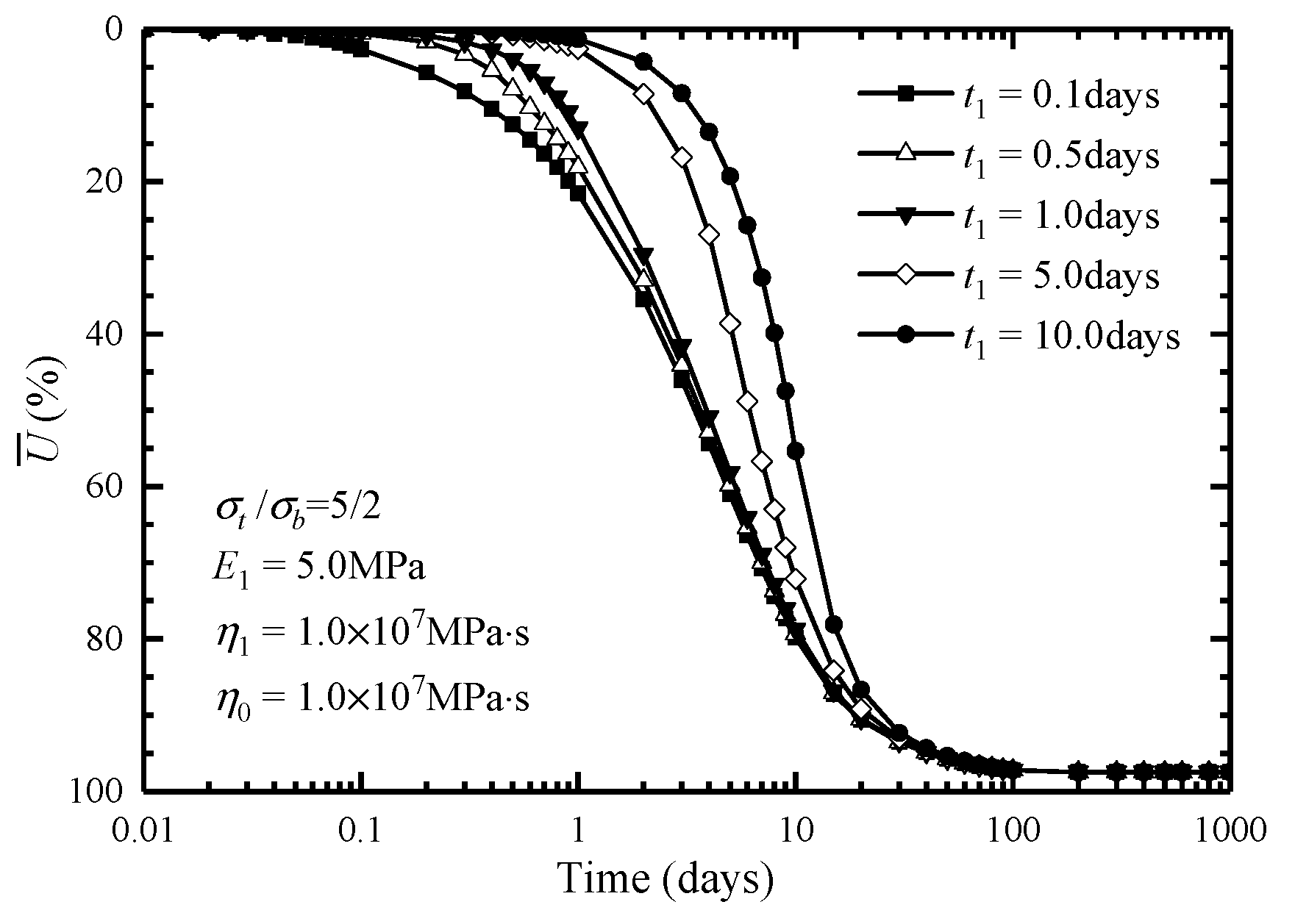
6.1. Consolidation Behavior Analysis under One-Step Loading Condition

For the solutions under the one-step loading condition, the expression of the overall average degree of consolidation $\overline{U}$ can be seen in Equations (44) and (45). In the parameter analysis, $t_1$, ${\sigma }_t/{\sigma }_b$, $E_1$, ${\eta }_1,$ and ${\eta }_0$ are selected to analyze the consolidation behavior.

Figure 5 shows the influence of loading time $t_1$ on consolidation behavior, where $t_1$ varies from 0.1 to 10 days. From Figure 5, it can be seen that the consolidation rate decreases with the increase in the loading time $t_1$ at the initial stage. When the loading time increased from 0.1 days to 10 days, the consolidation degree decreased from 80% to 55% on the 10th day. However, with the increase in time t, the overall average degree of consolidation $\overline{U}$ under different loading time $t_1$ tends to be the same.

In Figure 6, the influence of the distribution of additional stress with depth (${\sigma }_t/{\sigma }_b$) on consolidation behavior is investigated, where ${\sigma }_t/{\sigma }_b=\infty$ and ${\sigma }_t/{\sigma }_b=0$ represents that the additional stress has an inverted triangle distribution along the depth and a triangle distribution, respectively. It shows that the overall average degree of consolidation $\overline{U}$ increases with the increase in ${\sigma }_t/{\sigma }_b$ and the consolidation rate is the greatest with an inverted triangle distribution of additional stress. As ${\sigma }_t/{\sigma }_b$ increases from 0 to 2.5, the consolidation degree increases from 72% to 81% on the 10th day. The main reason for this phenomenon is that the vertical pervious boundary is located on the ground surface, so the larger the additional stress of the top surface, the faster the consolidation rate.

In Figure 7, $E_1$ varies from 0.1 to 100 MPa; thus, it shows the influence of $E_1$ (i.e., the modules of the spring in the Kelvin body) on consolidation behavior. It can be seen that the consolidation degree curves are almost identical under different $E_1$ at the initial stage of consolidation. Nevertheless, the rate of consolidation decreases and the rheological behavior becomes more and more obvious with the decrease in $E_1$ and the increase in time $t$. As $E_1$ increases from 0.1 to 100 MPa, the steady consolidation degree (i.e., maximum consolidation degree) increases from 90 to 97%.

Figure 8 shows the influence of ${\eta }_1$ (i.e., the viscosity coefficient of the dashpot in the Kelvin body) on consolidation behavior, where ${\eta }_1$ varies from $1.0\times {10}^5$ to $1.0\times {10}^9 \mathrm{M}\mathrm{P}\mathrm{a}·\mathrm{s}$. As can be seen from the figure, the consolidation curves intersect with each other. In the initial stage, the consolidation is accelerated with the increase in ${\eta }_1$; however, the consolidation rate gradually slows down in the later stage.

The influence of ${\eta }_0$ (i.e., the viscosity coefficient of the independent dashpot) on the consolidation behavior can be seen in Figure 9, where ${\eta }_0$ varies from $1.0\times {10}^5$ to $1.0\times {10}^9 \mathrm{M}\mathrm{P}\mathrm{a}·\mathrm{s}$. It can be seen that the consolidation rate increases with the decrease in ${\eta }_0$ at the initial stage, but the final overall average degree of consolidation decreases with the decrease in ${\eta }_0$. As ${\eta }_0$ increases from 1 × 10⁵ MPa·s to 1 × 10⁹ MPa·s, the consolidation degree decreases from 45% to 10% on the 1st day, while the consolidation degree increases from 78 to 100% on the 100th day.

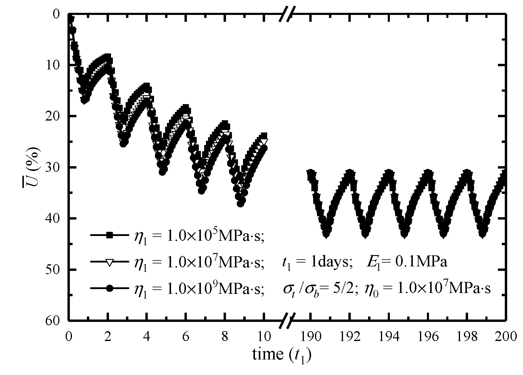
6.2. Consolidation Behavior Analysis under Cyclic Loading Condition

For the solutions under the cyclic loading condition, the expression of the overall average degree of consolidation $\overline{U}$ can be seen in Equations (62)–(65). In this chapter, the time parameters related to cyclic loads are $\alpha =0.25$ and $\beta =2.0$, and the parameters $t_1$, ${\sigma }_t/{\sigma }_b$, $E_1$, ${\eta }_1,$ and ${\eta }_0$ are also used to study consolidation behaviors.

Figure 10 shows the influence of loading time $t_1$ on consolidation behavior. It shows that the maximum degree of consolidation increases with the increase in $t_1$, while the minimum degree of consolidation decreases with the increase in $t_1$ during the cyclic loading. The consolidation degree curves tend to a steady state after a certain number of loading cycles.

In Figure 11, the influence of ${\sigma }_t/{\sigma }_b$ on the consolidation behavior is studied. It can be seen that the amount of relative variation of consolidation within each cycle becomes larger for larger ${\sigma }_t/{\sigma }_b$, and the amount of relative variation of consolidation degree within each cycle is the smallest with a triangle distribution of additional stress. With ${\sigma }_t/{\sigma }_b$ increasing from 0 to 1, the variation of the consolidation degree under cyclic loading increases from 8 to 15%.

The influence of $E_1$ on consolidation can be seen in Figure 12. From Figure 12, it can be seen that the consolidation rate is accelerated with the increase in $E_1$ at the initial stage. However, when the number of cycles increases to a certain value, the consolidation degree curves under different $E_1$ almost coincide completely.

Figure 13 shows the influence of ${\eta }_1$ on consolidation behavior. As can be seen in the figure, the effect of ${\eta }_1$ on the consolidation behavior is similar to that of $E_1$, but the effect of ${\eta }_1$ on the consolidation rate is relatively greater. The consolidation rate increases with the increase in ${\eta }_1$ at the initial stage, but the influence of ${\eta }_1$ becomes insignificant at the later stage.

The influence of ${\eta }_0$ can be seen in Figure 14. It can be seen that the consolidation rate decreases with the increase in ${\eta }_0$ at the initial stage and the amount of relative variation of the consolidation degree within each cycle is larger with smaller ${\eta }_0$ during the entire consolidation process. As ${\eta }_0$ increases from 1 × 10⁵ MPa·s to 1 × 10⁹ MPa·s, the variation of consolidation degree decreases from 55 to 13% under cyclic loading.

From these figures, it should be noted that the consolidation degree in each cycle reaches a maximum at the end of unloading and the consolidation degree is the minimum at the beginning of the loading.

7. Discussion

For the one-dimensional consolidation problem of soft soil foundation under time-dependent loading, most of the previous studies obtained numerical solutions [25,26,27,28], while the relevant analytical solutions were few and complicated [24]. In this study, a general solution for the one-dimensional consolidation of a soft soil foundation was derived. Compared with existing analytical solutions, the variable substitution method was used to obtain the governing equation, which is simple in form and easy to solve under time-dependent loading. Then, the general solution of one-dimensional consolidation was obtained by using the separation variable method. The general solution contains only one integral of the loading function, which is easy to operate in complex loading conditions. Finally, this study gave the analytical solutions of the one-dimensional consolidation of soft soil foundation under several common loading types and analyzed the consolidation behavior under one-step loading and cyclic loading. These analytical solutions provide theoretical guidance for determining construction parameters such as the loading mode, loading rate, and loading time in the preloading method for soft soil foundation treatment. This study also summarizes the change rule of consolidation degree with time under different loading parameters.

In summary, this study further expands and enriches the analytical theory of the one-dimensional consolidation of soil and provides theoretical guidance for the construction process of soft soil foundations under variable loading.

8. Conclusions

The following conclusions may be drawn from this study:

• Based on Barron’s theory of equal strain consolidation, a four-element model was used to consider the rheological characteristics of soil, and a set of analytical solutions was developed for consolidation with vertical drains under depth and time-dependent loading. The increase in additional stress is a function depending on both time and depth. It is assumed to vary linearly with depth, and several time functions are considered to represent different loading cases, which include instantaneous loading, one-step loading, multi-step loading, and cyclic loading.
• The consolidation rate is accelerated with the decrease in loading time $t_1$ and the increase in ${\sigma }_t/{\sigma }_b$ (the value of the top-to-bottom additional stress ratio). With the decrease both of the modulus of the spring in the Kelvin body and the viscosity coefficient of the independent dashpot, the rheological behavior becomes more and more obvious at the later stage of consolidation. The rate of consolidation becomes faster at an early stage but slower at a later stage, with the increase in the viscosity coefficient of the dashpot in the Kelvin body.
• For cyclic loading, the consolidation degree in each cycle reaches a maximum at the end of unloading and reaches the minimum at the beginning of the loading. When the number of cycles increases to a certain value, the variation form of consolidation degree curves will tend to be stable.

References

1. Indraratna, B. Recent advances in the application of vertical drains and vacuum preloading in soft soil stabilization. Aust. Geomech. Soc. 2010, 45, 1–43. [Google Scholar]
2. Barron, R.A. Consolidation of fine-grained soils by drain wells. Trans. ASCE 1948, 113, 718–742. [Google Scholar]
3. Hansbo, S.; Jamiolkowski, M.; Kok, L. Consolidation by vertical drains. Geotechnique 1981, 31, 45–66. [Google Scholar] [CrossRef]
4. Onoue, A. Consolidation by vertical drains taking well resistance and smear into consideration. Soils Found. 1988, 28, 165–174. [Google Scholar] [CrossRef] [PubMed] [Green Version]
5. Xie, K.H.; Zeng, G.X. Consolidation theories for drain wells under equal strain condition. Chin. J. Geotech. Eng. 1989, 11, 3–17. [Google Scholar]
6. Kianfar, K.; Indraratna, B.; Rujikiatkamjorn, C. Radial consolidation model incorporating the effects of vacuum preloading and non-Darcian flow. Géotechnique 2013, 63, 1060–1073. [Google Scholar] [CrossRef] [Green Version]
7. Deng, Y.B.; Xie, K.H.; Lu, M.M. Consolidation by vertical drains when the discharge capacity varies with depth and time. Comput. Geotech. 2013, 48, 1–8. [Google Scholar] [CrossRef]
8. Tang, X.W.; Onitsuka, K. Consolidation by vertical drains under time-dependent loading. Int. J. Numer. Anal. Methods Geomech. 2000, 24, 739–751. [Google Scholar] [CrossRef]
9. Zhu, G.F.; Yin, J.H. Consolidation analysis of soil with vertical and horizontal drainage under ramp loading considering smear effects. Geotext. Geomembr. 2004, 22, 63–74. [Google Scholar] [CrossRef]
10. Leo, C.J. Equal strain consolidation by vertical drains. ASCE J. Geotech. Geoenviron. Eng. 2004, 130, 316–327. [Google Scholar] [CrossRef] [Green Version]
11. Conte, E.; Troncone, A. Radial consolidation with vertical drains and general time-dependent loading. Can. Geotech. J. 2009, 46, 25–36. [Google Scholar] [CrossRef]
12. Lu, M.; Wang, S.; Sloan, S.W.; Indraratna, B.; Xie, K. Nonlinear radial consolidation of vertical drains under a general time-variable loading. Int. J. Numer. Anal. Methods Geomech. 2015, 39, 51–62. [Google Scholar] [CrossRef]
13. Xie, K.H.; Xie, X.Y.; Li, B.H. Analytical theory for one-dimensional consolidation of clayey soils exhibiting rheological characteristics under time-dependent loading. Int. J. Numer. Anal. Methods Geomech. 2008, 32, 1833–1855. [Google Scholar] [CrossRef]
14. Liu, J.C.; Lei, G.H.; Wang, X.D. One-dimensional consolidation of visco-elastic marine clay under depth-varying and time-dependent load. Mar. Georesour. Geotechnol. 2015, 33, 342–352. [Google Scholar] [CrossRef]
15. Wang, L.; Sun, D.A.; Li, P.C.; Xie, Y. Semi-analytical solution for one-dimensional consolidation of fractional derivative viscoelastic saturated soils. Comput. Geotech. 2017, 83, 30–39. [Google Scholar] [CrossRef]
16. Liu, X.W.; Xie, K.H.; Pan, Q.Y.; Zeng, G.X. Viscoelastic consolidation theories of soils with vertical drain well. Chin. Civil. Eng. J. 1998, 31, 10–19. [Google Scholar]
17. Wang, R.C.; Xie, K.H. Analysis on viscoelastic consolidation of soil foundations by vertical drain wells considering semi-permeable boundary. J. Yangtze River Sci. Res. Ins. 2001, 18, 33–36. [Google Scholar]
18. Huang, M.; Li, J. Consolidation of viscoelastic soil by vertical drains incorporating fractional-derivative model and time-dependent loading. Int. J. Numer. Anal. Methods Geomech. 2019, 43, 239–256. [Google Scholar] [CrossRef] [Green Version]
19. Liu, J.C.; Zhao, W.B.; Ming, J.P.; Huang, J.Q. Viscoelastic consolidation analysis of homogeneous ground with partially penetrated vertical. Chin. J. Rock. Mech. Eng. 2005, 24, 1972–1977. [Google Scholar]
20. Zhu, G.F.; Yin, J.H. Consolidation of soil under depth dependent ramp load. Can. Geotech. J. 1998, 35, 344–350. [Google Scholar] [CrossRef]
21. Lu, M.M.; Xie, K.H.; Wang, S.Y. Consolidation of vertical drain with depth-varying stress induced by multi-stage loading. Comput. Geotech. 2011, 38, 1096–1101. [Google Scholar] [CrossRef]
22. Liu, J.C.; Griffiths, D.V. A general solution for 1D consolidation induced by depth- and time-dependent changes in stress. Géotechnique 2015, 65, 66–72. [Google Scholar] [CrossRef]
23. Zhang, J.; Cen, G.; Liu, W.; Wu, H. One-dimensional consolidation of double-layered foundation with depth-dependent initial excess pore pressure and additional stress. Adv. Mater. Sci. Eng. 2015, 2015, 618717. [Google Scholar] [CrossRef] [Green Version]
24. Shan, J.; Lu, M. Analytical Solutions for Radial Consolidation of Soft Ground Improved by Composite Piles Considering Time and Depth-Dependent Well Resistance. Int. J. Geomech. 2023, 23, 04023003. [Google Scholar] [CrossRef]
25. Satwik, C.S.; Chakraborty, M. Numerical analysis of one-dimensional consolidation of soft clays subjected to cyclic loading and non-darcian flow. Comput. Geotech. 2023, 146, 104742. [Google Scholar] [CrossRef]
26. Zong, M.F.; Wu, W.B.; El Naggar, M.H.; Mei, G.X.; Zhang, Y. Analysis of One-Dimensional Consolidation for Double-Layered Soil with Non-Darcian Flow Based on Continuous Drainage Boundary. Int. J. Geomech. 2023, 23, 04022306. [Google Scholar] [CrossRef]
27. Chen, Y.; Wang, L.; Shen, S.D.; Li, T.Y.; Xu, Y.F. One-dimensional consolidation for multilayered unsaturated ground under multistage depth-dependent stress. Int. J. Numerical Anal. Methods Geomech. 2022, 46, 2849–2867. [Google Scholar] [CrossRef]
28. Cui, P.; Cao, W.; Xu, Z.; Wei, Y.; Li, H. Analysis of one-dimensional nonlinear rheological consolidation of saturated clay considering self-weight stress and swartzendruber’s flow rule. Int. J. Numerical Anal. Methods Geomech. 2022, 46, 1205–1223. [Google Scholar] [CrossRef]
29. Li, X.B.; Xie, K.H.; Chen, F.Q. One dimensional consolidation and permeability tests considering stress history and rheological characteristic of soft soils. J. Hydraul. Eng. 2013, 44, 18–25. [Google Scholar]
Figure 1. Schematic diagram for consolidation with a vertical drain.
Sustainability 15 06129 g001
Figure 2. Loading types: (a) instantaneous loading; (b) one-step loading; (c) multi-step loading; (d) cyclic loading.
Sustainability 15 06129 g002
Figure 3. Model types: (a) four-element model; (b) Merchant model; (c) Maxwell model; and (d) linear elastic model.
Sustainability 15 06129 g003
Figure 4. Model validation by consolidation test: (a) pore pressure; (b) settlement.
Sustainability 15 06129 g004aSustainability 15 06129 g004b
Figure 5. The influence of t 1 on the consolidation behavior under one-step loading.
Sustainability 15 06129 g005
Figure 6. The influence of σ t / σ b on the consolidation behavior under one-step loading.
Sustainability 15 06129 g006
Figure 7. The influence of E 1 on the consolidation behavior under one-step loading.
Sustainability 15 06129 g007
Figure 8. The influence of η 1 on the consolidation behavior under one-step loading.
Sustainability 15 06129 g008
Figure 9. The influence of η 0 on the consolidation behavior under one-step loading.
Sustainability 15 06129 g009
Figure 10. The influence of t 1 on the consolidation behavior under cyclic loading.
Sustainability 15 06129 g010
Figure 11. The influence of σ t / σ b on the consolidation behavior under cyclic loading.
Sustainability 15 06129 g011
Figure 12. The influence of E 1 on the consolidation behavior under cyclic loading.
Sustainability 15 06129 g012
Figure 13. The influence of η 1 on the consolidation behavior under cyclic loading.
Sustainability 15 06129 g013
Figure 14. The influence of η 0 on the consolidation behavior under cyclic loading.
Sustainability 15 06129 g014