Household Wealth Distribution and Its Impact in China: Evidence from the China Family Panel Studies

Abstract

As China has experienced rapid economic growth, the study of household wealth distribution has become a pressing issue. This paper uses data from the 2012–2018 China Family Panel Studies (CFPS) to examine the impact of demographic factors and urban–rural differences on household wealth distribution. The study finds that China’s household wealth Gini coefficient has increased significantly, with wealthier households accumulating wealth at a much faster rate than those at the bottom. In addition, negative wealth households, hand-to-mouth households, and indebted households have all shown an upward trend. Despite small marginal effects, demographic factors such as education, average household age, elderly numbers, and household size do not significantly affect the overall trend of the wealth distribution. Both rural and urban households at the top maintain high growth rates, but the average urban household experiences faster wealth growth than its rural counterpart. Asset allocation between rural and urban households also shows significant differences. This analysis underscores the importance of examining wealth distribution to promote equitable resource allocation and economic stability. Policymakers can use the findings of this study to reduce economic disparities and achieve the goal of common prosperity in China.

1. Introduction

After four decades of reform and opening up, China’s economy has maintained a high growth rate. As a result, people’s livelihoods have been greatly improved and poverty has been successfully reduced. At the same time, the issue of rising household wealth inequality in China has attracted increasing attention. Since the 1990s, research has been conducted on the distribution of household wealth in China. Preceding this decade, household wealth in China was largely comprised of bank deposits, and the issue of wealth inequality was relatively insignificant when compared with other countries [1,2,3]. Nevertheless, growing evidence suggests that household wealth inequality in China has reached relatively high levels and is continuing to rise. This inequality can be attributed to various factors, including geographical location, household registration, household income, family structure, and education [4,5,6]. Research on household wealth has become more abundant, especially in quantifying the inequality of household wealth distribution and studying its influencing factors [7,8,9]. However, most previous studies have mainly focused on two aspects: some have used static cross-sectional data to study static wealth distributions [1,10,11,12], while others have used comparative static data for analysis [4,13,14]. Both static and comparative static studies have certain shortcomings. Firstly, due to the differences in data collection and processing methods, it is difficult to make a direct longitudinal study under a unified framework. Secondly, due to the limitations of the short research period, it is difficult to figure out whether the influencing factors that are important in the short run still exist in the long run. Finally, it is easy to overlook the influencing factors that are important in the long run, and it is difficult to quantify the effects of these factors. Therefore, it is necessary to study the dynamics of household wealth distribution in China over a longer period using the available research data.

In recent years, both the compilation of new datasets and the application of new research methods have made significant progress, and the comparative study of wealth inequality in a global context has also made great progress. Piketty and Saez studied the long-run evolution of income and wealth inequality in Europe and the United States [15]. Alvaredo et al. conducted a systematic study of wealth distribution in major countries from 1890 to 2015 by constructing a global inequality database, which greatly facilitates the comparative study of global wealth distribution [16]. Di Matteo contributed to placing wealth inequality in a historical and comparative perspective by examining trends in wealth inequality in North Atlantic Anglosphere countries, including Canada, the United Kingdom, and the United States, from 1668 to 2013 [17].

Other scholars have focused on examining changes in the distribution of wealth in a particular country. Kuhn et al. have conducted a detailed study of wealth inequality in the United States from 1949 to 2016 by combining historical waves of the Survey of Consumer Finances (SCF) with modern SCFs that the Federal Reserve redesigned, which is important for understanding wealth inequality in the United States since World War II [18]. Other scholars, such as Keister and Moller (2000), Saez (2017), Castaneda et al. (2013), have also conducted systematic studies of the variation in household wealth and the factors affecting the distribution of wealth in the United States [19,20,21]. By combining tax and household survey data, Garbinti et al. propose a new approach to estimating wealth inequality by examining the dynamic evolution and determinants of wealth distribution in France from 1970 to 2014, and quantifying how factors such as asset price volatility, savings rates, and asset returns for different income groups affect wealth inequality, which contributes to a better understanding of the process by which inequality has significantly increased in France since the 1980s [22]. Bengtsson et al. provide empirical support for a better understanding of household wealth distribution from an economic history perspective, and the relationship among wealth inequality and industrialization and urbanization through a historical examination of wealth distribution in Sweden from 1750 to 1900 [23]. Horan et al. use wealth survey data from 1987 to 2018 to examine short- and long-term influences on household wealth in Ireland, and their study shows that wealth inequality in Ireland is mainly driven by increasing household debt and declining homeownership rates [24]. Mishra and Bhardwaj provide empirical support for understanding the relationship between changes in household characteristics and the distribution of household wealth, using the All-India Debt and Investment Survey (AIDIS) data from 1991 to 2012 [25].

Over the past three decades, many countries around the world have experienced an inevitable increase in wealth inequality, which has become far more serious than income inequality. However, because of the great differences between China and other countries in terms of national conditions, development level, etc., the diversity and complexity of Chinese households in terms of economic and social stratification are unprecedented. With the continuous reform and improvement of the market economic system, coupled with the differences in China’s economic size, population, income disparity, and regional development, it is valuable to study the wealth distribution of Chinese households and the factors that affect it systematically. The increasing availability of nationwide household survey data also facilitates the study of wealth distribution over a longer period. The focus of this paper is to conduct an exploratory study of the changing wealth distribution of Chinese residents and its determinants using data from multiple survey years.

The research innovations in this paper mainly focus on the following aspects. First, by using the CFPS data from 2012 to 2018, a more in-depth study is conducted on the distribution of household wealth in China. Second, the size and relative changes of the wealth of different types of households, such as middle-class households, households with negative wealth, “hand-to-mouth” households, and indebted households, are analyzed in detail. Third, the marginal effects of wealth inequality caused by factors such as age structure, education, elderly numbers, and household size are systematically studied by constructing a counterfactual analysis. The study of wealth inequality from a counterfactual perspective has not been covered in China, and this paper attempts to provide a useful addition to the relevant literature. Finally, a more detailed study of the size, relative change, and factors influencing the wealth of urban and rural households is conducted for urban–rural differences in China.

The article is organized as follows: Section 1 provides an introduction, Section 2 presents the data and variables, Section 3 analyzes the results of household wealth distribution, Section 4 investigates the impact of demographic factors on household wealth distribution, Section 5 explores the effect of urban–rural differences on household wealth distribution, and Section 6 concludes the study with a summary of the key findings.

2. Data and Variables

This paper uses data from the 2012–2018 China Family Panel Studies (CFPS) to examine household wealth inequality, and the impact of demographic factors and urban–rural differences on household wealth distribution. The CFPS is based on multi-level questionnaires and continuous tracking surveys of individuals and households, which breaks through the limitations of existing China survey programs that focus on a single static cross-sectional design and is innovative in the design concept, implementation, questionnaire content, and data quality [26].

The CFPS was designed and conducted by the Institute of Social Science Survey (ISSS) at Peking University, with support from the National Population Planning Commission and some Chinese universities. The CFPS questionnaire interviews were conducted using computer-assisted personal interviewing (CAPI) technology provided by the Survey Research Center (SRC) at the University of Michigan. The CFPS survey began in 2010 and is updated every two years, and the original sample currently includes 2010, 2012, 2014, 2016, and 2018. This total of five survey years of complete research data, since 2010, was the baseline survey, but there were still shortcomings in the questionnaire design, which resulted in some shortcomings in data quality, so the 2010 data were excluded. The research sample of this paper includes a total of four 2012–2018 complete survey years, and the weights of each observation year were uniformly adjusted.

The CFPS was designed to be regionally representative, so it can be considered a nationally representative sample. The initial sample size of the CFPS was 16,000 households, covering the population of 25 provinces, municipalities, and autonomous regions except Hong Kong, Macau, Taiwan, Xinjiang, Qinghai, Inner Mongolia, Ningxia, and Hainan. A total of 8000 households were obtained by oversampling from independent sub-sample frames in five provinces (“large provinces”), namely Shanghai, Liaoning, Henan, Gansu, and Guangdong, each with a sample size of 1600 households. Another 8000 households were drawn from the independent sub-sample of the other 20 provinces (“small provinces”) combined. After secondary sampling, the five “large provinces” together with the “small provinces” sample frames formed a nationally representative total sample frame.

The population characteristics in the sample data were also adjusted post hoc in a stratified manner to address the issue of inconsistency between provinces and urban–rural areas in the sample data, and to make the population characteristics in the new dataset consistent with the Chinese Statistical Yearbook. The CFPS standardized the weights for 2018 in the officially published weight data processing, and, according to its processing method, this paper adjusts the weights of previous years to maintain the same data structure of the weight data for each year. Finally, this paper constructs the new original weight data that can reflect the province, urban–rural and population factors as the basis of household wealth distribution study after the urban–rural and provincial weights and the population attribute weights are completed separately.

The CFPS provides detailed information on the assets and liabilities of households in China. Household assets are divided into several main categories: housing, cash and deposits, financial assets other than cash and deposits, productive assets, and the value of consumer durables and farmland. Financial assets other than cash and deposits can be further subdivided into several broad categories: stocks, bonds, loans, cash used in operating activities, investment in other enterprises (excluding stocks and bonds), housing provident funds, endowment insurance, and collectibles. The value of farmland is included in household wealth in this paper [9,27]. Following the calculation of the value of farmland by McKinley and Griffin (1993) [27], this paper derives the value of farmland for rural households by assuming that 25% of the total income of rural households comes from farmland, with a perpetual cash flow discount rate of 8% for farmland income. In addition, the CFPS data for each year are adjusted to the CPI for each province to be measured in 2018 prices. Household debt consists of mortgage and nonmortgage debt, which includes business loans and borrowings, debt used to purchase consumer durables, debt owed to family members for medical treatment, debt owed for other family emergencies, and student loans. Household wealth is defined as total household assets minus total household debt [4,18,20].

3. Results

3.1. Size and Composition of Household Wealth

Table 1. Changes in average household wealth in China, 2012–2018 (CNY).

	National	Urban	Rural
2012	361,257	505,968	211,713
2014	395,571	540,656	243,256
2016	518,309	689,333	297,401
2018	683,705	931,788	308,830
2012–2018 CAGR	11.2%	10.7%	6.5%

Note: Wealth is adjusted to the Consumer Price Index by province based on 2018 prices, and subsequent results are adjusted to the CPI.

shows the trend of average household wealth in China from 2012 to 2018.Although the wealth of Chinese households has maintained rapid growth, the growth rate of urban household wealth is significantly higher than that of rural households. From 2012 to 2018, the national average household wealth increased from CNY 361,000 to CNY 684,000, with an average compound annual growth rate of 11.2%, which is higher than the growth rate of China’s GDP during the same period. The wealth of China’s rural households increased from CNY 212,000 in 2012 to CNY 309,000 in 2018, with a real compound growth rate of 6.5%, while the wealth of urban households increased from CNY 506,000 in 2012 to CNY 932,000 in 2018, with an average real compound annual growth rate of 10.7%. (Based on CHIP data from the Chinese Household Income Project (CHIP), Li calculates that the per capita wealth of the national residents in 2018 is CNY 206,000 (USD 31,100), the per capita wealth of urban residents is CNY 320,000 (USD 48,300), and the per capita wealth of rural residents is 81,000 CNY (USD 12,200) [28]. This paper, measured by the average CFPS household size, corresponds to a national per capita wealth of CNY 201,000 (USD 30,300), a per capita wealth of urban residents of CNY 290,000 (USD 43,800), and a per capita wealth of rural residents of CNY 84,000 (USD 12,600) in 2018. Although the data sources are different, this paper is closer to the measurement results of Li [28].)

3.2. Gini Coefficient of Household Wealth

The wealth Gini coefficient measures wealth inequality on a scale of 0 to 1, with 0 representing perfect equality and 1 representing maximum inequality. A higher coefficient indicates greater wealth inequality.

Table 2. Change in Gini coefficient of household wealth, 2012–2018.

	2012	2014	2016	2018
National	64	70	68	73
Excluding top 1%	59	64	62	69
Excluding top 5%	53	59	56	64
Excluding top 10%	52	57	52	59
Urban	63	69	68	68
Excluding top 1%	59	65	62	64
Excluding top 5%	53	59	56	60
Excluding top 10%	49	55	50	53
Rural	58	65	62	75
Excluding top 1%	52	59	56	69
Excluding top 5%	47	55	51	65
Excluding top 10%	47	55	51	64

Note: The values in the table are the Gini coefficient in percent.

reflects the trend of the wealth Gini coefficient of Chinese households from 2012 to 2018. The first row is the wealth Gini coefficient of all households, the second row is the wealth Gini coefficient after excluding the top 1% of households, the third row is the wealth Gini coefficient of household wealth after excluding the top 5% of households, and the fourth row is the wealth Gini coefficient of household wealth after excluding the top 10% of households. The table also shows the wealth Gini coefficients of household wealth for urban and rural households separately.

Looking at the trend of the Gini coefficient of household wealth, three important conclusions can be drawn. (1) The Gini coefficient of household wealth in China showed an increasing trend from 0.64 in 2012 to 0.73 in 2018, and the Gini coefficient of wealth showed a significant increase even after excluding the top 1%, top 5%, and top 10% of households. (2) After excluding the top households, the Gini coefficient of China’s wealth showed a relatively large decrease; for example, after excluding the top 1% of households, the Gini coefficient decreased by 4% in 2018. (3) According to the urban–rural division, the Gini coefficients of household wealth within urban and rural areas still showed a tendency to increase over time. After excluding the households at the top, the Gini coefficient of wealth showed a decreasing trend. Overall, the Gini coefficient of urban households increased less, by only 5% from 2012 to 2018, while the Gini coefficient of rural households showed a more significant increase.

Table 3. Changes in wealth share and Gini coefficient of different household types, 2012–2018.

	2012		2014		2016		2018
	Share (%)	Gini Index	Share (%)	Gini Index	Share (%)	Gini Index	Share (%)	Gini Index
Housing assets	73.8	68.1	81.7	71.7	79.2	71.9	85.8	76.0
Financial assets	10.6	79.1	8.0	84.4	12.3	80.4	8.6	80.2
Other assets	21.7	76.2	17.0	87.3	17.2	74.0	13.4	74.2
Liabilities	−6.1	91.6	−6.7	91.9	−8.6	87.9	−7.8	90.1

Note: Assets in the table are positive and liabilities are negative.

shows the changes in the shares of household assets and liabilities and the Gini coefficient in percent. From 2012 to 2018, the share of housing in total household assets increased from 73.8 percent in 2012 to 85.8 percent in 2018, while the shares of financial assets and other assets decreased by 2 percent and 8.3 percent, respectively, and the share of household liabilities increased by 1.7 percent. In terms of changes in the Gini coefficients of assets and liabilities, wealth inequality has been on an upward trend. The inequality of financial assets and other assets and liabilities is also high, but the increase in the Gini coefficient is smaller than that of housing.

3.3. Share of Household Wealth

Table 4. Household wealth share trends, 2012–2018 (%).

	2012	2014	2016	2018
Bottom 50%	9.8	6.6	8.0	4.7
Bottom 25%	1.6	−0.1	0.8	−0.1
Bottom 25–50%	8.2	6.7	7.2	4.8
50–90%	39.3	38.2	37.2	38.1
50–75%	17.7	16.9	16.6	15.4
75–90%	21.6	21.3	20.6	22.7
Top 10%	50.9	55.2	54.8	57.2
Top 5%	37.4	42.1	41.5	41.6
Top 1%	16.3	20.3	19.4	17.1

shows the evolution of the share of wealth held by households at different intervals from 2012 to 2018. As can be seen, the share of wealth held by the top 10% of households increased from 50.9% to 57.2% between 2012 and 2018. On the other hand, the share of wealth held by the bottom 50% of households decreased from 9.8% to 4.7%. The share of wealth held by the bottom 25% of households fell from 1.6% to −0.1%.

The wealth share of households in the 25–50% wealth bracket declined from 8.2% to 4.8%. Households in the 50–90% bracket are the typical middle class in China, and, overall, the wealth share of middle-class households declined more slowly, from 39.3% in 2012 to 38.1% in 2018. The wealth share of households in the 50–75% bracket declined from 17.7% to 15.4%, while the wealth share of households in the 75–90% bracket increased from 21.6% in 2012 to 22.7% in 2018. Even the wealth share within the middle-class households showed a large divergence trend, with the wealth share of households in the front of the middle-class households increasing, while the share of households in the back of the middle-class households slightly decreased.

This means that the main beneficiaries of the increase in household wealth in China were the top 10% of households, while middle-class households barely maintained their wealth share, and the bottom 50% of households experienced a significant decline in their wealth share. It can be said that, from 2012 to 2018, the distribution of household wealth in China diverged: households at the top of the wealth table became richer, households in the middle of the wealth table barely maintained their wealth share, and households at the bottom of the wealth table became poorer.

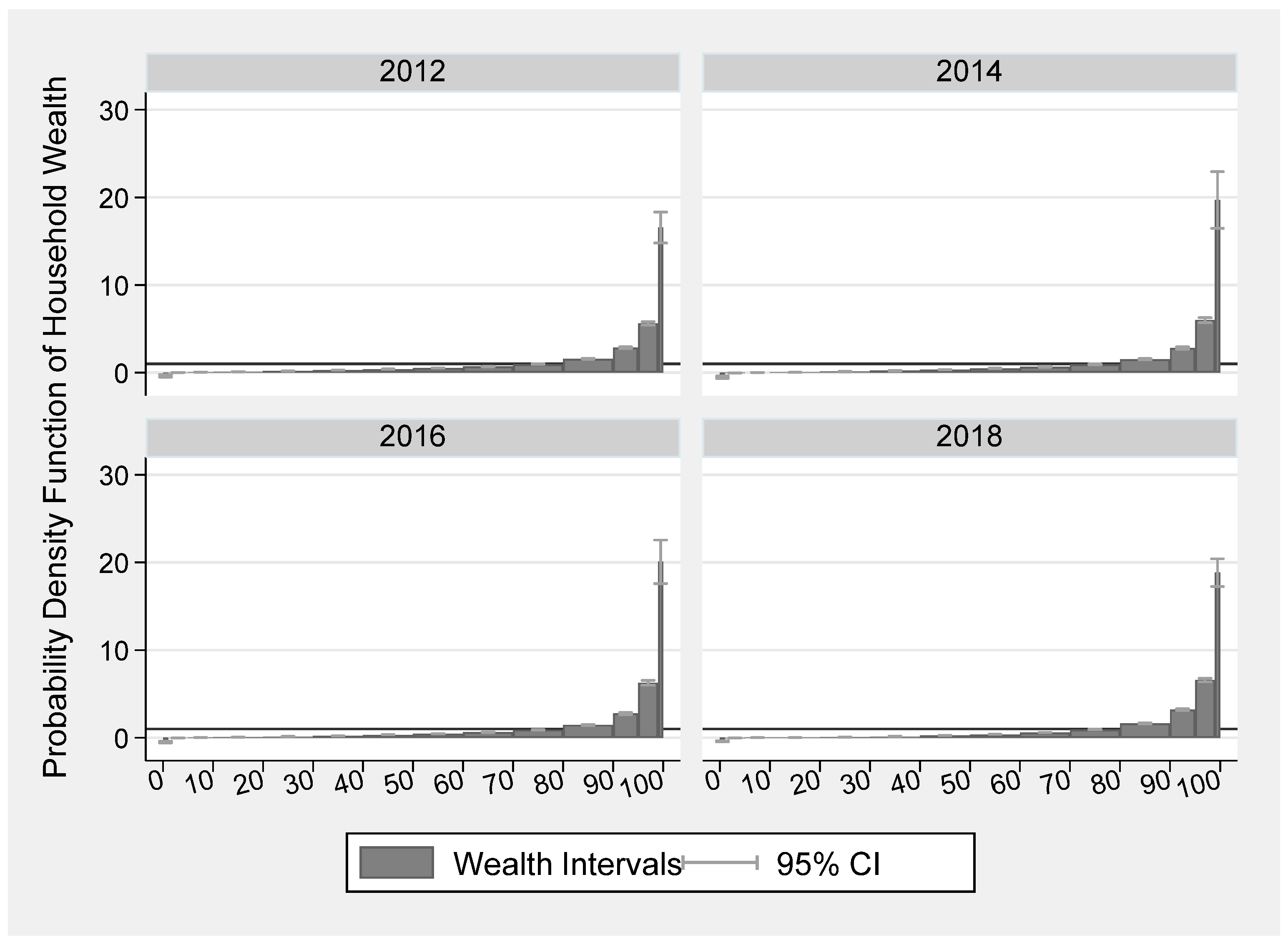
Figure 1 shows a probability density function of household wealth shares for 2012–2018, where the horizontal axis represents wealth intervals within which households fall, and household wealth is split every 10 percentage points for better representation of wealthy and poor households. The vertical axis represents the probability density of household wealth in the corresponding interval, and the width of the horizontal axis is multiplied by the height of the vertical axis to represent the share of wealth held by households in the corresponding interval.

The horizontal black line represents the absolute equality line of the household wealth distribution, above which households have more wealth relative to their share of the population, below which households have less wealth, and beyond which households have a more unequal wealth distribution. For example, in 2012, the rightmost histogram shows that the probability density coefficient for the richest 1 percent of households is 16.3, with a 95 percent confidence interval of 14.7 to 18.1, meaning that the top 1 percent of households have a wealth share of 16.3 percent and a 95 percent confidence interval of 14.7 to 18.1 percent, which is much higher than their share of the population.

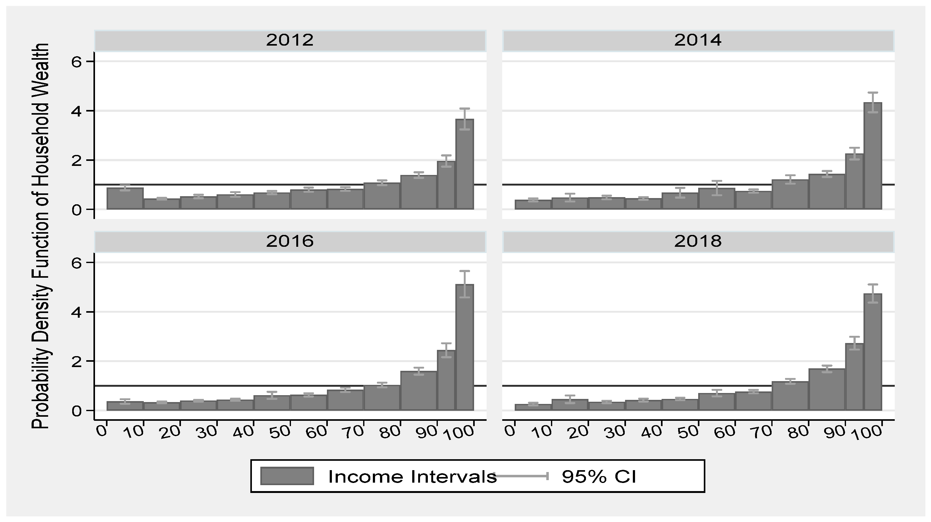
Moreover, since household wealth and income are closely related, holding asset returns and structure constant, household wealth growth equals income growth. While many studies have shown that high-income households are more likely to achieve wealth accumulation, this paper discusses the change in the share of household wealth by household income. Figure 2 is a probability density function of household wealth with the income bracket in which the household is located from 2012 to 2018. The horizontal axis is the bracket in which the household’s income is located, and income is divided into deciles from low to high, and the top 10% income range is further divided into the top 5% and 5–10% intervals.

It is also clear from the results that the right side of the probability density function is significantly higher than the left side, indicating that the share of wealth is also higher for households at the top of the income range, while it is significantly lower for households at the bottom of the income range. The paper shows that the share of wealth held by households in the top 5 percent of the income range is about 25 percent, and the results are robust at the 5 percent significance level. The share of wealth held by households in the top 10 percent of income increased from 28 percent in 2012 to 37 percent in 2018, while the share of wealth held by households in the bottom 50 percent of income decreased from 31 percent to 19 percent, confirming that household income growth and wealth accumulation are closely linked, with households at the top of the income scale accumulating wealth the fastest, and that both household income and household wealth have been clearly skewed toward the wealthy in recent years.

3.4. Top 10% Wealth Households

This section examines the size and growth rate of household wealth among the top 10 percent of households. It further subdivides the 10 percent interval into the top 5 percent and the top 1 percent, and finally identifies the household wealth of the 90th, 95th, and 99th percentiles.

The wealth of the top 10 percent of households maintained a rapid growth rate from 2012 to 2018. The left of Figure 3 shows the size of the wealth of households in each of the top 10 percent bands, measured at the 2018 price level, and shows that the average wealth of 90th percentile households was about CNY 800,000 in 2012 and grew to about CNY 1.6 million in 2018. The average wealth of 95th percentile households was about CNY 1.25 million in 2012 and grew to about CNY 3 million in 2018. The average wealth of 99th percentile households was about CNY 3.5 million in 2012 and grew to about CNY 7 million in 2018. As seen in the right of Figure 3, using 2012 wealth as a baseline, the wealth of households in each percentile grew about 2.2 times from 2012 to 2018, maintaining an average annual growth rate of about 15 percent, with 90th, 95th, and 99th percentile households growing at about the same rate.

Figure 4 plots the wealth of each of the three deciles of households in the top 10 percent against the median households. The average wealth of the 99th percentile households was about 20 times that of the 50th percentile households in 2012, increasing to 30 times in 2018; the average wealth of the 95th percentile households was about 7 times that of the 50th percentile households in 2012, increasing to 15 times in 2018; and the average wealth of the 90th percentile households was about 7 times that of the 50th percentile households in 2012, increasing to 15 times in 2018. The average wealth of 90th percentile households was about 5 times that of 50th percentile households in 2012, increasing to 7 times in 2018.

3.5. Households in the Bottom 90%

Alvaredo et al. (2017) and Saez and Zucman (2016) used tax data on wealthy households to study the wealth of the top 10 percent of households, and reached many valuable conclusions [16,29]. However, in contrast to the study of the wealth distribution of the richest group in a country, the study of the wealth distribution of the bottom 90 percent households, which constitute most of the population, must also receive sufficient attention. Indeed, the study of the wealth distribution of the bottom 90 percent of households has attracted the attention of a growing number of scholars. The study of the wealth distribution of the bottom 90 percent of households is particularly important to provide policy support for achieving the goal of common prosperity in China. Therefore, the wealth distribution of households in the bottom 90 percent of the wealth bracket are studied in more details in this section.

First, following Kuhn et al. (2020), we used three indicators to measure the change in the wealth of low-wealth households: the proportion of households with negative wealth, the proportion with wealth less than three months; income, and the proportion of indebted households [18]. The results in

Table 5. Percentage of households at the bottom of the wealth distribution, 2012–2018.

Year	Negative Assets	Wealth < 3 Months of Income	Indebted Households
2012	2.1%	7.2%	30.6%
2014	4.0%	14.6%	27.3%
2016	3.3%	6.5%	35.3%
2018	4.3%	12.8%	29.1%

show that in 2018, the share of households with negative wealth was about 4.3 percent, the share with wealth less than three months’ income was about 12.8 percent, and the share of indebted was about 29.1 percent. The share of low-wealth households has fluctuated since 2012, but, overall, it still shows a more pronounced upward trend. The ratio of household wealth-to-income of less than 0.25 (i.e., household wealth less than three months of household income) is usually considered internationally as an important cutoff, below which the ability of a household to withstand adverse exogenous shocks, such as unemployment and illness, is extremely low.

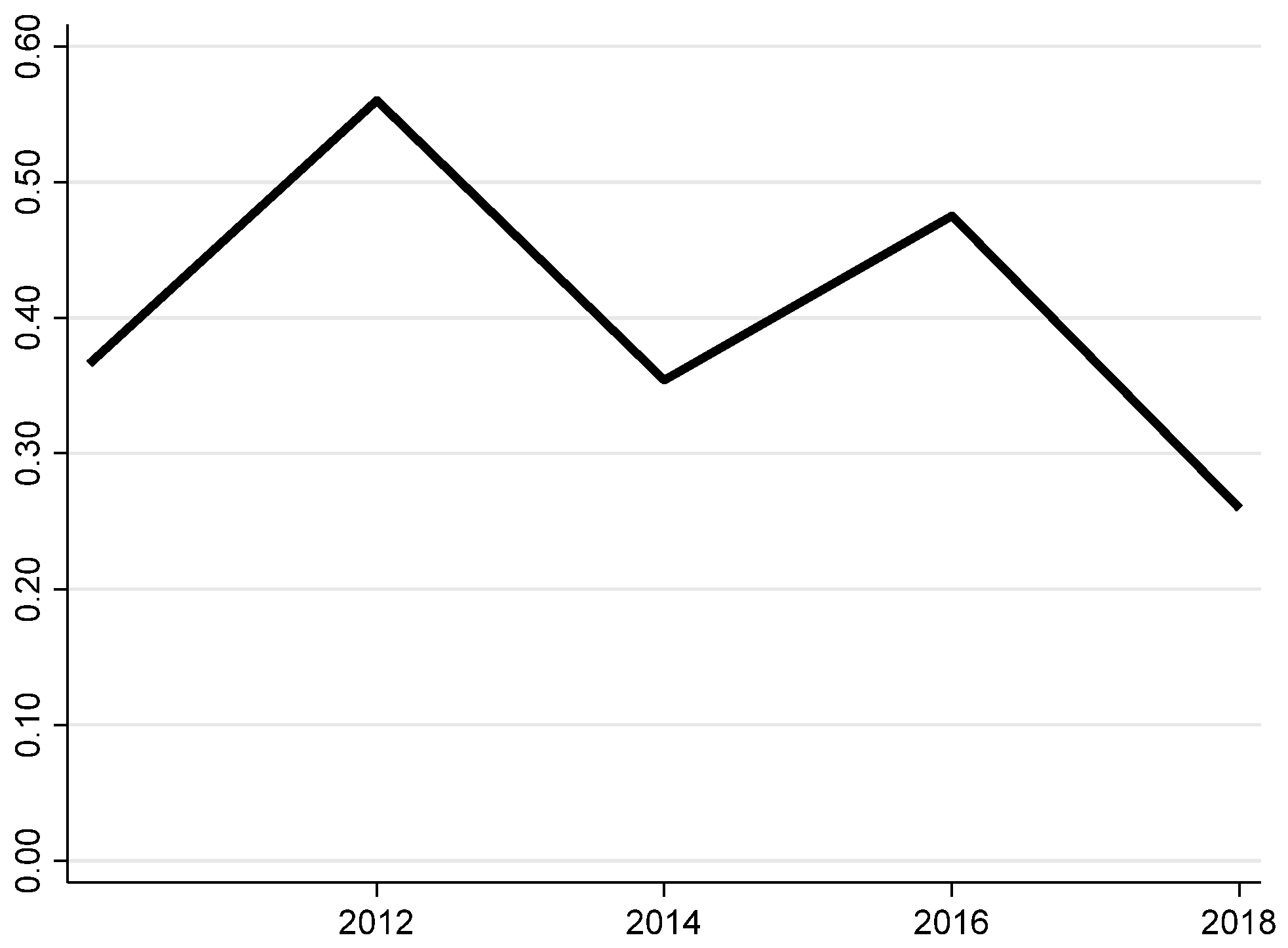
Second, housing wealth plays an important role in the overall wealth of Chinese households and is the fastest growing component of household wealth. As noted, inflation-adjusted real housing prices in China tripled between 2000 and 2020, signaling a substantial expansion of the housing market that rivals Japan’s growth during the 26-year period from 1965 to the peak of its economic bubble in 1991. This trend is significant as it suggests that China’s housing market has experienced a similar level of growth to Japan’s over the period from 1965 to the peak of its economic bubble in 1991. This phenomenon has contributed significantly to the rapid accumulation of wealth among Chinese households, particularly through homeownership and the corresponding surge in housing prices. Therefore, this paper further examined whether Chinese households with negative wealth are homeowners, and the results are shown in Figure 5. The proportion of Chinese households with negative assets that own a house from 2012 to 2018 has fluctuated, reaching the highest level in 2012; since then, the overall trend has been declining, and in 2018 it reached the lowest level, with the proportion of households being around 25 percent, about half of the proportion at the highest level in 2012. The above facts show that, under the influence of the declining proportion of homeownership among negative wealth households, the wealth growth that negative wealth households want to achieve by increasing homeownership has become increasingly difficult, and the household wealth inequality caused by housing will become increasingly serious if the housing market is not regulated effectively. In recent years, both the central and local governments in China have introduced a series of regulatory policies to curb the excessive growth of housing prices, and, fortunately, the marginal impact of real estate regulatory policies on the least affluent households is decreasing.

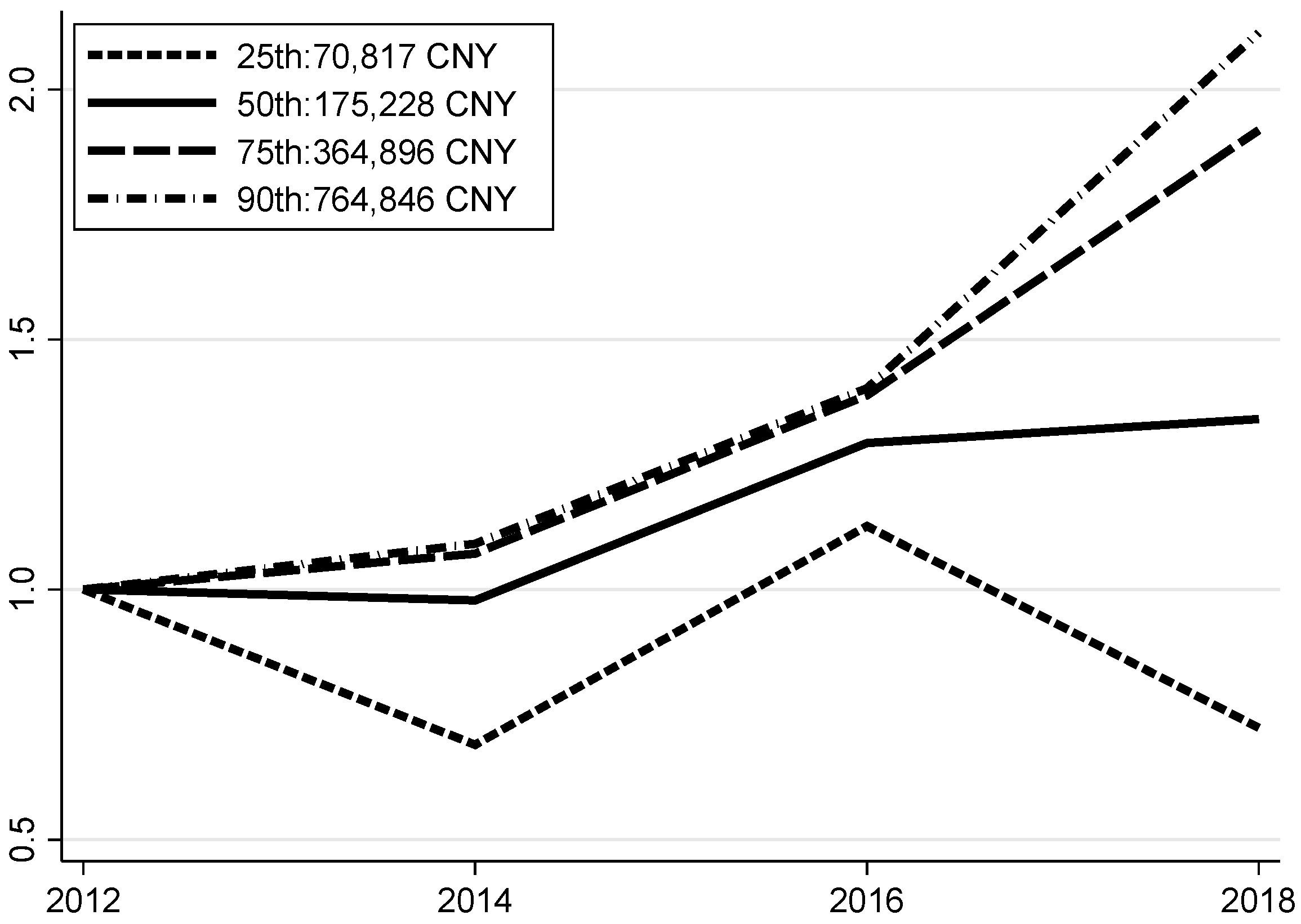
Third, Figure 6 shows the trend in household wealth for different quartiles, using 2012 as the base year, with the vertical axis showing the ratio of household wealth to the base year and showing the average household wealth for each quartile in 2012. We find that households at the top experienced faster wealth growth, with households at the 90th percentile experiencing a 110 percent increase in wealth between 2012 and 2018, compared with a nearly 80 percent increase for households at the 75th percentile and a nearly 30 percent increase for households at the 50th percentile, while household wealth at the 25th percentile remained largely unchanged. This suggests that, even excluding the top 10 percent of households, there was still a significant divergence in wealth growth across households, with households in the top quartile growing much faster than those in the bottom quartile.

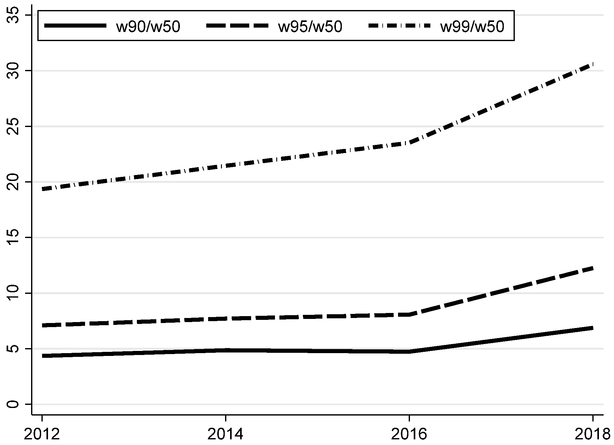
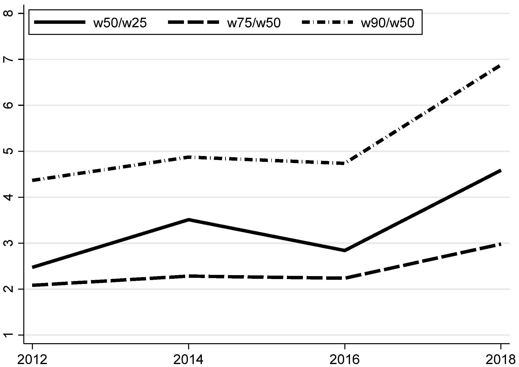
Additionally, using the relative ratio approach, the evolution of household wealth was also examined. The results in Figure 7 show that there was a large divergence in the growth rate of the bottom 90 percent household wealth from 2012 to 2018. The ratio of 90th percentile household wealth to 50th percentile household wealth increased from 4.3 to 6.8 from 2012 to 2018, the ratio of 75th percentile household wealth to 50th percentile household wealth increased from 2.1 to 3.0 from 2012 to 2018, and the ratio of 50th percentile household wealth to 25th percentile household wealth increased from 2.5 to 4.6 from 2012 to 2018. The above results reflect the remarkable fact that, in terms of wealth accumulation, the growth of the 90th percentile households was faster than the 50th percentile households, and the growth of the 50th percentile households was faster than the 25th percentile households.

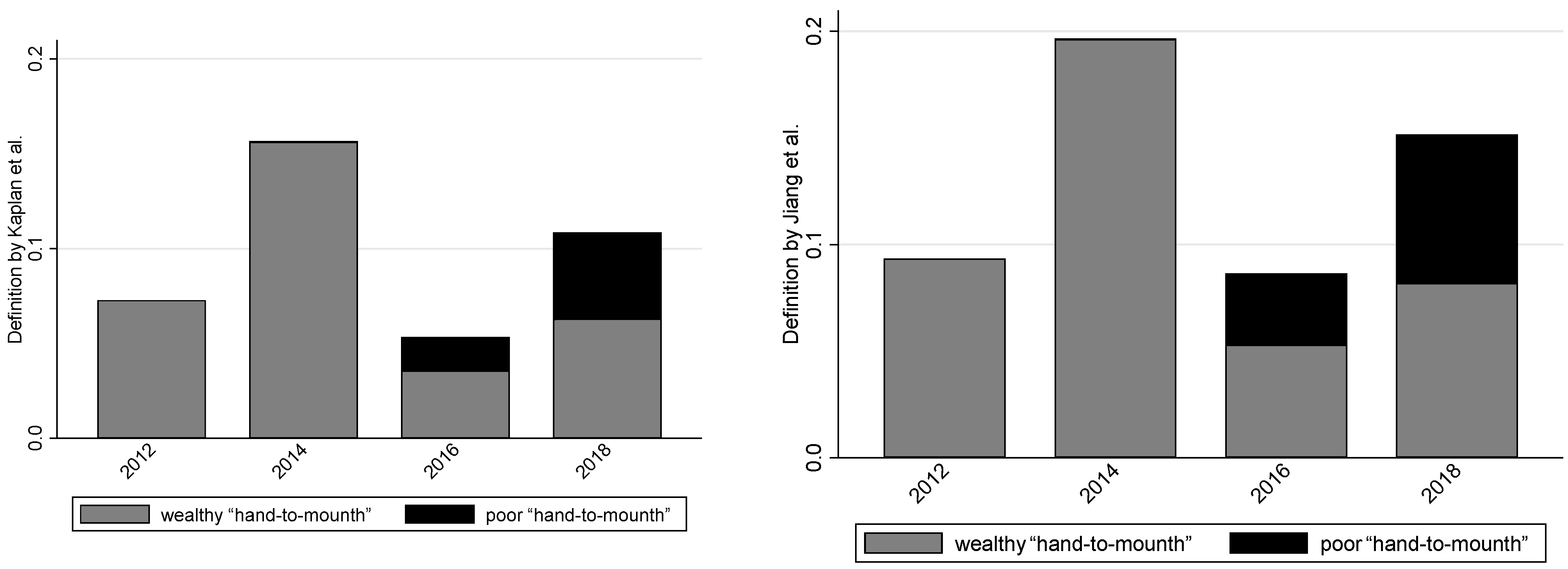
Finally, in this section, we examined household wealth by asset liquidity, as asset allocation and consumption change significantly when the composition of household wealth consists mainly of illiquid assets [30,31]. Typically, illiquid households are referred to as “hand-to-mouth” households. Following Kaplan et al. (2014), this paper defines “hand-to-mouth” households as those with positive wealth but less than a quarter of annual income [32]. We further divide “hand-to-mouth” households into wealthy “hand-to-mouth” households with positive illiquid assets and poor “hand-to-mouth” households with illiquid assets less than or equal to zero. The results in the left of Figure 8 show that hand-to-mouth households account for about 10 per cent of all households. The share of wealthy hand-to-mouth households has increased slightly in recent years, while the share of poor hand-to-mouth households has increased more significantly.

Jiang et al. (2019) argue that the internationally accepted classification method does not fit the actual situation in China [30]. This is mainly because the share of housing in the wealth of Chinese households is too high, which causes people to save more in advance to make down payments. Therefore, households whose housing wealth is positive and whose wealth is less than a quarter of their annual income should be defined as “hand-to-mouth” households. The results in the right of Figure 8 show that the share of “hand-to-mouth” households is 15 percent, and the overall trend is similar to that found in Kaplan et al. (2014) [32], but the share has increased by about 5 percentage points, mainly because the number of wealthy “hand-to-mouth” households and poor “hand-to-mouth” households has increased more significantly.

4. Changes in Demographic Factors

This section discusses the impact of changes in demographic factors (education, average household age, elderly numbers, and household size) on the distribution of household wealth. Fortin et al. discussed how to construct a counterfactual analysis to examine the process of changes in the distribution of household wealth by selecting a base year and reconstructing the coefficient weights under the assumption that demographic factors remain constant [33]. The procedure is as follows: first, select 2012 as the base year and divide the data into base year data and other year data; second, for each demographic variable, $X_d$, re-estimate its weights according to the following function.

$${\phi }_X\left(X\right)=\frac{P\left(D_Y=1|X\right)/P(D_Y=1)}{P\left(D_Y=0|X\right)/P(D_Y=0)}$$

(1)

where $D_Y$ is a dummy variable equal to 1 in the selected base year and 0 in other years. The coefficients are obtained by probit regression of $D_Y$ on all covariates $X$. Second, the coefficient ${\phi }_{X_{-d}}\left(X_{-d}\right)$ is obtained by excluding $X_d$ and then regressing it. Finally, the adjusted coefficients are obtained by the result of $\frac{{\phi }_X\left(X\right)}{{\phi }_{X_{-d}}\left(X_{-d}\right)}$. The differences between the adjusted coefficient and the coefficient without any treatment is the effect of the marginal effect of the demographic factor $X_d$.

From 2012 to 2018, China’s education, average household age, elderly numbers, and household size show the following trends. Data from the National Bureau of Statistics show that the educational level of the population increased significantly, with the population of people with a college education or higher increasing from 10.1% in 2012 to 14.5% in 2018. According to the Human Capital and Labor Economics Research Center of the Central University of Finance and Economics, the average age of the national labor force (aged 14 to 64) increased from 32.2 to 38.4 years from 1985 to 2018. The CFPS sample data also show that the average age of adults over 18 in China increased from 46.1 years in 2012 to 48.4 years in 2018.Although there are some statistical differences in caliber, they all reflect the trend that the average age of Chinese households is getting older. Data from the National Bureau of Statistics show that the trend of population aging is intensifying, with the proportion of people aged 65 and over increasing from 8.5% in 2012 to 10.9% in 2018. The average number of people per household has tended to decrease, and, according to the China Population and Employment Statistics Yearbook, the average number of people per household in China decreased from 3.16 in 2012 to 3.09 in 2018. The Gini coefficient of household wealth will inevitably be affected by the above factors.

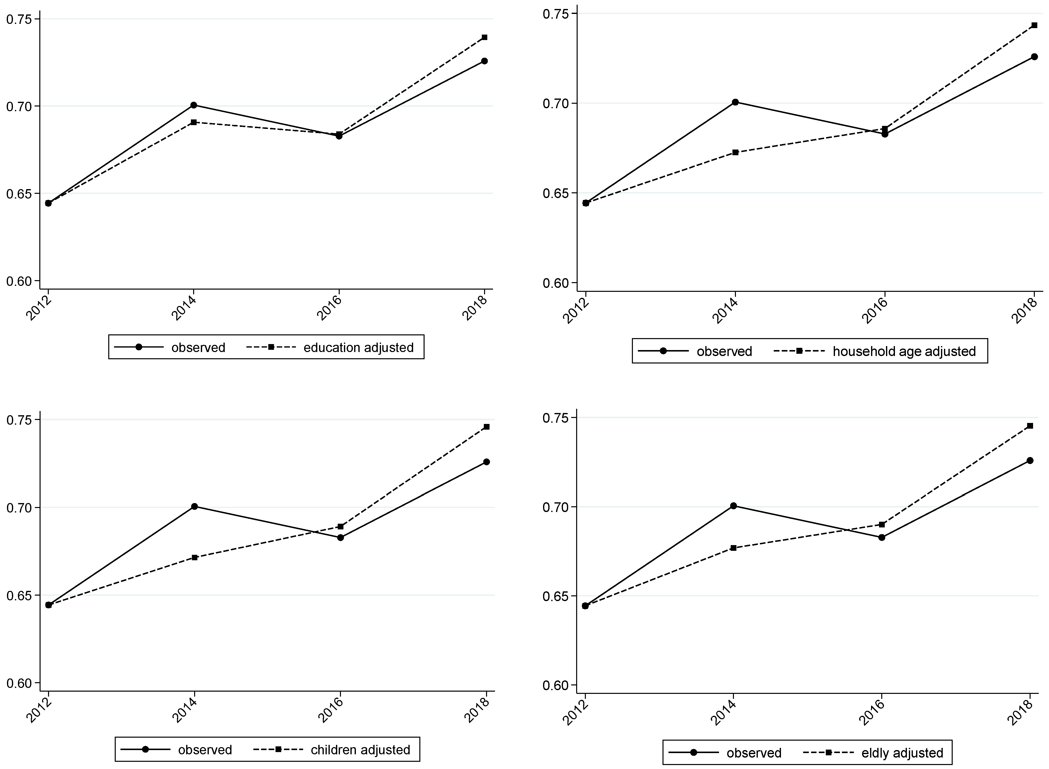
Figure 9 shows the marginal effects of education, average household age, elderly numbers, and household size on the household Gini coefficient calculated using the method of Fortin et al. [33]. The solid line shows the original wealth Gini coefficient, and the dashed line shows the wealth Gini coefficient after controlling for demographic factors. The following conclusions can be drawn from the trends. (1) The increase in education, as measured by the number of people in the household with a tertiary education or higher, has contributed to the equalization of the household wealth distribution. In 2018, the increase in education would have increased the Gini coefficient of household wealth from 0.73 to 0.74. (2) The results of the changing age structure, measured by the number of adults aged 18 and over, lead to a decrease in the Gini coefficient of household wealth by 0.03. (3) Trends in fertility, measured by the number of children in households, suggest that a decline in the number of children in households reduces the Gini of household wealth by 0.02. (4) Trends in demography, measured by the number of people over 65 in households, suggest that a decline in the number of people over 65 in households reduces the Gini of household wealth by 0.02. The counterfactual analysis of the change in the Gini coefficient associated with demographic factors suggests that the increase in education, average age of households, the decline in fertility, and the aging trend may mitigate the increase in wealth inequality, but the magnitude of the effects is quite small and insufficient to change the overall trend.

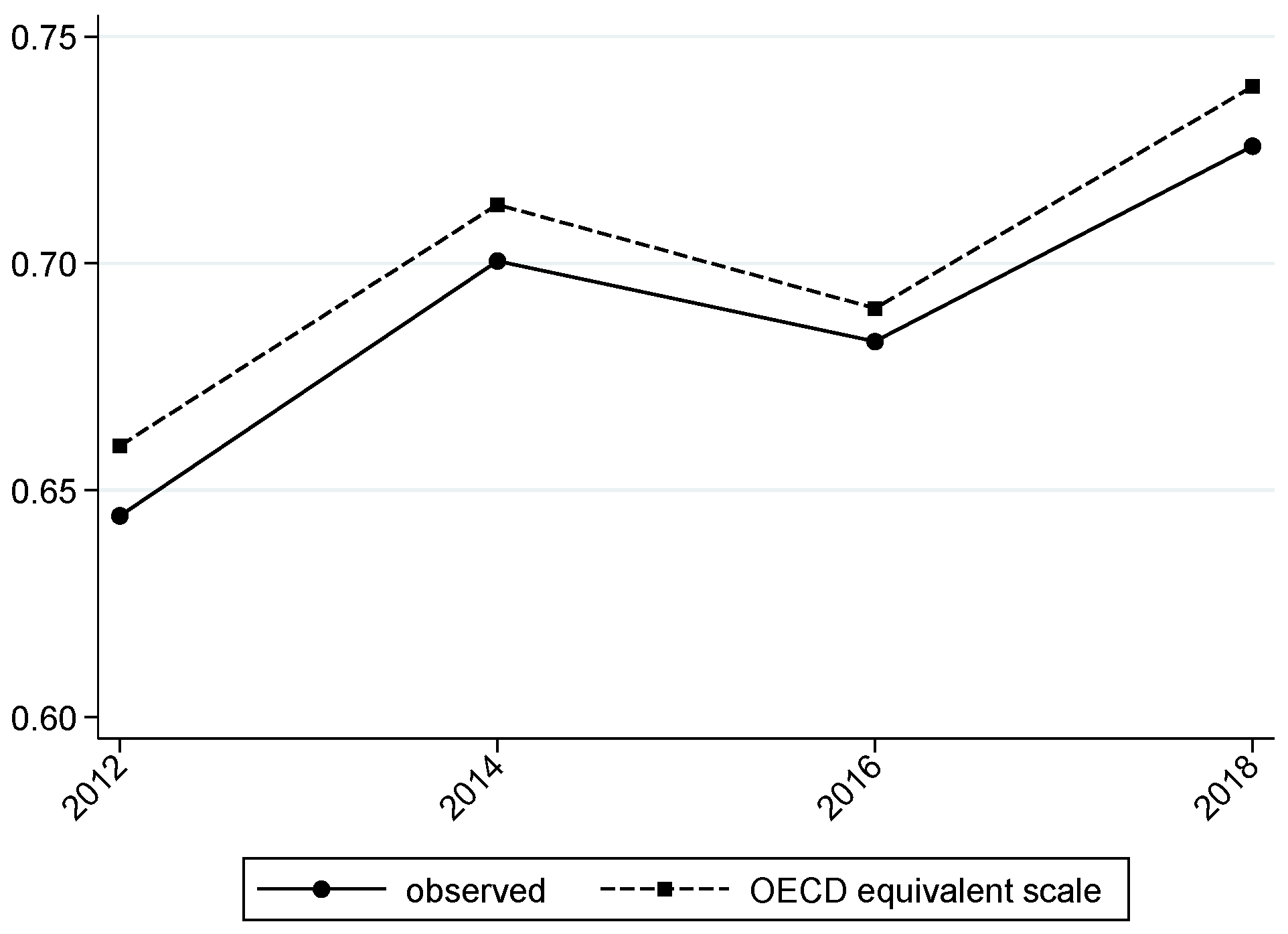
Household size has a significant impact on the calculation of the Gini coefficient of household wealth, and there are two prevailing methods of measuring household size: one is based directly on the household size counted in the observed sample, and the other is measured by calculating the equivalent population using the OECD countries, according to which the household head represents 1 equivalent person, other adults 0.7 equivalent persons and children 0.5 equivalent persons. Figure 10 shows the comparison between the Gini coefficient of household wealth per capita calculated by the equivalent person method and the wealth coefficient calculated directly. The Gini coefficient of household wealth per capita calculated using the equivalent person method is slightly higher than the Gini coefficient of household wealth per capita calculated directly, i.e., about 2 percentage points higher. However, there is no significant change in the trend between the two, with an upward trend in the Gini coefficient of household wealth from 2012 to 2018, both measured directly and using the equivalent person method.

5. Urban–Rural Differences

The urban–rural dual structure is a distinctive feature of China in economic transition, leading to large differences in household structure, consumption and saving propensities, and asset–liability structure [34,35,36,37,38]. Therefore, it is very important to study the urban–rural differences in household wealth changes in a unique country like China. Based on a comparative analysis of urban–rural wealth distribution in China, Chen argues that there is a relatively large wealth gap between urban and rural areas in China [39]. He also argues that high-wealth urban households have significantly higher risk aversion and financing ability than rural households. Similarly, Liang et al. argues that the inequality of wealth distribution among rural households has even exceeded that of urban households [14].

This section focuses on examining the changes in household wealth in China in the context of urban–rural differences. The left of Figure 11 shows the median wealth of urban and rural households from 2012 to 2018. It shows that, from 2012 to 2018, the median wealth of urban households in China was CNY 279,000, while the median wealth of rural households was CNY 123,000. The solid lines show the size of rural household wealth by year relative to the average from 2012 to 2018. The right of Figure 11 shows the change in the wealth of urban and rural households at the 90th percentile from 2012 to 2018. The average wealth of rural households at the 90th percentile was CNY 539,000, while the average wealth of urban households at the 90th percentile was CNY 1,457,000.

From the results in Figure 11, we can conclude that for households with a median income, the wealth of urban households is about 2.3 times that of rural households, and the growth rate of rural household wealth is much lower than that of urban households with a similar income. From 2012 to 2018, the wealth of rural households grew by about 50 percent, while the wealth of urban households grew by about 100 percent. The average annual compound growth rate of rural household wealth is about 5 percentage points lower than that of urban households. Since 2014, the wealth of rural households has essentially stopped growing, while the wealth of urban households has shown a sustained growth trend over the study period. For households in the top 10 percent, the average wealth of urban households is about 2.7 times that of rural households, and the wealth of households in the top 10 percent maintained a high growth rate from 2012 to 2018 for both urban and rural households, increasing by about 100 percent for both.

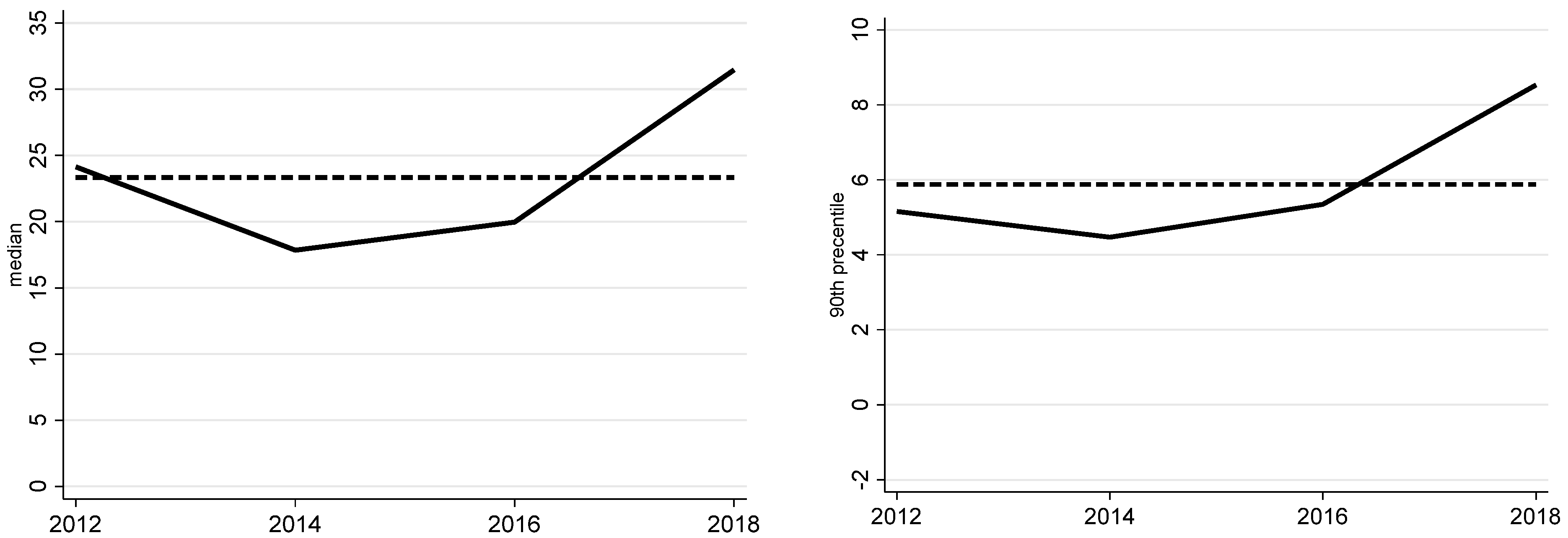
Following Kuhn et al. (2020), the relative change in the wealth of urban and rural households is measured by the rank gap, which is the percentage point difference between the rank of a given percentile in the urban and rural wealth distribution [18]. As shown in the left of Figure 12, the dashed line represents the long-term quantile trend, which is close to 25, indicating that 50th percentile urban households have the same household wealth as 75th percentile rural households. In the right of Figure 12, the dashed line is close to 6, indicating that urban households at the 90th percentile have the same household wealth as rural households at the 96th percentile.

The results also show that the solid line fluctuates around the dashed line, indicating that the urban–rural wealth gap, as measured by the ranking gap, shows a fluctuating trend from 2012 to 2018, both for the median households and the 90th percentile households. However, it is worth noting that the solid line shows an upward trend after 2014, and the ranking gap for the median household is close to 15, indicating that, for the median urban household, its wealth ranked 65th among rural households in 2014, but 80th in 2018. The ranking gap for the 90th percentile households is close to 4 percentage points, indicating that, for the 90th percentile urban household, its wealth ranked 94th among rural households in 2014, but ranked 98th among rural households in 2018. This is consistent with the findings of the distribution of household wealth under the urban–rural gap in the figure above, i.e., the wealth of urban households is growing faster than that of rural households for both the richest and the average households.

This paper is also interested in how urban–rural differences affect household wealth distribution. Therefore, it is particularly important to measure how the urban–rural gap affects wealth inequality in China. Bhattacharya and Mahalanobis pioneered the theory of decomposing income inequality by different groups [40], and Pyatt provided a solution for interpreting and disaggregating Gini coefficients [41]. According to Pyatt’s method of decomposing the Gini coefficient according to urban–rural differences, the Gini coefficient can be decomposed into three components: within-group (within urban and rural households), between-group (between urban and rural households), and overlapping term [41].

Table 6. Percentage of Gini coefficients disaggregated by urban–rural differences.

	2012	2014	2016	2018
Within	45%	47%	48%	49%
Between	38%	32%	35%	38%
Overlap	17%	21%	17%	14%

shows the percentage of each component. It shows that the results of the within-group Gini coefficient have an upward trend, increasing from 45% in 2012 to 49% in 2018. The overlap term decreases from 17% of the share in 2012 to 14% in 2018, while the contribution of between-group differences to the Gini coefficient remains unchanged. These results suggest that rising inequality within urban–rural households is the main source of the growing gap in household wealth distribution in China.

Do urban–rural differences lead to significant differences in residents’ asset choices? This question can be examined from two perspectives.

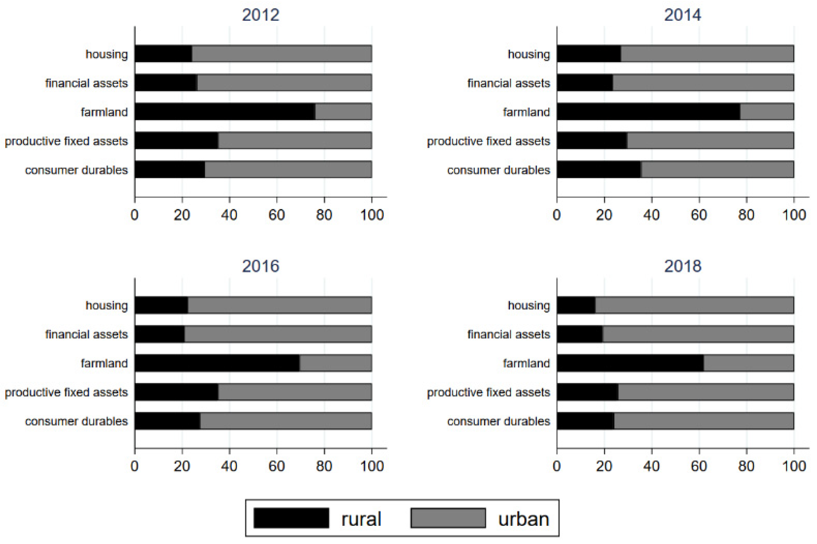
First, the share of different types of household assets in total household assets was analyzed separately for urban and rural areas, and the results are shown in Figure 13. Only the proportion of farmland assets of rural households is much higher than that of urban households; the proportion of other assets is much lower than that of urban households, and the proportion of all other types of assets except farmland tends to decline in rural households. The urban–rural differences lead to a trend of concentrating assets in urban households.

Second, using the CFPS data from 2012 to 2018, the regression analysis was conducted to determine whether the urban–rural household differences lead to systematic differences in urban–rural asset choices, and the results are shown in

Table 7. Regression analysis of urban/rural differences in asset choice.

	Housing Assets	Financial Assets	Farmland Assets	Productive Fixed Assets	Consumer Durables
logasset	7.965 ***	4.920 **	5.440 **	−7.390 ***	−5.783 ***
	(3.83)	(2.73)	(2.58)	(−9.59)	(−3.21)
logassetsq	0.123	−0.372 ***	−0.368 ***	0.328 ***	0.087
	(1.25)	(−4.19)	(−3.07)	(8.33)	(1.05)
rural	−15.560 **	−17.793 ***	54.063 ***	−3.976 *	−10.680 ***
	(−2.15)	(−3.87)	(8.88)	(−2.01)	(−2.91)
rural * logasset	0.915	1.199 ***	−3.650 ***	0.341 *	0.703 **
	(1.49)	(3.20)	(−8.29)	(2.01)	(2.55)
logfwage	−0.211	1.589 ***	−1.866 ***	−0.441 ***	0.756 ***
	(−0.47)	(7.91)	(−5.01)	(−3.90)	(3.76)
familyAge	−0.027	−0.014	−0.078	−0.012	0.150
	(−0.06)	(−0.04)	(−0.30)	(−0.17)	(1.01)
familyAgesq	0.002	0.001	−0.001	−0.000	−0.002 *
	(0.64)	(0.50)	(−0.56)	(−0.39)	(−1.77)
elderly	−3.005 ***	1.422 ***	1.655 **	0.024	−0.388
	(−3.64)	(3.25)	(2.77)	(0.12)	(−1.29)
familyEdu	0.015	−0.032	0.058	−0.010	−0.047
	(0.14)	(−0.40)	(0.64)	(−0.32)	(−1.12)
children	−0.229	−1.120 ***	0.583 ***	0.039	0.621 ***
	(−0.64)	(−6.03)	(5.12)	(0.63)	(3.97)
Time fixed effects	Yes
provinces fixed effects	Yes
N	8068	8068	8068	8068	8068
adj.R2	0.317	0.089	0.277	0.079	0.226

Notes: The explanatory variables are the share of each type of asset in the total assets of the household, expressed as a percentage, located in the first row. The explanatory variables include the logarithm of the total assets of the household (logasset) and its square (logassetsq), whether the dummy variable belongs to a rural household (rural), the interaction term of the dummy variable and the household assets (rural * logasset), the logarithm of the household wage income (logfwage), the average age of the household (familyAge) and its square (familyAgesq), the number of elderly persons over 65 in the household (elderly), and the number of children in the household (children). *, **, and *** denote coefficients that are significant at the 10%, 5%, and 1% levels, respectively, and all results control for time and province fixed effects, with t-values in parentheses after standard errors by clustering to the province level. The regression analysis methodology used in the table can also be found in the research of Boulware and Kuttner (2020) [42].

. The explanatory variables include five categories of assets, such ashousing assets, financial assets, farmland assets, productive fixed assets, and consumer durables, as a percentage of total household assets. The coefficients of the interaction term in the regression results can explain whether urban–rural differences lead to systematic differences in household asset choices. The coefficient on housing assets is insignificant, indicating that the differences between urban and rural households on housing assets is insignificant as the size of household assets increases. The coefficient on financial assets is positive and significant at the 1% level, indicating that rural households hold more financial assets, mainly cash and bank deposits, as the size of household assets increases. The coefficient of farmland assets is negative and significant at the 1% level, indicating that the share of farmland assets held by rural households decreases as the household assets increase. The coefficients of productive fixed assets and consumer durables are both positive. The former is significant at the 10% level and the latter at the 5% level, indicating that the share of both in rural households shows an increasing trend as the size of household assets increases.

As for the other control variables, the shares of financial assets and farmland assets tend to decrease and then increase, and the shares of productive fixed assets and consumer durables tend to increase and then decrease, while the share of housing assets does not change as household wealth increases. Rural households have more farmland assets than urban households, but the shares of real estate, financial assets, productive fixed assets, and consumer durables are significantly lower than those of urban households. Wages show the same trend as the shares of household financial assets and consumer durables. The number of elderly people in households shows the opposite trend to the share of housing assets and the same trend as the share of financial assets and farmland; the increase in the number of children in households shows the opposite trend to the share of financial assets, but the same trend as the share of farmland assets and consumer durables.

6. Conclusions

By combining data from the China Family Panel Studies (CFPS) from 2012 to 2018, this paper systematically examines the changes in the distribution of wealth among Chinese households and their implications. Specifically, it finds that the Gini coefficient of household wealth in China has increased significantly, the share of wealth held by households at the top has increased significantly, while the share of wealth held by households at the bottom has decreased significantly, and the majority of middle-class households have barely maintained the same share of wealth. Negative wealth, living paycheck to paycheck, and indebted families all show increasing trends. Whether measured by the growth rate of quantile wealth or the relative quantile ratio, the rate at which Chinese families accumulate wealth is accelerating toward the rich. The marginal effects of demographic factors such as education level, average household age, population aging and household size on the inequality of wealth distribution are small and do not affect the overall trend of wealth distribution. Both rural and urban households at the top continue to enjoy similar high growth rates, but average urban households are growing their wealth much faster than their rural peers, and there is a marked difference in asset allocation between urban and rural households.

Based on the above research conclusions, this paper puts forward the following policy recommendations. (1) Explore a fairer wealth tax on the super-rich whose net wealth exceeds the tax exemption thresholds. (2) Adhere to the principle that houses are for living in, not for speculation, taking effective measures to curb the rapid rise in housing prices. (3) Improve the financial market and broaden the channels of capital allocation for residents, optimize household asset portfolios, and mitigate over-dependence on housing assets. (4) Increase transfer payments to low-wealth households, enhance their education and training opportunities, and prevent the widening of wealth inequalities.

The limitations of this article lie in its use of CFPS data to examine the distribution of household wealth, which includes insufficient coverage of the super-rich, data processing using a top-coding method for assets and liabilities, and under-reporting of wealth by wealthy households for privacy reasons. Consequently, the accuracy of the conclusions is inevitably affected. Incorporating data from the Hurun Rich List to adjust the results of the CFPS, as well as integrating individual tax data into research on wealth inequality hold the potential to enhance the credibility of research findings in future studies significantly.