Rainfall Prediction Using an Ensemble Machine Learning Model Based on K-Stars

Abstract

Predicting the rainfall status of a region has a great impact on certain factors, such as arranging agricultural activities, enabling efficient water planning, and taking precautionary measures for possible disasters (flood/drought). Due to the seriousness of the subject, the timely and accurate prediction of rainfall is highly desirable and critical for environmentally sustainable development. In this study, an ensemble of K-stars (EK-stars) approach was proposed to predict the next-day rainfall status using meteorological data, such as the temperature, humidity, pressure, and sunshine, that were collected between the years 2007 and 2017 in Australia. This study also introduced the probability-based aggregating (pagging) approach when building and combining multiple classifiers for rainfall prediction. In the implementation of the EK-stars, different experimental setups were carried out, including the change of input parameter of the algorithm, the use of different methods in the pagging step, and whether the feature selection was performed or not. The EK-stars outperformed the original K-star algorithm and the recently proposed studies in terms of the classification accuracy by making predictions that were the closest to reality. This study shows that the proposed method is promising for generating accurate predictions for the sustainable development of environmental systems.

1. Introduction

Achieving sustainable economic growth is intrinsically linked to advanced climate modeling that informs policymakers about the potential risks, costs, and benefits of climate change on the economy. Predicting weather events, such as rainfall, is of great importance in this context, and it should be carefully handled. Predicting rainfall would help the planners, researchers, and technicians involved in the decision-making process of water-related issues improve sustainable management and development.

The recent study in [1] comprehensively focused on the assessment of the resilience (including the social and economic infrastructure, build environment, and institutional resilience) and livability (including the accessibility, economic vibrancy, and community well-being) of smart cities using machine learning models. For this purpose, a metric distance-based weighting approach was applied to obtain the composite scores for each aspect under the resilience and livability concepts. Then, the smart cities were sorted according to the degree of performance using fuzzy c-means clustering and six classifiers that included naïve Bayes (NB), k-nearest neighbors (KNNs), support vector machines (SVMs), classification and regression trees (CARTs), and two ensemble models, including the random forest (RF) and gradient boosting machine (GBM). The best performance in terms of the three performance measures (accuracy, Cohen’s kappa, and the average area under the precision-recall curve (AUC)) was succeeded by the ensemble GBM method. As a result of this study, the coping capacities of the cities were determined as high, medium, or low based on their clustered performance in addressing the resilience and livability paradigm. Following this concept, the aim of our study is to develop a machine learning-based strategy for rainfall prediction in the hopes that our findings will help generate a more prosperous and sustainable living environment and increase the quality of life for city residents.

Erratic rainfall can seriously threaten agriculture by undermining access to food, water, and energy. It can also trigger variable river flows and groundwater recharge, thus affecting all water sources. If a warning system informs authorities about the possibility of flooding, necessary measures can be taken in a timely manner to enhance life safety and prevent material losses in these regions. If there is a possibility of either drought or very little rainfall for a certain period, the necessary irrigation systems in these places can be established in advance so agricultural activities can operate regularly without any problems. Furthermore, water planning is another issue that needs to be addressed carefully. Properly managed and planned water storage can increase the agricultural productivity, water security, and adaptive capacity by protecting the livelihood of residents and reducing rural poverty. On the contrary, poorly planned water storage is a waste of financial resources and it could worsen the impacts of climate change. If rainfall is estimated successfully, authorities can cope with increased rainfall variability using adaptive water planning.

Rainfall prediction methods can be grouped under three categories: physical methods, statistical methods, and machine learning methods. The physical methods are conventional models that are developed using numerical weather prediction, rule-based approaches, or simulations and require a thorough description of the physical and dynamic processes of the interactions between the variables, i.e., the mathematical equations [2]. However, these models usually have a limited efficiency, computational capacity, and resolution [2]. The statistical methods aim to uncover the mathematical relationship and investigate the features of the historical time series, such as the autoregressive integrated moving average (ARIMA), the multivariate adaptive regression splines (MARS), and the Holt–Winters and hidden Markov models. However, the limitations of these conventional methods are as follows: (i) they assume that the data are stable, and therefore, the ability to capture unstable data is limited [3]; (ii) they are only suitable for linear applications and have difficulty in addressing non-linear, stochastic, and complex patterns within the data [4,5]; (iii) they require complex computing power [6]; (iv) they can be time consuming with minimal effects [6]; and (v) they are applicable to fewer parameters [4]. On the other hand, machine learning models have been used due to their ability to identify highly non-linear and irregular patterns in rainfall data [4]. The dynamic nature of the atmosphere makes machine learning methods preferable over other approaches. The superiority of machine learning models over conventional models has been proven in many studies [2,3,5]. Due to the seriousness of the issue, building a machine learning-based model is highly desirable for the sustainable development of environmental systems.

Machine learning is a branch of computer science that focuses on the use of data related to a problem domain for learning a model and finding a solution by proposing algorithms. Considering the environmental problems, its application areas cover forecasting air pollutant concentrations [7], estimating water contamination [8], forecasting greenhouse gas emissions [9], predicting soil moisture [10], modeling future changes in runoff and streamflow extremes [11], assessing the risk of resources exposed to rainfall-induced landslides [12], and many others. Rainfall prediction is one of the widely studied areas in this context. The proposed study in [13] was used to classify the rainfall status as yes or no in different zones of Ghana considering various climatic features that were collected between the years 1980 and 2019. Well-known classification algorithms, including the decision tree (DT), multilayer perceptron (MLP), KNN, RF, and extreme gradient boosting (XGBoost) were applied for this aim. The ensemble learning models were reported as the best candidates for rainfall prediction. Based on this motivation, in this study, we focus on employing an ensemble learning approach.

In this study, the aim is to predict the next-day rainfall status as “yes” or “no” considering the various meteorological attributes collected between the years 2007 and 2017 in different cities in Australia. For this purpose, the EK-stars approach, which is an ensemble of K-star classifiers, was proposed and tested using different experimental setups. The results show that our method accurately classified the rainfall data and outperformed both the original K-star classifier and the recently proposed studies.

The main contributions of this study are listed as follows:

• Rainfall prediction, which is one of the major challenges of climate modeling, was successfully handled by building a machine learning model.
• The ensembles of K-stars (EK-stars) learning approach was proposed for rainfall prediction.
• This study was original in that it proposed a probability-based aggregating (pagging) approach against bagging (bootstrap aggregating), dagging (disjoint aggregating), and boosting approaches.
• The proposed EK-stars method outperformed the standard K-star method on the same dataset.
• Compared to the state-of-the-art studies in the literature, the proposed method achieved a better classification accuracy for the rainfall prediction.

The remainder of this paper is organized as follows. In Section 2, the recent studies in rainfall prediction are briefly described. In the same section, the literature studies considering the “K-star” method are explored, along with why it was selected as the base learner of the proposed method. The methodologies and the definitions of the components of the EK-stars approach are explained in detail in Section 3. The dataset description and the statistical summary of the attributes are mentioned in Section 4. The experimental results and a general discussion are given in Section 5. The final comments and future directions are addressed in the conclusions.

2. Related Work

Using the right method for rainfall forecasting has been the primary concern of many researchers.

Table 1. Recent studies in rainfall prediction using machine learning techniques.

Ref	Year	Applied Methods	Characteristics of the Dataset	Location	The Best Result Method
[14]	2022	DT, NB, KNN, and SVM, and their combination with fuzzy logic	12 years (2005 to 2017) of weather data with 11 features (temperature, visibility, relative humidity, etc.).	Lahore, Pakistan	94% accuracy—proposed fused ML
[15]	2022	KNN, SVR, ANN, XGBoost, Stacking	Monthly rainfall series data between 1961 and 2019, large-scale climatic indices, local meteorological variables, and large-scale atmospheric variables.	Taihu Basin, China	0.532 R2—ANN (for all months)
[16]	2022	Hybrid optimized by PSO SVR, LSTM, and CNN	Precipitation time series data from 1974 to 2014 measured for 5- and 15-min time intervals.	Tehran, Iran	0.724 and 0.532 R2—LSTM for 5-min time step and 15-min time step, respectively, on the entire dataset.
[17]	2021	Neural network models based on LR, DT, RF, and statistical approach	Ten years of weather data (temperature, humidity, pressure, etc.).		84% accuracy—LR
[18]	2020	Ensemble-learning-based models, including NB, DT, SVM, RF, and ANN using average/maximum probability and majority voting as combiners	Six weather data containing temperature, relative humidity, river flow, rainfall, and water level.	Malaysia	76% precision—combination of SVM, DT, and ANN using majority voting.
[19]	2019	RF, logistic model trees (LMT), linear discriminant analysis (LDA), generalized linear model (GLM), SVM, XGBoost, GBM	Climate data for a period of 41 years on Tenerife Island considering dry or wet weather.	Tenerife, Spain	77% and 86% accuracies corresponding to training and test errors—XGBoost.

summarizes the studies [14,15,16,17,18,19] that were recently proposed on the subject of rainfall prediction by mentioning their methods, the datasets used, and the best results that were obtained. While some studies used classical machine learning methods such as the SVM [14], NB [14], and artificial neural networks (ANN) [15], some utilized deep learning methods such as convolutional neural networks (CNN) and long short-term memory (LSTM) [16]. In another study [20], the time series data (monthly rainfall data from 1951 to 2021) were handled using a hybrid deep learning technique for the monthly rainfall forecasting in China.

Rahman et al. [14] handled the rainfall prediction by using a machine learning fusion technique. The results of the machine learning models were given to another layer where fuzzy logic-based rules were applied for the final prediction. In the classification part, DT, NB, KNN, and SVM were used. The fuzzy layer contained the test data along with the output class and the predictions of the applied classifiers. The results were examined using a number of measures such as the accuracy, miss rate, specificity, sensitivity, false positive/negative value, likelihood ratio positive, and positive/negative prediction value. Their proposed fused ML algorithm managed to perform the best with a 94% accuracy in the experiments. The novelty of this study was stated as the use of machine learning fusion for real-time rainfall prediction. Adaryani et al. [16] developed deep learning-based models for short-term rainfall forecasting (5-min and 15-min forecasts). Initially, the selected models performed on the entire dataset. The LSTM achieved the best results in terms of R² as 0.724 in a 5-min time step and 0.532 in a 15-min time step and in terms of RMSE as 0.139 mm in a 5-min time step and 0.143 in a 15-min time step. The rainfall events were categorized into four classes according to their severity and duration using KNN in the event-based modeling part. This categorization step increased the accuracy of the forecasting models. In the other experiments, they also used additional predictors such as the rainfall depth differences and the rainfall depth fluctuations over shorter time stamps than the forecast lead time, which was the novel aspect of this study. These additions significantly improved the accuracies of the PSO-SVR (support vector regression optimized by particle swarm optimization) and the LSTM models. As a result of the experiments, the PSO-SVR and LSTM approaches performed better than the CNN. Balamurugan and Manojkumar [17] compared the statistical methods and machine learning models for rain prediction. It was shown that the traditional methods could not perform as well as the machine learning methods. The LR obtained a 84% overall accuracy and a 0.86 precision while the statistical approach had a 72.6% accuracy and a 0.72 precision. Aguasca-Colomo et al. [19] proposed a study to estimate the monthly rainfall as rainy or dry by considering a region with a complex orography. They used global and local meteorological parameters. Linear, non-linear, and ensemble models were selected to be used in the experiments. According to the performance metrics, the ensemble XGBoost method outperformed the other models with an 77–86% accuracy for the training/test set and a 0.34–0.54 kappa coefficient for the training/test set. They concluded that the influence of the global variables, such as the North Atlantic Oscillation index (NAO), was very low on the obtained predictive model while the local variables, such as the geopotential height (GPH), were relatively more significant than the measured variables in the meteorological stations.

Due to human nature, when it is difficult to reach a decision on a subject, the final decision is made by considering the opinions of more than one expert. In computer science, this logic is used in ensemble learning applications where, instead of sticking to the decision of a single model, a solution to that problem is offered on a common denominator by utilizing the predictive power of more than one model. In this way, the weakness of a single model for a specific problem can be supplemented by other models so that more accurate predictions can be obtained. Apart from its application in many fields, ensemble machine learning models have also been used for rainfall prediction. In the study [15], a stacking ensemble model combining different machine learning models was presented for the monthly rainfall prediction in the Taihu Basin, China using large-scale climate indices, large-scale atmospheric variables, and local meteorological variables as the predictors. The experimental studies on nine stations were conducted in five different settings, such as all the months, the annual aggregation scale, the seasonal, dry/intermediate/wet months, and the months of extreme rainfall. The R², RMSE, and MAE measures were used to evaluate the applied models, which included four base learners (KNN, XGBoost, support vector regression (SVR), and ANN) and the stacking model. According to the results, the proposed stacking model produced reasonable and satisfactory predictions in general, and in many settings, it achieved even better results than the ANN models that usually obtained good results in the literature. This study strengthened the belief that ensemble learning models can show a promising performance for rainfall forecasting. In another paper [18], ensemble learning was analyzed under three different aggregation techniques (the average probability, maximum probability, and majority voting) to predict the rainfall status. In terms of the precision, recall, and f-score metrics, different combinations of the NB, DT, SVM, ANN, and RF methods were evaluated using the voting ensemble learning strategy. The results showed that majority voting as a combiner obtained the best results among the others when the voting strategy was applied with SVM, DT, and ANN. In this direction, a learning approach based on ensemble learning is proposed in our paper using majority voting as the selected combiner.

An enhanced variation of the K-star algorithm was developed and proposed in this study for the rainfall prediction. The K-star has been applied in a wide range of areas such as agriculture [21], bioinformatics [22], surgery [23], mechanical engineering [24], civil engineering [25], and transportation [26]. The reason why the K-star algorithm was chosen as the base classifier of the proposed method is that it has achieved good results in many studies [21,22,23,24,25,26].

In one of these studies [21], plum kernel cultivars were classified by different algorithms such as a rule-based PART (partial decision tree) classifier and a tree-based LMT (logistic model trees) classifier in addition to a K-star classifier. According to the various performance metrics (accuracy, precision, f-score, Matthews correlation coefficient (MCC), etc.), the K-star acquired the highest discrimination performance metrics with significant average accuracies compared to the others. In another study [24], the classification of gear faults was analyzed by comparing three lazy learners, namely the KNN, K-star, and locally weighted learning algorithms. In terms of the classification accuracy, the optimal blending parameter was determined as 20 for the K-star classifier, which achieved the best results compared to the others. In the study [22], 58 classifiers from seven categories were tested, including Bayes, lazy, function, misc., meta, rules, and trees from the Weka package. The K-star surpassed them all for the purpose of predicting the protein thermal stability changes.

In order to identify the risky driving behaviors, the DT, RF, ANN, SVM, KNN, NB, and K-star were implemented in [26]. Only the K-star perfectly predicted all the types of driving behaviors by obtaining 100% accuracy, precision, recall, and f-score values. The prediction of the strength of the geosynthetic-reinforced subgrade soil was made using the ANN, Gaussian process regression, least median of squares regression, elastic net regularization regression, K-star, alternating model trees, M5 model trees, and random forest in [25] to construct safe and sustainable pavement structures. With even better performance than the ANN and RF, which usually achieved the best results, the K-star had a superior prediction capability compared to the others. In [23], the psychomotor laparoscopic skills of surgeons were classified using three different approaches: the radial basis function networks, K-star, and RF. According to the applied validation techniques, the K-star obtained the best mean accuracy. The comparisons with the previous methods (linear discriminant analysis, SVM, and MLP) were also analyzed considering three different tasks (the peg transfer, intracorporeal knot suture, and pattern cutting task) in terms of the accuracy, sensitivity, specificity, the area under the curve (AUC), and F1-score. The K-star outperformed all of them with the highest scores.

Apart from these studies, the K-star was applied in this paper to help solve a specific environmental problem, namely rainfall prediction. It was selected as the base learner of the proposed EK-stars method to utilize its predictive power. The key point was in selecting strong samples for the training set using a probabilistic approach in the ensemble learning phase.

3. Materials and Methods

3.1. Proposed Method

In this study, we proposed an ensemble learning approach, abbreviated as EK-stars, which combines a number of K-star classifiers for achieving a low-prediction error. It increases the selection possibility of the instances that are highly predicted by a classifier, thus both the base models and the final ensemble model converge at a strong learner. In other words, the EK-stars method increases the impact of strong training instances to prevent mislearning so that the probability of misclassification is reduced.

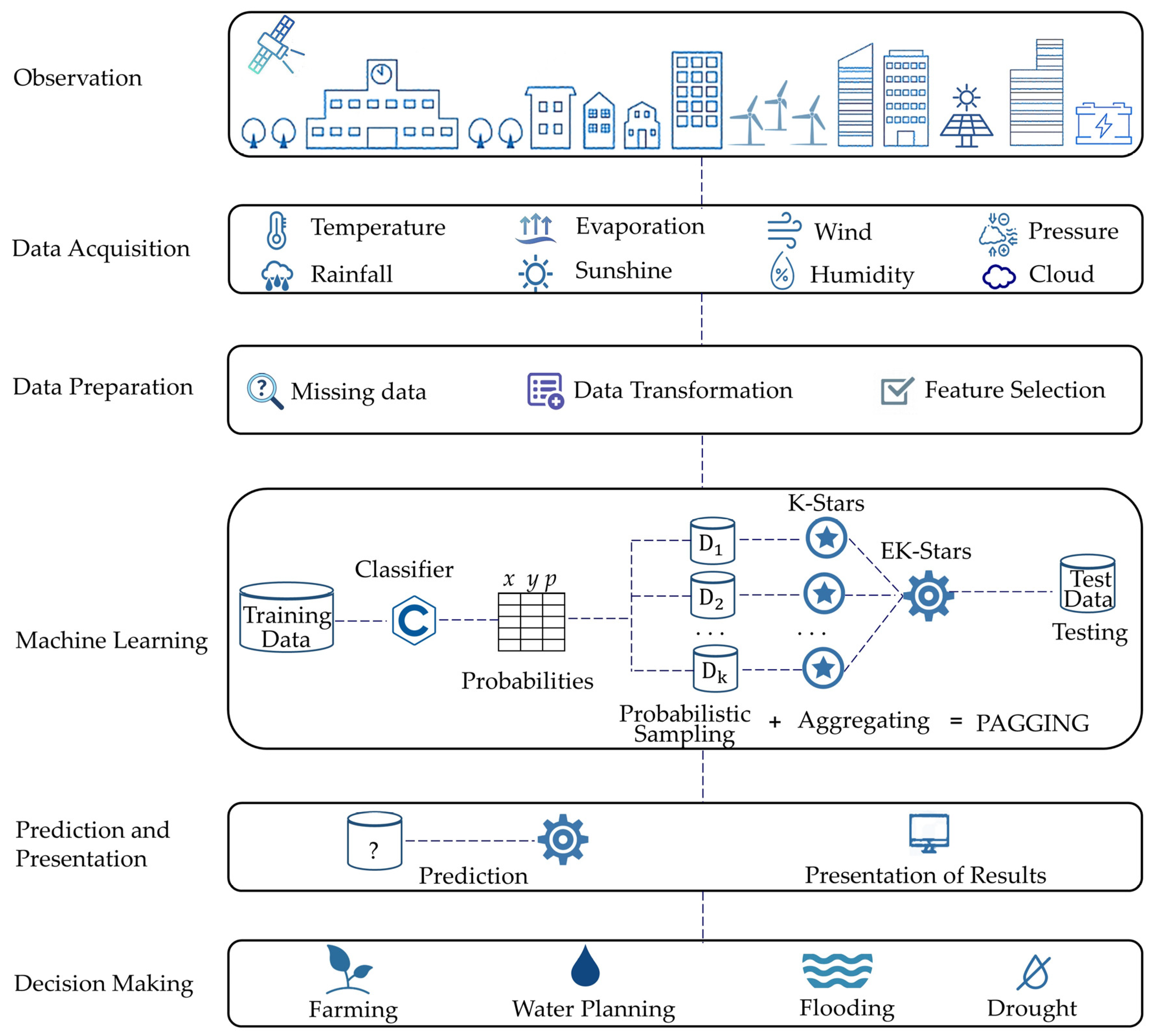
Figure 1 shows the general overview of the rainfall prediction system which uses the proposed EK-stars method. First, in the data acquisition step, the meteorological data (temperature, rainfall, evaporation, sunshine, wind, humidity, pressure, and cloud) were obtained from the observation stations, leading to the generation of big data. The collected data were stored in a cloud environment to be accessed wherever and whenever required. In the next step, the data were passed through a data preparation stage which included the missing data elimination, data transformation, and feature selection. Then, data were prepared for the implementation of the EK-stars method. In the training phase, the EK-stars method built a classifier based on the training set and then computed the classification probability for each instance by using the classifier. The classification probability is the probability of an instance being assigned to a category. After that, the method randomly selected a subset of instances using a probability-based strategy. The method increased the likelihood of the observations that were highly predicted by a classifier by a factor that depended on the classification probability. It should be noted here that the randomness in the probabilistic sampling ensured that each model in the ensemble would be trained on different instance subsets to promote diversity. Multiple training sets were generated from the original data. After that, a K-star model was built on each probabilistic sample. In the testing stage, another set of data was utilized to assess the accuracy of the developed ensemble model. In the prediction phase, an output for previously given unseen data was produced using majority voting on the decisions of the individual K-star models in the ensemble, which were built on the training sets generated using probabilistic sampling. After that, the predicted result was ready to be presented as an assistant to the decision-maker in a way that the prediction could be utilized for many different purposes, including water planning, flood prevention, and farm improvement.

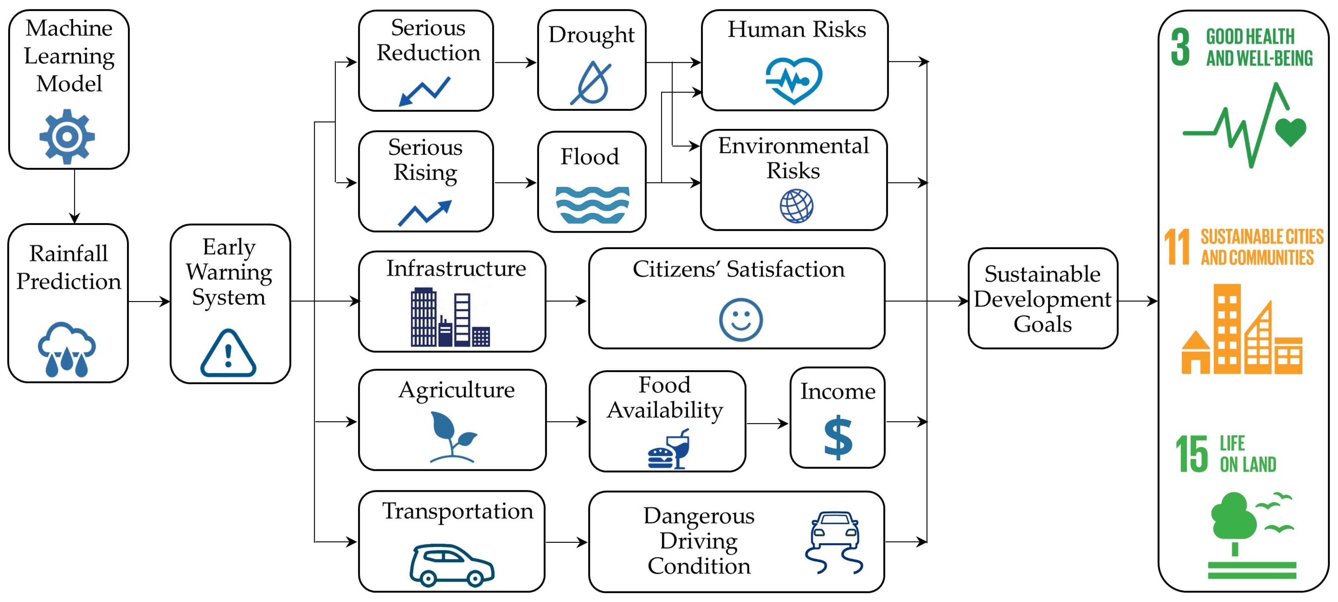
Our study meets the Sustainable Development Goals (SDG) adopted by the United Nations in 2015 in three aspects, namely for “Good Health and Well-Being”, “Sustainable Cities and Communities”, and “Life on Land”, as shown in Figure 2. In case of low rainfall, water resources are likely to decrease over time. Inaccessibility to water in this case may trigger the risk of epidemic diseases. In addition, in regions where there is very low precipitation and high temperatures, drought and wind erosion could occur. On the other hand, when a dramatic increase is observed through early warning systems, flood control could be managed in advance to possibly prevent loss of both life and property. Since the system powered by the proposed machine learning model could detect the rainfall status in advance, human risks and environmental risks could be prevented without serious consequences by serving the “Good Health and Well-Being” and “Life on Land” purposes.

In times of heavy rainfall, urban infrastructure can be seriously affected to an extent that drainage systems become overwhelmed and structural damage to the buildings becomes highly probable, resulting in an increased disruption. In terms of urban transportation, there is a possibility of dangerous driving conditions, as unexpected precipitation can cause vehicles to slip on the highway. Our predictions can act in these scenarios as a decision support system (DSS) that helps to determine the urban areas where stronger infrastructure resources should be spent, improve protective measures for preventing accidents caused by heavy rainfall on highways by meeting the “Sustainable Cities and Communities” goal, and provide citizens’ satisfaction and prosperity.

Another consideration could be observed in agricultural activities. Plants, agricultural products, and crops need different amounts of water to produce an efficient yield. Rainfall is the most important water resource used in agriculture and its accurate prediction is significant. At this point, an early warning system, supported by our machine learning model, can help the commissioned agricultural authorities take the necessary precautions for low/high precipitation situations. For example, if a dry period is expected, the necessary irrigation systems could be activated on time for the products that need more water, or on the contrary, when high precipitation is expected authorities could use the systems that will reduce the humidity for the products that require less moisture. On this occasion, the food availability for citizens could increase in direct proportion to the increase in the agricultural yield. Furthermore, economic development could be achieved with an increase in the income generated from agriculture. Therefore, both the “Life on Land” and “Sustainable Cities and Communities” aspects could be met as a consequence by our study.

3.2. Formal Definitions

Suppose there is a dataset $D$ with $n$ data instances such that $D={\left\{d_i\right\}}_{i=1}^n=\left\{d_1,d_2,\dots ,d_n\right\}$. A data instance $d_i$ consists of an input vector $x_i$ and its corresponding output $y_i$ such that $d_i=\left(x_i,y_i\right)$. The input $x_i$ is an $m$-dimensional vector with the feature values $F=(F_1,F_2,\dots ,F_m)$ Therefore, $x_i$ can be denoted as $x_i=\left(x_i^1,x_i^2,\dots ,x_i^m\right)$, where $x_i^j$ is the value of the $j$-th attribute of the $i$-th data sample. The output $y_i$ is one of the $L$ distinct class labels such as $y_iϵY=\left\{c_1,c_2, \dots ,c_L\right\}$. Here, $y_i=c_j$ means that the data instance $d_i$ belongs to the $j$-th class in the pre-defined label set. The aim of the EK-stars method is to learn a mapping function $f:X\to Y$ between the input space $x_i ϵ X$ and output space $y_i ϵ Y$ to minimize the prediction error.

The primary aim of the EK-stars method is to improve the accuracy by taking advantage of the strengths of ensemble learning in handling a classification problem. To create an ensemble $E$, the algorithm generates several new training sets $\left\{D_1,D_2,\dots ,D_k\right\}$ from the original dataset $D$ based on a systematic sampling approach, called probabilistic sampling.

Definition 1. (Probabilistic Sampling)

Probabilistic sampling refers to selecting a sample from a collection of observations based on the principle of giving a higher chance of being selected to the instances with a high probability.

The algorithm builds an initial classifier, and then calculates the probability distribution over all the classes for a given query instance $x_i$ using this classifier, and finally finds the highest probability as given in Equation (1).

$$p\left(x_i\right)=\mathit{arg}\underset{jϵ\left\{1,\dots ,L\right\}}{\mathit{max}}p(x_i|c_j)$$

(1)

where $p\left(x_i\right)$ is the maximum probability that a given data instance ($x_i$) can assign to a class, and $p(x_i|c_j)$ is the probability that instance $x_i$ belongs to the class $c_j$. The maximum probability values for all the data instances $P=\left\{p_1,p_2,\dots ,p_n\right\}$ are computed to be used in the selection of the samples which will be utilized to construct the models in the ensemble. All the data instances have a different likelihood of being selected as the sample and a conclusion can be drawn from the sample set involving the strong instances.

Definition 2. (Strong Instance)

A strong instance is an observation that can be classified by a model with a high probability.

Definition 3. (Probabilistic Sample)

A probabilistic sample $D_i$ is a collection of $n$ instances, where each element is randomly selected from the original dataset $D$ using replacement by considering their classification probabilities $P$.

It is expected that a probabilistic sample will mostly consist of the strong instances. In other words, the instances with a higher probability possess a higher chance of selection. In contrast, weak instances have the lowest probability values, and the algorithm aims to select these observations as minimally as possible. If a data instance has a low probability of being classified as a label, this means that it is an uncertain observation, so, it may cause the model to learn incorrectly during the training phase.

The proposed EK-stars method constructed a collection of K-star classifiers such that each one is built on a different probabilistic sample $D_i$. In this article, we proposed a new type of ensemble learning approach, called pagging, to encourage the method to give more credit to the stronger samples as defined in Definition (4).

Definition 4. (Probability-based Aggregating—Pagging)

Probability-based aggregating (pagging) is an ensemble learning approach that generates multiple prediction models, denoted by $E=\left\{M_1,M_2, \dots ,M_k\right\}$, on the probabilistic samples (randomly selected—probably strong—instances by considering their classification probabilities). Each model $M_i$ produces an output for a given input $x$, and the majority result or average result is taken to make the final decision.

Pagging utilizes the strong instances with high classification probabilities. This means that the instances with a high classification probability have a more significant impact on the construction of the predictive model compared to the instances with a low classification probability. The classification probability is the probability that an instance will be classified into a class.

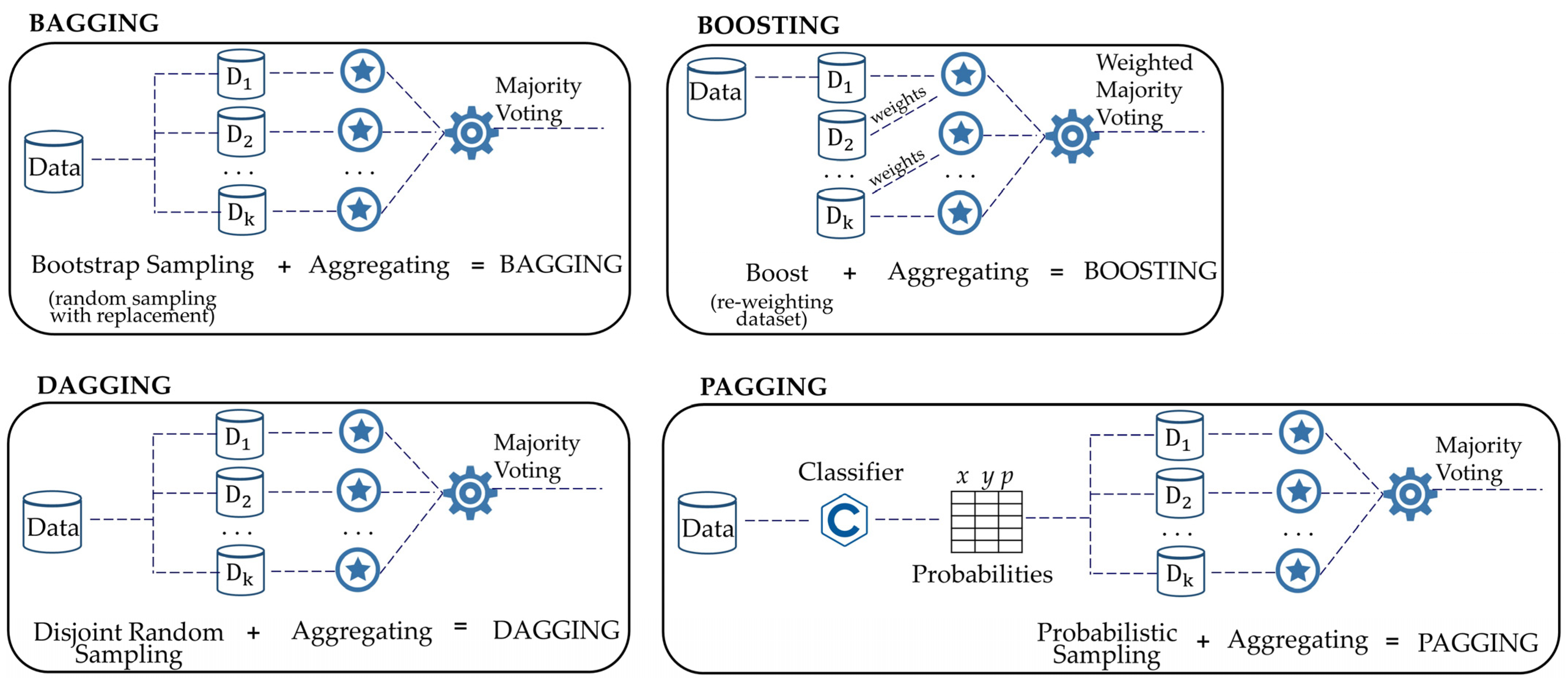
Figure 3 illustrates the differences between the bagging, boosting, dagging, and pagging techniques. Bagging (bootstrap aggregating) creates multiple training sets by taking random samples using replacements (bootstrap sampling) from the original dataset and building one classifier on each bootstrap sample. On the other hand, dagging (disjoint aggregating) generates a number of disjoint and stratified folds from the data and uses the base learning algorithm for each part of the data such that each dataset has samples that differ from the others. Boosting sequentially adds ensemble members by identifying the errors for the weighting and gives priority to the classifiers for the weighted voting. There are two major differences between pagging and the others. Firstly, pagging builds an initial classifier to determine the classification probabilities for each instance. Secondly, it uses a function that increases the chance for the instances to be selected as a training sample during the sampling process, which are predicted by the initial classifier with a high probability. Majority voting is the common step for pagging, bagging, dagging, and boosting and corresponds to the “aggregating” phase.

In ensemble $E$, the $i$-th model ($M_i$) is trained on the $i$-th dataset ($D_i$). In the classification step, a sequence of the classification models $\left\{M_1,M_2, \dots ,M_k\right\}$ is considered to make a prediction using a voting mechanism. The equation for the majority voting is as follows.

$$\hat{\mathrm{E}}\left(x\right)={\mathit{arg} \mathit{max}}_{\mathrm{c}}{\displaystyle \sum }_{i :c=M_i \left(x\right)}^{k}1$$

(2)

where $M_i\left(x\right)$ is the output predicted by the $i$-th model, $k$ is the ensemble size, $c$ is a class label, and $\hat{\mathrm{E}}\left(x\right)$ is the final predicted class that maximizes the equation for a given input $x$.

Definition 5. (EK-stars)

The EK-stars is a pagging approach that combines a number of K-star classifiers to achieve a low-prediction error.

One of the advantages of the EK-stars method is that it builds K-star classifiers on strong samples as an alternative to bootstrap samples. Due to the application of probabilistic sampling, we expect that the K-star models will be built on strong samples; thus, a prediction performance improvement could be achieved through the ensemble of all the classifiers.

Algorithm 1 presents the pseudo-code of the proposed EK-stars method. In the first step, a classifier ($H$) is built on the original training set $D$. After that, the maximum classification probability ($P_i$) is found separately for each instance. At the same time, the cumulative total is assigned to each instance. In this way, the EK-stars method decreases the likelihood of low-classified instances and increases the chance of the instances that are predicted with a high probability, which increases the focus on the strong instances. As a result, the first loop produces a cumulative probability list ($C$). In the next main loop, a new training dataset $D_i$ is created using probabilistic sampling at each $i$-th iteration. Here, a random number is generated $n$ times to choose the instances for the generation of a new training dataset for each ensemble iteration. The algorithm gives more selection chances to the instances that are classified with a high probability in order to overcome the class noise problem. Class noise can not only affect the complexity of the learned models but also the learning performance. The EK-stars method increases the selection likelihoods of the certain learning samples and decreases the selection of the uncertain learning samples. The algorithm builds $k$ models $\left\{M_1,M_2, \dots ,M_k\right\}$ on the probabilistic samples $\left\{D_1,D_2,\dots ,D_k\right\}$, which are added to the ensemble $E$. Finally, to classify an input sample $x$, the models under $E$ are utilized and each predicts an output for that sample. The final output is then determined using a voting mechanism, i.e., majority voting.

Algorithm 1. Ensemble of K-stars (EK-stars)

Inputs:        D: the dataset D = {(x1, y1), (x2, y2), …., (xn, yn)}        k: ensemble size        x: a given input to be classified Outputs:        E: ensemble model        Ê(x): the predicted class label for an input sample x

Begin:        H = Train(D)        cumulative = 0        for i = 1 to n do              pi = ClassificationProbability(H, xi)              cumulative = cumulative + pi              C.Add (cumulative)        end for        E = Ø        for i = 1 to k do              for j = 1 to n do                      rnd = Random(0, C(n))                      for q = 1 to n do                              if rnd <= C(q)                                     Di.Add(xq, yq)                                 break                         end if                      end for              end for              Mi = KStar(Di)               E = E ∪ Mi        end for        $\hat{\mathrm{E}}$$(x) = {\mathit{arg} \mathit{max}}_{\mathrm{c}}{\displaystyle \sum }_{i :y= M_i \left(x\right)}^{k}1$  End Algorithm

The time complexity of the EK-stars algorithm is O(k. L(n) + T), where k is the ensemble size, L(n) is the time needed for the execution of a classification algorithm on n instances, and T represents the time required for the probabilistic sampling process.

4. Dataset Description

The experiments were carried out on the rainfall data obtained from the kaggle.com web page [27]. The dataset includes the observations related to the meteorological variables between the years 2007 and 2017. The data from 26 regions of Australia were considered in the experiments, and their locations are shown on the map in Figure 4.

The statistical summary of the features is given separately in

Table 2. Continuous features.

Feature	Description	Unit	# of Missing Data	Min	1st Qrt.	Mean	3rd Qrt.	Std. Dev.	Max
MinTemp	The lowest temperature in degrees	°C	637	−8.5	7.6	12.1864	16.8	6.40328	33.9
MaxTemp	The highest temperature in degrees	°C	322	−4.8	17.9	23.2268	28.2	7.11762	48.1
Rainfall	The amount of rain recorded during the day	mm	1406	0	0	2.34997	0.8	8.46517	371
Evaporation	Class A pan evaporation in 24 h until 9 a.m.	mm	60,843	0	2.6	5.46982	7.4	4.18854	145
Sunshine	The number of hours of radiant sunshine in the day	hours	67,816	0	4.9	7.62485	10.6	3.78152	14.5
WindGustSpeed	The speed of the strongest wind gust in the 24 h to midnight	km/h	9270	6	31	39.9843	48	13.5888	135
WindSpeed3pm	Wind speed averaged over 10 min before 3 p.m.	km/h	2630	0	13	18.6376	24	8.80335	87
WindSpeed9am	Wind speed averaged over 10 min before 9 a.m.	km/h	1348	0	7	14.0020	19	8.89334	130
Humidity3pm	Humidity at 3 p.m.	%	3610	0	37	51.4826	66	20.7978	100
Humidity9am	Humidity at 9 a.m.	%	1774	0	57	68.8438	83	19.0513	100
Pressure3pm	Atmospheric pressure reduced to mean sea level at 3 p.m.	hpa	13,981	977.1	1010.4	1015.26	1020	7.03668	1039.6
Pressure9am	Atmospheric pressure reduced to mean sea level at 9 a.m.	hpa	14,014	980.5	1012.9	1017.65	1022.4	7.10548	1041
Cloud3pm	Fraction of sky obscured by cloud at 3 p.m.	oktas	57,094	0	2	4.50317	7	2.72063	9
Cloud9am	Fraction of sky obscured by cloud at 9 a.m.	oktas	53,657	0	1	4.43719	7	2.88702	9
Temp3pm	Observed temperature at 3 p.m.	°C	2726	−5.4	16.6	21.6872	26.4	6.93759	46.7
Temp9am	Observed temperature at 9 a.m.	°C	904	−7.2	12.3	16.9875	21.6	6.49284	40.2

and

Table 3. Categorical features.

Feature	Description	% of Missing Data	Cardinality	Mode	Mode Freq.
Date	Date on which the measurement was done	0	3456	2013-12-12	49
Location	Location name of the weather station	0	49	Canberra	3418
WindGustDir	Direction of the strongest wind gust in the 24 h to midnight	0.065114	17	W	9780
WindDir9am	The direction of the wind at 9 a.m.	0.070134	17	N	11,393
WindDir3pm	The direction of the wind at 3 p.m.	0.026443	17	SE	10,663
RainToday	“Yes” if precipitation exceeded 1 mm, otherwise “No”	0.010013	3	No	109,332

for the numerical and categorical attributes, respectively. In the training dataset, the “RainTomorrow” values were assigned as yes if the amount of the next-day precipitation was above 1 mm, otherwise they were attributed as no. The aim was to correctly predict the target attribute “RainTomorrow” for a given day by considering the input variables. In other words, for the given input variables regarding a day, a forecast for whether the rain will happen the next day or not was expected.

Initially, there were 24 features, including the “RISK_MM” feature (the amount of rain for the next day in mm). Since the aim was a classification task instead of a regression task and there was a significantly high correlation between the target attribute and the “RISK_MM” feature, the “RISK_MM” feature was dropped. The “Date” attribute was split into two distinct features (month and season) and the original date column was removed. The missing observations were eliminated. As a result, 56,420 instances remained. In the experimental studies, undersampling was applied by producing random subsamples without replacement using 10% of the observations to improve the accuracy of the predictions.

5. Results and Discussion

The conducted studies were performed by investigating the effects of three cases on the classification accuracy while constructing the proposed EK-stars method. These were selecting the different blending parameter values for the K-star classifier, applying the different methods in the pagging step to identify the probabilities, and the effect of the feature selection. All the experiments were implemented using the Weka library [28] on Visual Studio. Splitting of the training and test sets was arranged as 80 to 20, respectively. The number of K-star classifiers (ensemble size) was 10 for all the experiments, which represented a compromise between the satisfactory model performance and the computational efficiency.

Reasonably determining the hyperparameter value of the K-star classifier was a crucial step in the EK-stars because it was the base learner of the ensemble strategy. The performance of the K-star algorithm was directly related to its blending parameter, with values between 0% and 100%. If the blending parameter was selected as very small, a probability distribution was formed as if the nearest neighbor measure was used. 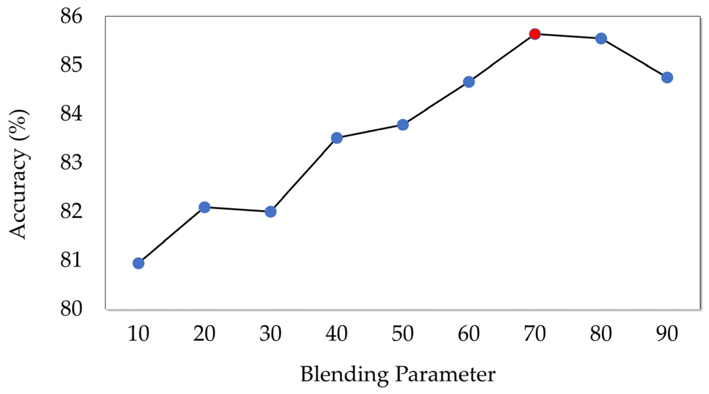In the opposite case, almost all the samples had the same transformation and were weighted equally [29]. Using this information, the EK-stars was tested using different blending parameter values from 10 to 90 when Naive Bayes was used in the pagging phase. Figure 5 shows the change in the classification accuracy for each value. It is apparent that there was an enhancement in the performance until the blending parameter was selected as 70 (the best value, 85.64% accuracy). After that, the accuracy decreased. Therefore, the EK-stars was implemented using 70 as the blending parameter.

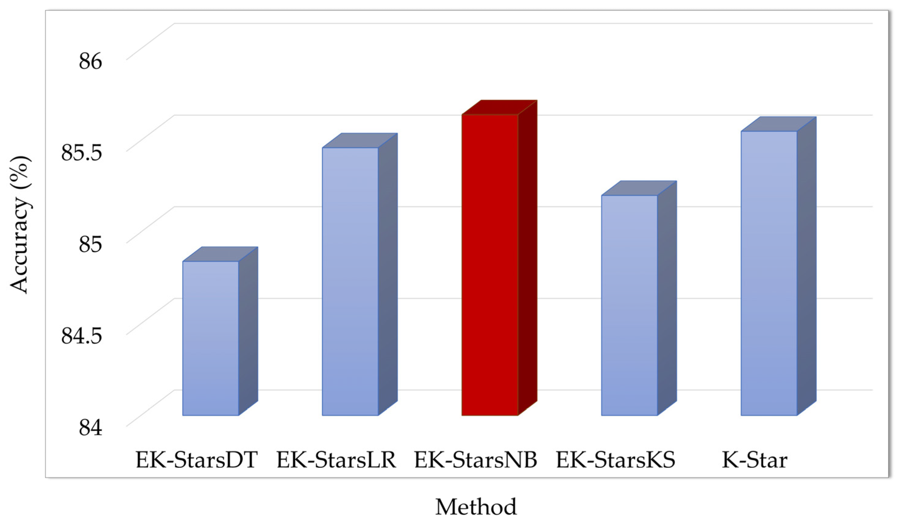
The strong instances determined by the classification probabilities were more likely to be selected in the pagging step of the EK-stars. These probabilities were obtained by applying different methods. In this study, the naive Bayes (NB), logistic regression (LR), decision tree (DT), and K-star (KS) classifiers were separately applied with their default parameters in the Weka library to identify the classification probabilities of the instances. Figure 6 displays these experimental results based on the accuracy when the blending parameter was 70. The EK-stars was named from the method used in the pagging step. For example, the EK-stars using NB as the probabilistic method was depicted as EK-starsNB. According to the results, EK-starsNB predicted the next-day rainfall status more accurately than the others with an accuracy of 85.64%. The accuracy (85.55%) of the original K-star classifier was also compared to the EK-stars, although there was not a very remarkable variation. An improvement in the performance was observed when EK-starsNB was applied.

Apart from the accuracy metric, the other performance measures were also considered to analyze the results from different perspectives. For this purpose, weighted averages of the recall, precision and f-score measures, and Cohen’s kappa coefficient were also measured and the considered findings are shown in

Table 4. Evaluation of the applied methods under the other performance metrics when the blending parameter was 70.

Method	Recall	Precision	F-Score	Kappa Coef.
K-star	0.855	0.844	0.844	0.483
EK-starsLR	0.855	0.843	0.842	0.475
EK-starsDT	0.848	0.836	0.838	0.468
EK-starsKS	0.852	0.840	0.839	0.468
EK-starsNB	0.856	0.845	0.844	0.485

. The recall presents the information on how many samples with a real positive class are predicted as positive. Nevertheless, it does not give any information about the prediction quality on the negative class. The precision gives the information on how many of the samples predicted in the positive class are actually positive. Separately, the recall and precision metrics can be useless. If a classifier always predicts the positive class, the recall will be high. On the contrary, if the model never predicts the positive class, the precision will be high. Their results cannot be reliable in such cases. The f-score can be a good solution to this problem by taking the harmonic average of the recall and precision. Table 4 shows that there was no significant difference among the results of the applied methods from considering the weighted averages of the recall (around 0.85), precision (around 0.84), and f-score values (around 0.84). In addition to the classification accuracy, these metrics also proved that the EK-stars had a considerably high prediction capability.

The kappa statistic is a measure of how closely the samples classified by a machine learning classifier match the data labeled as the ground truth by comparing it to the expected accuracy of a random classifier. That means it considers random chance. According to the study in [30], the value of the kappa coefficient was interpreted in the interval < 0.00 as poor, 0.00–0.20 as slight, 0.21–0.40 as fair, 0.41–0.60 as moderate, 0.61–0.80 as substantial, and 0.81–1.00 as almost perfect. According to the results in Table 4, all the applied methods obtained a moderate agreement (around 0.470) in terms of the kappa statistic. Although the results were very close to each other, the EK-starsNB was ahead of the others by a fractional difference.

Another study was conducted on the region-based rainfall forecast. The original K-star classifier and the best-performing classifier from the previous part mentioned as EK-starsNB were compared to determine each region’s rainfall status by using the blending parameter of 70.

Table 5. Comparison of the proposed method with the original K-star classifier in terms of the classification accuracy while predicting the rainfall for the different locations.

Location	Accuracy (%)
	K-star	EK-stars
Alice Springs	91.11	91.11
Brisbane	75.44	73.68
Cairns	75.56	80.00
Canberra	81.82	81.82
Cobar	90.91	90.91
Coffs Harbour	75.00	75.00
Darwin	73.77	77.05
Hobart	88.10	88.10
Melbourne	78.38	72.97
Melbourne Airport	80.36	82.14
Mildura	83.02	83.02
Moree	86.49	89.19
Mount Gambier	71.11	75.56
Norfolk Island	73.47	71.43
Nuriootpa	78.26	78.26
Perth	91.04	88.06
Perth Airport	90.16	86.89
Portland	62.86	71.43
Sale	79.41	82.35
Sydney	88.57	88.57
Sydney Airport	73.21	78.57
Townsville	92.50	92.50
Wagga Wagga	82.35	86.27
Watsonia	75.44	75.44
Williamtown	76.00	76.00
Woomera	92.11	92.11
Avg.	81.02	81.86

demonstrates the classification accuracies of both methods for the different locations. EK-starsNB performed better or with an equal accuracy in 21 out of the 26 regions. In some regions, for example in Portland, EK-starsNB increased the accuracy to a large extent (from 62.86% to 71.43%). Considering the average classification accuracies of all the regions, EK-starsNB outperformed the K-star with an 81.86% accuracy.

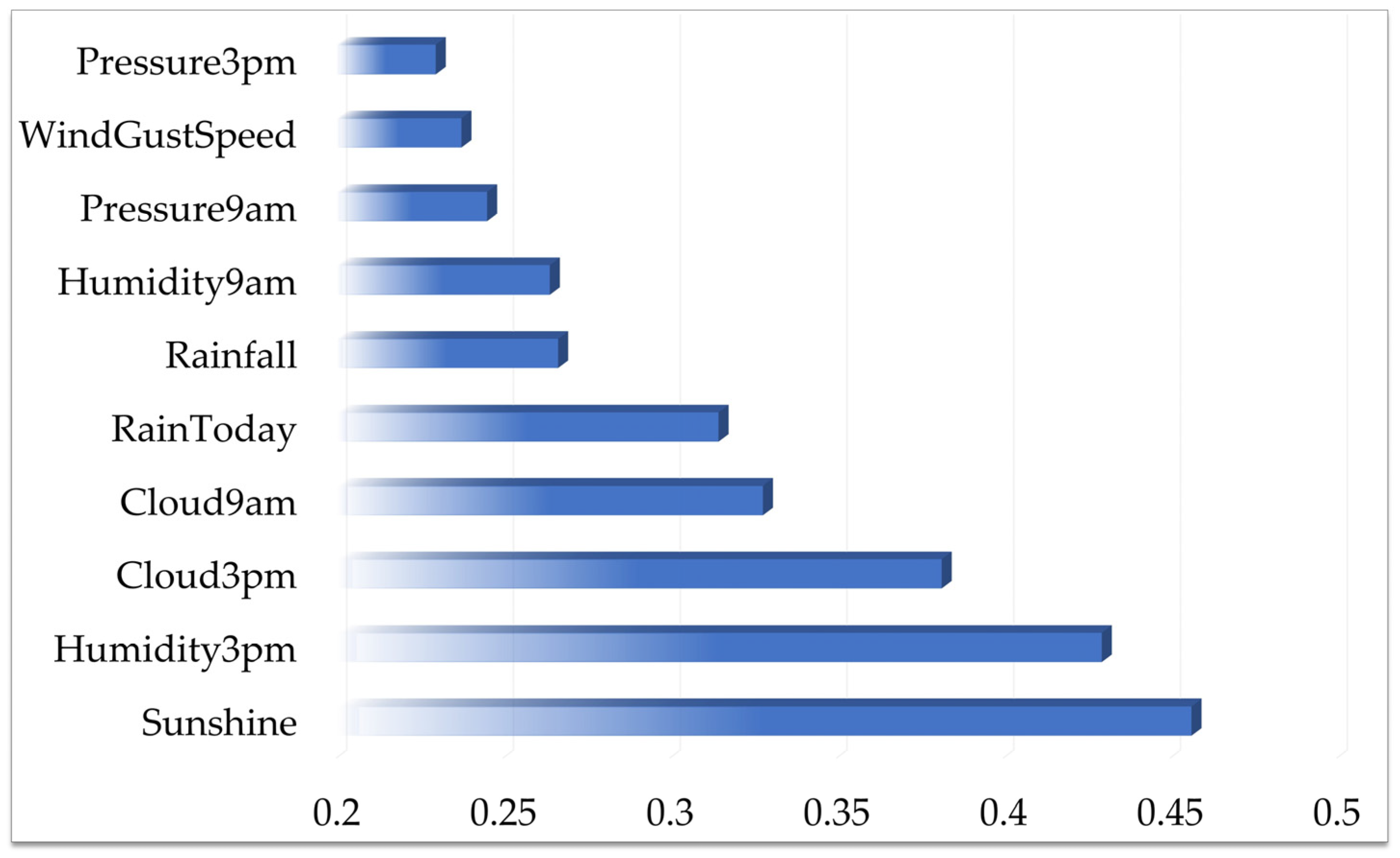
The selection of the important features increased the accuracy of the classifiers in many cases. In this direction, the most important ten features were determined for further evaluation in the experiments. For this purpose, Pearson’s correlation technique was used to determine the relationship between the features and the class attribute. These selected attributes were Sunshine, Humidity3pm, Cloud3pm, Cloud9am, RainToday, Rainfall, Humidity9am, Pressure9am, WindGustSpeed, and Pressure3pm. Figure 7 displays the worth of each attribute (0.2297 to 0.4563) by measuring the Pearson’s correlation values between the target attribute “RainTomorrow”. Sunshine was the most relevant feature since the radiation from the Sun would be directly related to a less or more cloudy day. Therefore, there would be a lower or higher probability of rain. Humidity was the second most correlated variable since the higher the humidity, the greater the possibility of rain. A high correlation with cloudiness was reasonable since the greater the number of clouds, the more likely it would rain. Rainfall was a feature that indicated the rain that had fallen (in mm), so it was an important measure that indicated whether it would rain tomorrow.

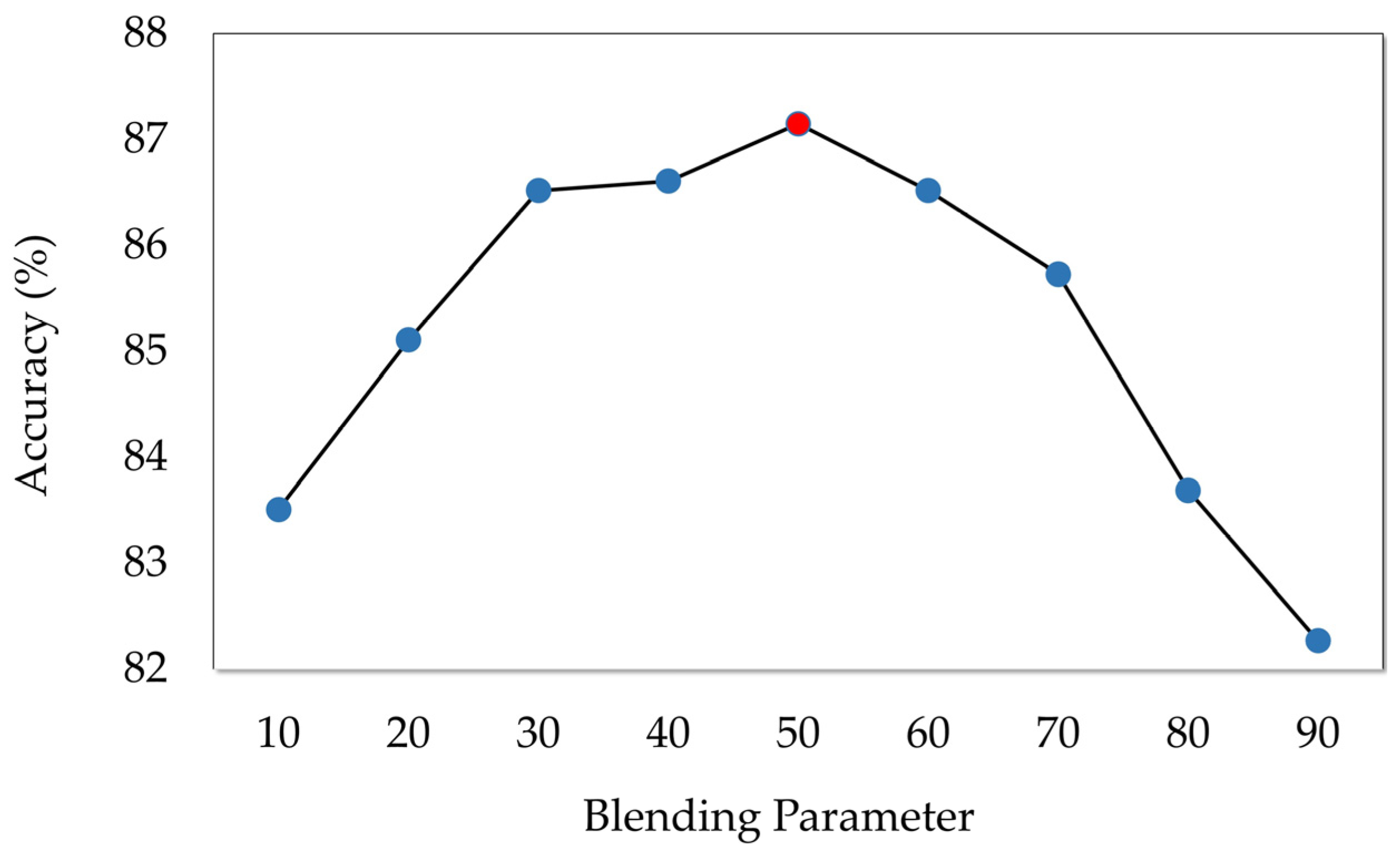
The experiment to select the best blending parameter was repeated on the data after the feature selection was applied. Since the most accurate predictions were achieved using logistic regression in the pagging phase of the EK-stars, logistic regression was used in the experiments. Figure 8 shows the changing trend of the classification accuracy using the blending parameters from 10 to 90. It was a bell-shaped curve. The worst performance was 82.57% when 90 was selected as the blending parameter, and the best was 87.15% when the value was 50. The general accuracy also increased from 85.64% to 87.15% after the selection of the significant features.

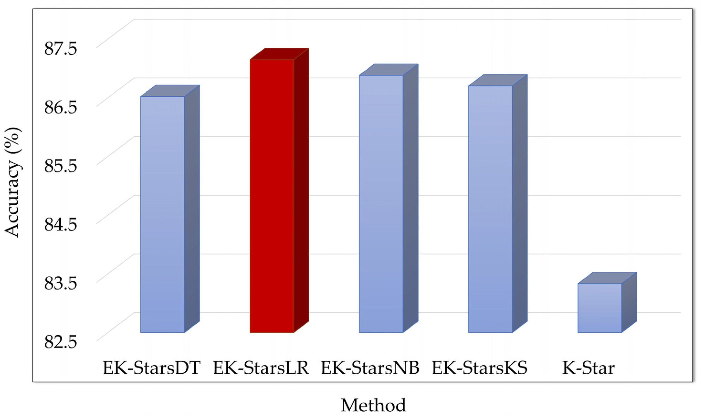
The performance of the EK-stars was monitored by applying four different methods in pagging after the feature selection, using 50 as the blending parameter. The original K-star was also implemented using the same blending parameter of 50 without the feature selection. Then, it was compared to our method to show the effect of using both the feature selection and the proposed method on the classification accuracy. Before the feature selection, the predictions of EK-starsNB were the most accurate with an 85.64% accuracy compared to the others. However, EK-starsLR outperformed EK-starsNB and obtained the best classification accuracy of 87.15%. The original K-star without the feature selection fell behind all the EK-stars variations with an accuracy of 83.33%. As shown in Figure 9, the feature selection enhanced the performance.

The other performance metrics (such as Cohen’s kappa coefficient and the weighted averages of the recall, precision, and f-score) were also evaluated after the feature selection using the optimum value (50) of the blending parameter, as given in

Table 6. Evaluation of the applied methods under the other performance metrics after the feature selection was applied using the blending parameter of 50.

Method	Recall	Precision	F-Score	Kappa Coef.
K-star	0.833	0.825	0.828	0.449
EK-starsLR	0.871	0.866	0.858	0.524
EK-starsDT	0.865	0.857	0.851	0.502
EK-starsKS	0.867	0.862	0.850	0.497
EK-starsNB	0.869	0.862	0.855	0.515

. Compared to the results in Table 4, the performance of the EK-stars algorithms in terms of the mentioned metrics increased when the feature selection was applied. For example, the weighted recall value of EK-starsDT increased from 0.848 to 0.865. The kappa statistics still produced values in the moderate range. However, their strength increased (for example it was updated from 0.475 to 0.524 for EK-starsLR). It was apparent that the K-star fell behind all the EK-stars methods for each metric while EK-starsLR performed the best compared to the others. The results of the different metrics proved that the EK-stars algorithms outperformed the traditional K-star classifier.

A region-wide analysis was repeated using EK-starsLR as the predictor on the data after the feature selection was applied. The accuracies obtained by the original K-star applied using the blending parameter of 50 on the data without the feature selection were also compared to the accuracies obtained by EK-starsLR. In the majority of the regions (17 out of 26) shown in

Table 7. Comparison of the proposed method with the original K-star classifier in terms of the classification accuracy while predicting the rainfall for the different locations after the feature selection was applied.

Location	Accuracy (%)
	K-star	EK-stars
Alice Springs	91.11	91.11
Brisbane	78.95	70.18
Cairns	73.33	86.67
Canberra	81.82	68.18
Cobar	90.91	81.82
Coffs Harbour	75.00	83.33
Darwin	72.13	78.69
Hobart	88.10	85.71
Melbourne	72.97	81.08
Melbourne Airport	82.14	83.93
Mildura	83.02	84.91
Moree	89.19	91.89
Mount Gambier	68.89	75.56
Norfolk Island	71.43	75.51
Nuriootpa	76.09	80.43
Perth	89.55	83.58
Perth Airport	88.52	88.52
Portland	74.29	77.14
Sale	76.47	70.59
Sydney	88.57	91.43
Sydney Airport	71.43	85.71
Townsville	90.00	92.50
Wagga Wagga	82.35	84.31
Watsonia	68.42	77.19
Williamtown	72.00	72.00
Woomera	92.11	92.11
Avg.	80.34	82.08

, EK-starsLR performed the best in terms of the accuracy. Additionally, it succeeded in the same performance with the original K-star in three out of the 26 locations. Performing the feature selection significantly increased the accuracy in a number of cities compared to the case without the feature selection. For example, in the city of Coffs Harbour, the accuracy escalated from 75% to 83.33%. When the average accuracy of all the cities was taken into consideration, the general performance was positively changed on behalf of EK-starsLR, which increased from 81.86% to 82.08%. On the other side, the original K-star obtained an 80.34% accuracy, and it could not predict the rainfall status as well as EK-starsLR.

In the final step, the literature studies that took the same subject as the main aim and used the same dataset were investigated and compared to our study.

Table 8. Comparison of the proposed method with the state-of-the-art studies in the literature.

Reference	Year	Method	Split Ratio	Accuracy (%)	Recall	Precision	F-Score	Kappa Coef.
Sarasa-Cabezuelo [31]	2022	NN	75:25	84.00	0.530	0.650	0.590	0.490
		DT		83.00	0.460	0.610	0.520	0.420
		RF		83.00	0.660	0.570	0.610	0.500
		KNN		83.00	0.320	0.700	0.440	0.360
Proposed Method		EK-stars		85.60	0.856	0.849	0.838	0.472
Zhao et al. [32]	2022	LR	80:20	85.00	-	-	-	-
		DT		78.00
		LSTM		85.00
		AdaBoost		82.00
		Bagging		79.80
		KNN		80.00
Proposed Method		EK-stars		87.15	0.871	0.866	0.858	0.524
Ahmad [33]	2022	KNN	80:20	85.00	0.480	0.672	0.560	-
		CART		80.19	0.200	0.560	0.300	-
Proposed Method		EK-stars		87.15	0.871	0.866	0.858	0.524
Mahadware et al. [34]	2022	CatBoost	70:30	81.37	-	-	-	-
		Perceptron		77.60
Proposed Method		EK-stars		85.05	0.850	0.844	0.831	0.465
Dieber and Kirrane [35]	2022	DT	70:30	79.00	0.790	0.830	0.800	-
		RF		80.00	0.800	0.830	0.810	-
		LR		79.00	0.790	0.840	0.800	-
		XGBoost		85.00	0.850	0.850	0.840	-
Proposed Method		EK-stars		85.05	0.850	0.844	0.831	0.465
Baharisangari et al. [36]	2022	DT	80:20	76.14	-	-	-	-
		KNN		81.04
		SVM		82.61
		ANN		84.73
		w-GSTL-NN		81.69
Proposed Method		EK-stars		87.15	0.871	0.866	0.858	0.524
Deng [42]	2020	LR	70:30	84.95	-	-	-	-
		DT		83.32
Proposed Method		EK-stars		85.05	0.850	0.844	0.831	0.465
Liu et al. [43]	2020	AdaBoost	80:20	84.70	-	-	0.614	-
		LogitBoost		83.94			0.546
		GentleBoost		84.19			0.581
		Rboost		84.39			0.567
		CB-AdaBoost		84.39			0.567
		Gradient Boosting		84.07			0.517
		SSAdaBoost		84.77			0.629
		SSGB		84.23			0.560
Proposed Method		EK-stars		87.15	0.871	0.866	0.858	0.524
Oswal [44]	2019	RF	75:25	84.38	-	-	-	-
		Gradient Boosting		84.45
		LR		83.71
		AdaBoost		84.90
		KNN		85.04
		DT		83.06
Proposed Method		EK-stars		85.60	0.856	0.849	0.838	0.472

displays the accuracies obtained in these studies and the results of our method. The comparisons were made by applying the optimum model EK-starsLR with the blending parameter of 50, which will be mentioned as EK-stars in short. In the study [31], various machine learning methods, including the KNN, DT, RF, and NN were performed, and parameter tuning was applied to determine the optimum values of the parameters. The best accuracy was obtained using NN at 84% when the ratio of 75–25 was used as the training and test split. In order to make a valid comparison, the EK-stars algorithm was also trained using a 75–25 split ratio. According to the results, the EK-stars obtained a 85.60% accuracy and outperformed the NN. In addition, the kappa coefficient and the weighted averages of the precision, recall, and f-score values were also analyzed. Even though the kappa coefficient with the value of 0.5 was higher than ours (0.472) when the RF was applied, the results of the other metrics were obtained using EK-stars with the highest precision (0.849), recall (0.856), and f-score (0.838) values. In another study [32], the KNN, DT, and LR were implemented using the meteorological data, and the LSTM was also applied to analyze the effect of the previous weather of the week on the rainfall data. Two ensemble learning methods, bagging and adaptive boosting (AdaBoost), were also performed. The best-performing predictor was identified as the LR with an 85% accuracy when an 80 to 20 training and test split was used. However, the LR did not manage to obtain better results than the EK-stars. The CART, SVM, and KNN were the predictors in the study [33], and they were applied on both the processed data, where the data preprocessing and feature selection were performed, and the original dataset when the ratio of the training and test split was 80 to 20. The KNN was the most accurate method using the original dataset with a value of 85%. Our proposed method correctly classified more samples compared to the results of this study in terms of the accuracy. Furthermore, other analyses were also conducted on the weighted averages of the precision, recall, and f-score. The best model (KNN) in the mentioned study resulted in values of 0.672, 0.480, and 0.560 for the precision, recall, and f-score, respectively. On the other side, the EK-stars performed very well and showed a considerable difference compared to the KNN by obtaining 0.866, 0.871, and 0.858 for these same measures. In [34], after several feature engineering steps were practiced on the dataset, the categorical boosting (CatBoost) and perceptron methods were performed, and at most, an 81% accuracy was obtained, which was lower than the EK-stars. Dieber and Kirrane [35] applied four models (DT, RF, LR, and XGBoost) using a 70 to 30 ratio for the training and test set under their proposed framework that was designed for an easy interpretation of the experimental outputs. The XGBoost achieved the best accuracy compared to the others. In this direction, the EK-stars was implemented using a 70–30 ratio and obtained an 85.05% accuracy. The weighted averages of the precision, recall, and f-score metrics were also conducted, and it was shown that our method and the XGBoost gave similar results of approximately 0.850 for all the metrics. The study in [36] presented a method based on neural networks to learn spatiotemporal knowledge in the form of weighted graph-based signal temporal logic (w-GSTL-NN) formulas. The experiments were conducted on 20% of the whole dataset. Their proposed method could not achieve the most accurate results compared to the other applied models and our model EK-stars, which obtained an 81.69% accuracy. The sequential ANN model and SVM were found to be better for obtaining the accuracy values, with approximately 85% and 83%, respectively. Umamaheswari and Ramaswamy [37] proposed a novel methodology using both preprocessing (the moving average probabilistic regression filtering (MV-PRF)) and optimization techniques (the time variant particle swarm optimization (TVPSO)). Then, neural network methods such as back propagation neural networks (BPNN), iterative convolutional neural networks (ICNN), and deep convolutional neural networks (DCNN)) were applied. The DCNNs classified the test samples better than the others with nearly an 80% accuracy. However, they didn’t state the training test split ratio, so it was meaningless to compare it to our results. The different optimization algorithms of the neural networks, such as the adaptive moment estimation (Adam), an extension of the Adam optimizer (Adamax), adaptive gradient (Adagrad), Nesterov-accelerated Adam (Nadam), stochastic gradient descent (SGD), and root mean square propagation (RMSProp), were analyzed in the study of Pilošta [38]. They achieved accuracy values very close to each other (approximately 85%). The test set ratio was missing in this study too. By including and applying the Moon’s phases as a new feature to the original rainfall dataset, the predictions were made by the LR and RF in the study [39]. The best accuracy was mentioned as 86% by the RF. The ratio of the training and test split was not stated. He [40] used pool-based active learning to forecast the rainfall status and compared its results with the random sampling using the logistic regression model. It was reported that they had almost the same prediction accuracy (82%). They did not clearly state the training and test set ratios. In [41], the rain prediction was performed to obtain an opinion on a probable wildfire, so a system based on the RF was developed. They obtained 84.70% classification accuracy but did not comment on which setup was used in the training/test set. Deng [42] used the LR and DT with a 70 to 30 training and test split, and the LR outperformed DT in the experiments. A new sample selection framework (self-sampling (SS)) for the boosting algorithms was proposed in [43]. Several boosting algorithms, including the logistic boosting (LogitBoost), Gentle AdaBoost (GentleBoost), robust boosting (RBoost), conditional risk-based AdaBoost (CB-AdaBoost), and self-sampling gradient boosting (SSGB), were practiced. One of their proposed models (self-sampling AdaBoost (SSAdaBoost)) obtained the most accurate rainfall predictions compared to the others. Moreover, the weighted average of the f-score metric was also measured and the SSAdaBoost achieved 0.629 as the best predictor. The EK-stars outperformed the SSAdaBoost in terms of the f-score with a value of 0.858. In [44], the feature selection and resampling (undersampling and oversampling) techniques were implemented on the dataset. The LR, DT, KNN, RF, AdaBoost, and gradient boosting were used in the experiments. Approximately an 85% accuracy was obtained by the KNN using the original data when the ratio of the training and test split was 75 to 25 and a stratified 10-fold approach was used. In summary, the neural network models or ensemble learning strategies were generally preferred in the mentioned studies due to their predictive power.

As shown in Table 8, the proposed EK-stars method outperformed the recent studies in three scenarios based on the different training/test split ratios. When the 70:30 split ratio was applied, the average accuracy of the studies [28,29,36] was 81.28% while the EK-stars achieved an 85.05% accuracy. In the experiments with the 75:25 ratio, the studies in [25,38] were performed with an accuracy of 83.85% on average while the EK-stars concluded with 85.60%. Finally, when tested with the 80:20 split ratio, the average accuracy of the mentioned methods [26,27,30,37] was 82.66% compared to 87.15% in the EK-stars. The improvements made by the EK-stars were approximately 4%, 2%, and 4.5%, respectively. As the training data increased, the success rate of the EK-stars increased accordingly, which was reasonable because the number of samples representing each class was increased. To make a general conclusion, the average classification accuracy for all the mentioned studies and the average accuracy of the EK-stars were obtained by taking their mean. As a result, the proposed EK-stars method performed the best on average compared to the recent studies (82.68%) in terms of the classification accuracy with a value of 85.93%. Thus, our method demonstrated its superiority over the others with an over 3% improvement on average by utilizing the power of a new ensemble learning strategy. Furthermore, the results of the other performance metrics (recall, precision, f-score, and kappa coefficient) proved that the EK-stars managed to produce satisfactory and reliable predictions.

6. Conclusions and Future Work

The estimation of rainfall, which is one of the crucial issues in the environmental field, was handled using a machine learning approach in this study. Ten years of historical data consisting of the temperature, pressure, sunshine, humidity, wind direction, etc. collected in the regions of Australia were used to predict the next-day rainfall status. An approach abbreviated as the EK-stars, which was based on ensemble learning, was presented for this aim. The general mechanism of this method was that a number of K-star classifiers were performed in each ensemble iteration by randomly selecting the strong instances using a probabilistic technique. Three different scenarios were considered in the experimental study. The determination of the optimal value of the blending parameter for the K-star classifier, implementing the EK-stars with different methods, including the DT, LR, NB, and K-star in the pagging step, and applying the feature selection were carried out to obtain the best classification accuracy. Furthermore, the weighted averages of the precision, recall, f-score, and Cohen’s kappa coefficient values were also analyzed.

The main findings of this study can be summarized as follows.

▪

The EK-stars method (87.15%) achieved a higher classification accuracy than the standard K-star method (83.33%) on the same dataset.

▪

The best accuracy was obtained by the EK-stars with the logistic regression technique as the base learner.

▪

The performance of the model was evaluated using the different hyperparameter values and achieved the highest accuracy with the blending parameter of 50.

▪

When the significance of the features was investigated by the Pearson’s correlation technique, it was revealed that sunshine had the highest score. It was followed by the humidity and cloud variables.

▪

Our method (85.93%) outperformed the state-of-the-art methods (82.68%) on average. Therefore, the proposed method demonstrated its superiority over the previously reported methods [30,31,32,33,34,35,41,42,43], with an improvement of over 3%.

This study mainly contributed to the following subjects.

• The areas that will be badly affected by drought can be predicted using the proposed system. Agricultural activities in these locations continue to operate regularly using appropriate irrigation systems according to the recommendations based on the prediction results.
• When the prediction system based on the EK-stars is put into practice, it can provide an early warning alarm in case of possible flooding, and inform the authorized persons about the situation, thus enabling the necessary measures to be taken in advance.

One of the limitations of this study was the lack of an application development. Future work can include the development of an application based on the EK-stars approach that runs on the dataset, the periodic insertion of new transactional data in a storage system, and the automatic updating of the model over time. In this way, the designers and decision-makers can benefit from the predictions of the machine learning model for sustainable development. Another limitation of this study was that it did not focus on the seasonal changes. In the future, this study can be extended to either investigate the seasonal changes of rainfall in different locations or perform and test the EK-stars in different fields of expertise.