Article

Prioritization of Off-Grid Hybrid Renewable Energy Systems for Residential Communities in China Considering Public Participation with Basic Uncertain Linguistic Information

School of Advanced Interdisciplinary Studies, Hunan University of Technology and Business, Changsha 410205, China
*
Author to whom correspondence should be addressed.
Sustainability 2023, 15(11), 8454; https://doi.org/10.3390/su15118454
Submission received: 4 April 2023 / Revised: 15 May 2023 / Accepted: 18 May 2023 / Published: 23 May 2023
(This article belongs to the Special Issue Application of Information Technology (IT) for Sustainability)

Abstract

:
In recent years, the adoption of Hybrid Renewable Energy Systems (HRESs) is rapidly increasing globally due to their economic and environmental benefits. In order to ensure the smooth implementation of HRESs, it is important to systematically capture societal preferences. However, few studies focus on the effective integration of public opinion into energy planning decisions. In this study, a decision-making approach for public participation in HRES planning is proposed to optimize the configuration of off-grid HRESs. First, an HRES evaluation index system considering public participation was constructed; to address the situation where the public from different backgrounds may have limited and inconsistent understanding of indicators, the basic uncertain linguistic information (BULI) is introduced to express evaluations and associated reliability levels. The indicator weights were then determined through the evaluation of both the public and the expert opinions. Second, the BULI-EDAS decision approach was developed by extending the EDAS method to the BULI environment to optimize HRES planning. Finally, the proposed model was applied to identify the optimal configuration in rural China. The comparative analysis results show that the proposed method can avoid misunderstandings and facilitate realistic public judgments. The selected optimal plan has a standardized energy price of 0.126 USD/kWh and generates 45,305 kg CO2/year, resulting in the best overall performance. The proposed HRES planning method provides a practical approach for decision makers to conduct HRES planning in a public participation environment to promote clean energy transitions.

1. Introduction

Energy is the foundation of human survival and development. Nowadays, the world faces the challenge of ensuring energy security and sustainable development while minimizing environmental pollution. The use of renewable energy has great environmental benefits which have a vital role in achieving global climate and sustainability goals. However, many stakeholders are unwilling to invest in and participate in the renewable energy system, due to low social satisfaction [1], large area occupation [2], and high initial investment [3], which restrict the promotion of its use. The development of hybrid renewable energy systems (HRESs) is a more sensible choice for integrating multiple energy technologies to reduce the total system costs while generating benefits in all technical, economic, and environmental aspects [4]. HOMER, along with its easy-to-use operation and fast and efficient analysis results, is widely used among researchers to model HRESs [5]. However, this software can only perform single-objective optimization based on economics in the feasibility analysis of the system. To augment the level of sustainability as the paramount policy goal of the nations, energy concerns are no longer considered in isolation but rather in conjunction with multiple development challenges (e.g., economic, social, policy, and environmental) [6]. Multi-Criteria Decision Making (MCDM) approaches can tackle these challenging tasks, including contradictory criteria and different objectives in energy planning decisions.
The selection of HRES alternatives is a typical MCDM problem. Previous studies have studied it from different perspectives. The design optimization of the renewable energy system configuration in the Beijing Xiongan New Area was simulated by HOMER software to address the limitations of a single decision method; three different MCDM methods were used to determine the indicator weights and select the optimal system configuration [6]. Taking into account the ambiguity and uncertainty of evaluation information, the IVHF-ELECTRE II method for ranking renewable energy options was proposed and a case study was conducted in China [7]. Researchers have conducted technological and economic analyses of grid-connected and off-grid HRES systems and found that grid-connected HRES systems produced more CO2 [8]; therefore, more attention has been paid to the design optimization and technical analysis of implementing stand-alone HRESs. An integrated decision model was developed and applied to a design optimization analysis of 100% clean energy system scenarios in rural Pakistan to determine the best alternative for the grid and off-grid scenarios [9]. An off-grid hybrid renewable energy system using hydrogen batteries through HOMER was simulated and the results showed that the hybrid energy storage system using hydrogen batteries was the most beneficial [10]. The existing studies investigated how to select the optimal energy system solution based on MCDM from different perspectives. However, the public’s willingness was rarely considered, particularly in the problem of measuring the social acceptability of energy portfolios; simply having experts provide ratings on a single technology is insufficient, and further research is needed, particularly on the topic of public participation.
Electricity infrastructures are technical systems that need to go in tandem with the societal systems of the populations they serve [11]. However, traditional decision making makes it difficult for the government to obtain information on public opinion of such engineering issues. Additionally, the absence of public participation mechanisms often leads to a decrease in social acceptance from residents, even leading to group incidents [12]. The issue of public participation mechanisms and social acceptance of energy systems has received attention from the academic community [13]. Considering the opinions of the local public, electricity pathways through renpassGIS were simulated, and the renewable energy scenarios with the preferences of local stakeholders were obtained through AHP methods [14]. Considering the participation of stakeholders and the uncertainty in the evaluation process, a fuzzy decision model was constructed, and the experimental results proved the necessity of considering stakeholder preferences [15]. To address the different stakeholder interest needs and risk preferences, wind power coupled hydrogen energy storage (WPCHES) scenarios were ranked by the TODIM method and used to investigate the impact of the risk preferences of different stakeholders on the ranking results [16]. A multi-objective optimization model for energy investments considering public opinion was proposed using a linguistic risk preference-based approach for clustering the public and incorporating public opinion through an evidential reasoning approach [17]. Previous research focused on how to optimize the configuration of renewable energy systems by directly obtaining evaluation information from experts or the public using the MCDM approach. However, the reliability level of decision makers in the process has not received much attention. Meanwhile, the lack of background knowledge and inconsistent understanding of the options in the public participation process often lead to misleading results, and these factors may even offset the benefits of public participation in decision making. When representatives and experts from specific backgrounds are involved in the process, the level of understanding of the option should be considered.
Basic uncertain information (BUI) provides a key solution for obtaining reliability information for evaluating information [18]. The basic uncertain linguistic information (BULI) is a decision-making methodology that utilizes the renowned 2-tuple linguistic representation model [19] and takes into account the reliability of evaluative information. It inherits the benefits of the 2-tuple linguistic representation model, such as high interpretability and the avoidance of information loss, making it especially useful in complex and uncertain decision-making contexts. The BULI-based method for constructing and processing uncertain linguistic assessment information was further developed and applied in sustainable building material selection to obtain optimal sustainable building materials [20].
Through literature reviews on HRES selection [6,7,8,9,10] and public participation [11,12,13,14,15,16,17], it can be found that how the public can effectively participate in HRES planning is a new area of application for MCDM methods and is rarely reported. In particular, the issue of the reliability of evaluations made by decision makers needs to be urgently addressed. Meanwhile, relevant studies [18,19,20] have shown that BULI can effectively characterize the reliability of evaluation information and has been applied in related fields. To fill this research gap, BULI is introduced in this paper to collect decision makers’ evaluation information and corresponding reliability level in a public participation environment. Then, a BULI-EDAS method was developed to address the MCDM problems. The developed method was applied to a case study in rural China to select the optimal off-grid HRES while taking public preferences into account. This paper locates its contribution within the decision-making process of public infrastructure in a public participation environment. Through comparative analysis, it indicates that public participation and the consideration of reliability levels have a significant impact on the result of decision-making. Therefore, it is imperative to take these factors into account during the process. The output of this model lays the groundwork for future system design and parameter optimization.
The rest of this paper is organized as follows: Section 2 provides the research method’s details, including resource and load estimation and component configuration of the study area. In Section 3, a BULI-EDAS-based MCDM design optimization methodology is developed. Then, the obtained results are demonstrated and discussed in Section 4. Finally, Section 5 gives the study conclusions and suggestions for future research.

2. Geographical Feature and Assessment of Load Demand

This section will describe the study area’s geographic location, local climate conditions, load needs, and system component pricing.

2.1. Study Area

The study area of this paper is a village near Wuhai City, Mongolia Autonomous Region, China. Bayin Wusu Village, with coordinates 106.32° N, 39.67° E, is located in the northernmost part of Wuhai City. The village covers an area of 13.5 square kilometers and is 8 km long from north to south, with 1223 permanent residents and a total of 3140 people. The research area selected for this study boasts abundant natural climate resources, vast land, and policy support, providing favorable conditions for the development of renewable energy power generation. Additionally, based on past literature reviews, remote rural areas are typical application areas for renewable energy, and these areas have stable load demand, making them particularly suitable for the application of HRES.

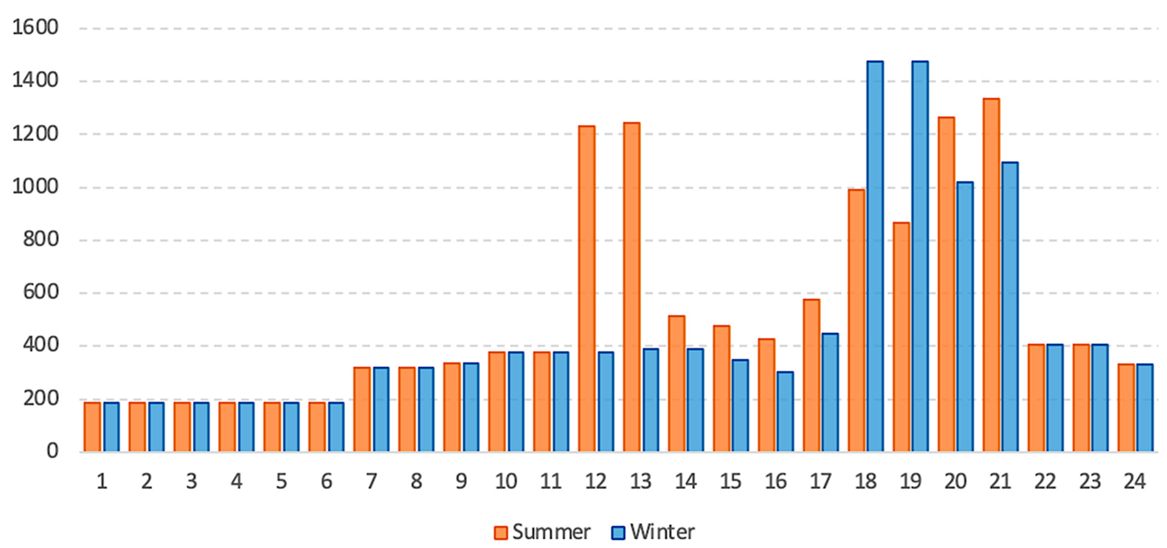
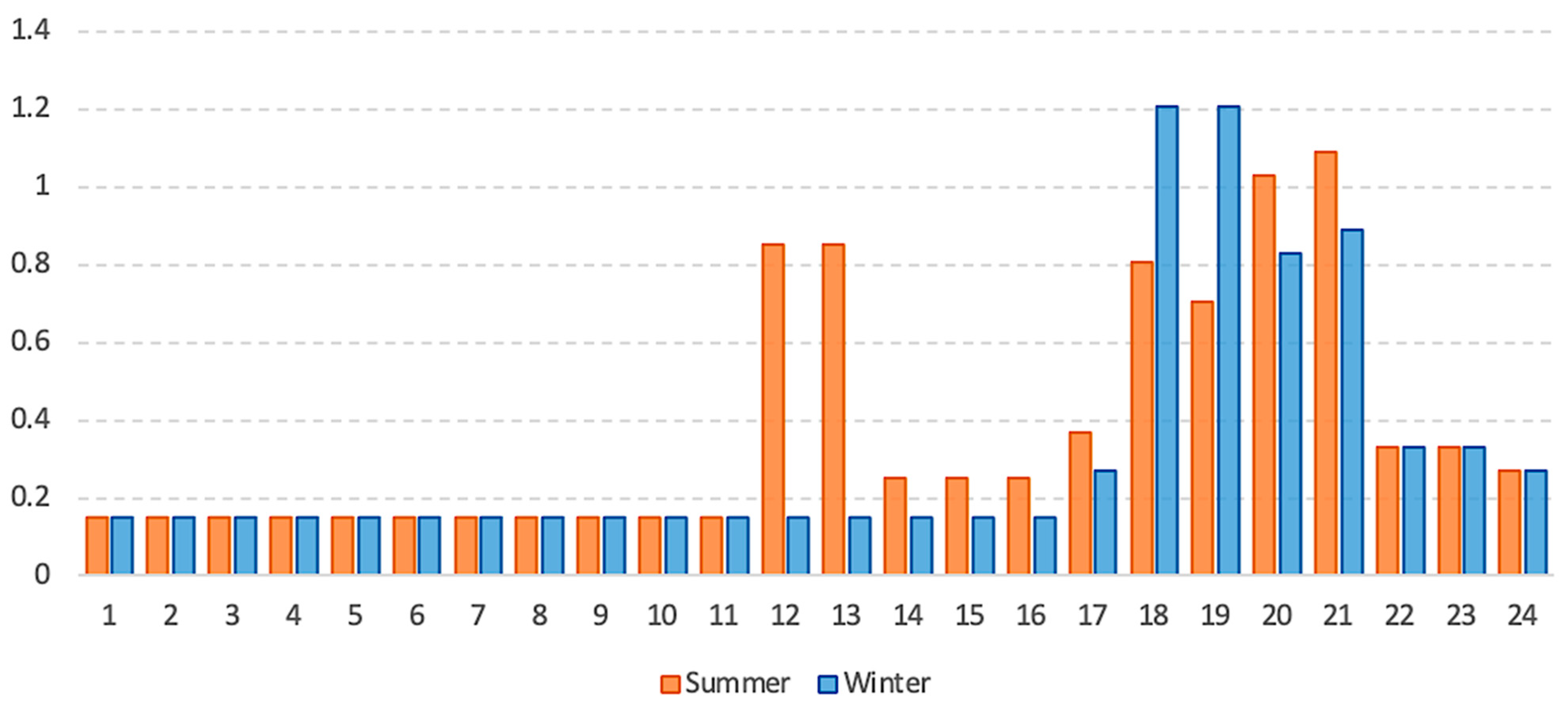
2.2. Load Estimation

The total load demand of the township was assessed mainly based on the energy requirements of the township after investigation and research. Table 1 shows the common electrical appliances used by each household and the corresponding power. We also evaluated the energy use of local agricultural cultivation, schools, hospitals, and other public facilities, and assessed the energy load data for different seasons to create realistic load curves [21] and the details are shown in Table 1 and Table 2. The average annual load demand was 12,094.67 kWh/day, with a load factor of 0.34, a peak demand of 1336.22 kWh/h in summer, and a peak demand of 1477.35 kWh/h, mainly in the evening between 18H and 21H. Two hydrogen-fueled vehicles were deployed locally, each driving 100 km per day with 80 g of hydrogen per km [22]; setting a stochasticity of 10% and 20% deviation of hours, the system required 16 kg/day of hydrogen load. Figure 1 and Figure 2 demonstrate the variation of the total load demand for a household and the township, respectively.

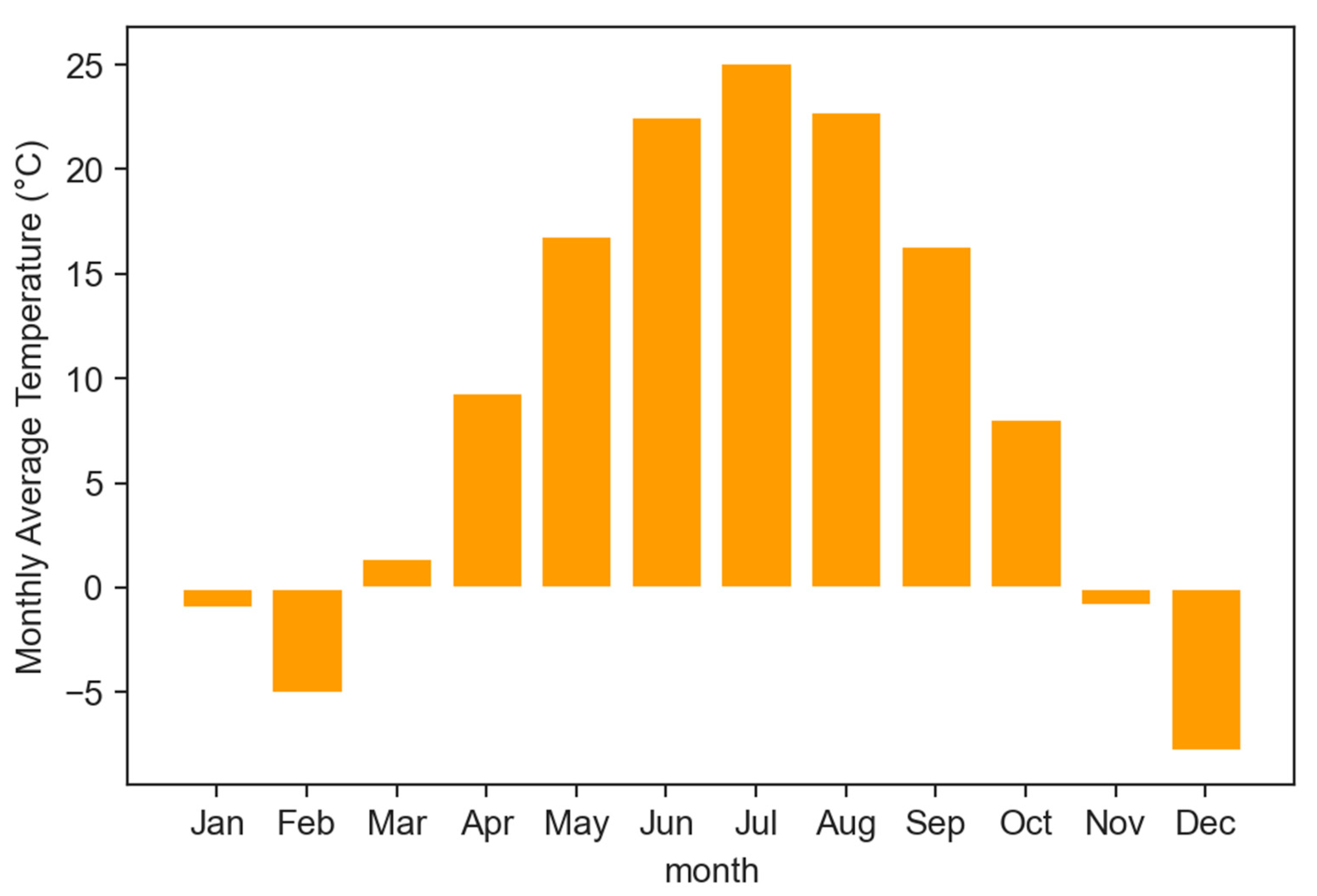
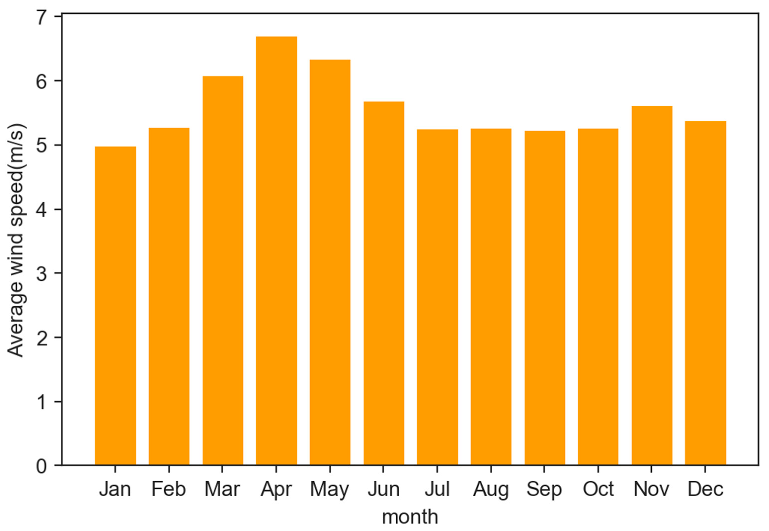
2.3. Resource Assessment

The village of Bayin Wusu, with coordinates 106.32° N, 39.67° E, has a typical temperate continental climate with an average annual temperature of 7.8–8.1 °C. Meteorological data for the study area were retrieved from the National Aeronautics and Space Administration’s Meteorology and Solar Energy Database. Figure 3 shows the local monthly average temperature; Figure 4 shows the local wind energy resources, with an average wind speed in Bayin Wusu Village of 5.6 m/s. From Figure 4 and Figure 5, we can see that the selected location has a reasonably good availability of solar irradiation and wind speed and therefore, there is great potential to develop wind energy resources here. The annual average solar radiation of Bayin Wusu Village was 4.7 kWh; Figure 5 shows the local solar radiation data and the atmospheric clearness index, and from Figure 5 we can see that the solar radiation in this place was mainly concentrated in May and June in summer and drops to the lowest level in November and December in winter, which shows that the local photovoltaic energy has strong characteristics of uneven spatial and temporal distributions. The development of HRES to improve the stability of energy production is an ideal solution.
Biomass is a promising source of energy in this region. This source is mainly assessed from the waste generated by the local population, where the average daily human excreta was estimated to be 0.350 kg [22] and the average daily kitchen waste generated per person was 0.300 kg [23]. Given the actual collection process, the resources are scattered and the collection process generates certain losses, so it is necessary to multiply the collection coefficient to obtain the actual collection volume, and finally the daily collectible biomass in the region was 1.4287 tons. Table 3 and Table 4 respectively present detailed data on the estimation of biological resources and the footprint of each component.

2.4. Component Configuration

The financial details of the different components and the corresponding technical parameters were obtained by a literature review; these details, the economic data of the components in the system, and the corresponding references can be found in Table 5. The detailed system parameters of the components can be found in Appendix C.

2.5. Global Parameter Settings

The global parameter settings of HOMER are shown in Table 6: the inflation rate is 2% which is the average value for 2000–2019 [22], and the annual discount rate is 8% [25]. The carbon emission penalty price is set to 3 USD/t, and the simulation time step is 1 h. To ensure the stability of the use of the system, the maximum annual system capacity shortage rate is set to 0%.

2.6. Control Strategies

The HOMER software has different load control strategies built in: load following and cyclic charging strategies. In the load following strategy, the generator works only in emergency situations to meet the load demand, and other lower priority load demands (e.g., battery charging) are allocated to renewable energy sources. In the cyclic charging strategy, generators are used for both on-demand power supply and battery charging. Considering the stochastic nature of renewable energy generation and load demand, the load following strategy (LFS) was used as the control strategy of the HRES system in this study.

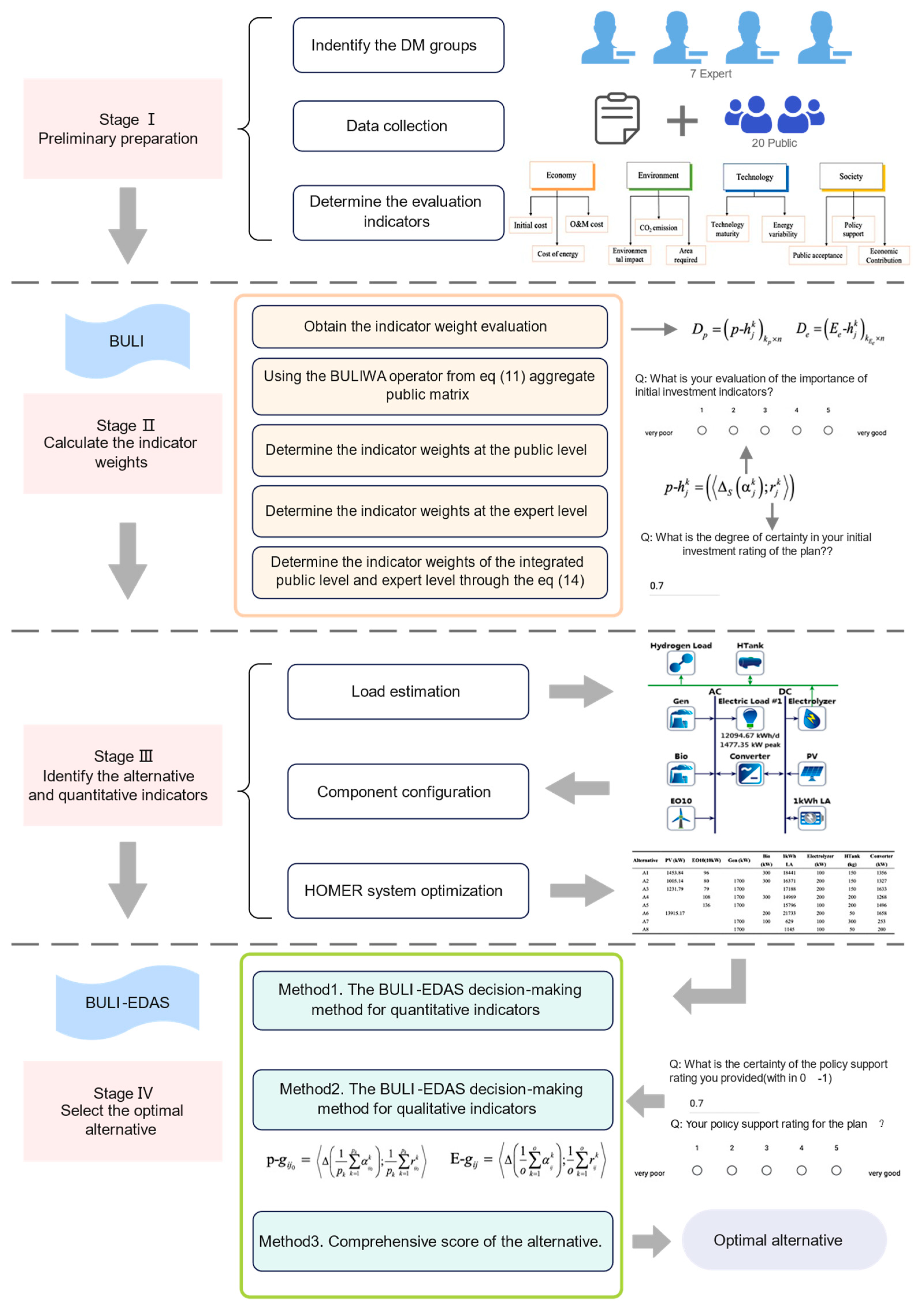
3. Optimization Method

The HRES selection method proposed in this study was primarily divided into four stages, as illustrated in Figure 6. A detailed explanation of the steps is provided below.
(1) Stage I involved the preliminary preparation, including the identification of decision makers, data collection on local resources, and establishment of evaluation indicators for HRES decision making. (2) In Stage II, indicator weights were calculated by collecting evaluation information and corresponding reliability through questionnaires in the public BULI environment. The variable Δ s α j k was collected through a 5-granularities Likert scale in the questionnaire, while the variable r j k was collected through corresponding reliability questions in the questionnaire. The empirical and model variable correspondence can be seen in Figure 6. Evaluation information was also collected from experts and aggregated to obtain expert-level indicator weights. Finally, the weights from both levels were combined to obtain the comprehensive indicator system weights. The details can be found in Section 3.3.1. (3) Stage III involved the identification of alternatives and quantitative indicators. The HOMER Pro microgrid analysis tool was used to determine feasible solutions and obtain quantitative indicator information. This involved load estimation based on environmental data, system modeling and inputting configuration data, and obtaining feasible solutions and quantitative data through HOMER simulation optimization. (4) In the final stage, the decision method of BULI-EDAS was constructed, which combined qualitative and quantitative data and considered public and expert opinions to calculate the optimal HRES plan. The detailed process is shown in Section 3.3.2.

3.1. Preliminary and Problem Description

In this subsection, a novel algorithm for selecting the optimal alternative is developed. Let A = { A i | i = 1 , 2 , , m } be an alternative set, Q = Q j | j = 1 , 2 , , n where n evaluating criteria set for A , and W = { w i | i = 1 , 2 , N } is the weighting vector with conditions w j [ 0 , 1 ] and j = 1 n w j = 1 for the criteria set.
The evaluation indicator system is divided into qualitative and quantitative indicators; therefore, the evaluation criteria set Q is divided into the quantitative index Q 1 and qualitative index Q 2 , where
Quantitative indicators: Q 1 = Q 1 j | j = 1 , 2 , , j Q 1 = Q 1 , Q 2 , , Q 5 ;
Qualitative indicators: Q 2 = Q 2 j | j = 1 , 2 , , j Q 2 = Q 7 , Q 9 , , Q 11 ;
This research utilized a questionnaire to collect evaluative data, and the expert group E = E k | k = 1 , 2 , , o consists of experts in the field of energy technology, government staff, and energy investors. Considering the public’s opinion, N citizens were selected to form a public representative group in energy system planning. Experts or the representative group provided evaluation information through the following linguistic set.
S = S i | i = 0 , 1 , , 4 = v e r y   p o o r ,   p o o r ,   f a i r ,   g o o d ,   v e r y   g o o d
Given that decision makers from different backgrounds may have limited and inconsistent knowledge of the indicators, each evaluation question was attached to a reliability score r ( 0 , 1 ) .

3.2. Basic Uncertain Linguistic Information (BULI)

When representatives and experts from different backgrounds are involved, the level of understanding of the option should be considered. Basic uncertain information (BUI) provides a key solution for obtaining reliability information for evaluating information. The related concepts of basic uncertain information (BUI) and BULI are described in this section.
Definition 1 [29].
Let  S = { s 0 , s 1 , , s 4 }  be an LTS and  S ¯  the 2-tuple set associated with   S  defined as  S ¯ = S × [ 0.5 , 0.5 ) . Let  α [ 0 , τ ]  be a value representing the result of a symbolic aggregation operation. The 2-tuple that expresses the equivalent information to  α  is then obtained as:
Δ S : [ 0 , τ ] S × [ 0.5 , 0.5 ) ,
where
Δ S ( α ) = ( s i , Ψ ) ,   with   s i , ψ i , i = r o u n d ( α ) Ψ [ 0.5 , 0.5 )
Definition 2 [29].
Let  ( s k , α )  and  ( s l , γ )  be 2-tuple linguistic term. Then:
  • if  k < l , then  ( s k , α )  is smaller than  ( s l , γ ) ;
  • if   α = γ , then
    (a)
    if  α = γ , then   ( s k , α )   and   ( s l , γ )   represent the same information;
    (b)
    if  α < γ , then  ( s k , α )  is smaller then  ( s l , γ ) .
Definition 3 [20].
Let  S = { s α | α = 0 , 1 , , τ }   be an LTS. The pair   b j = Δ s ( α i ) ; r i , which binarily includes a 2-tuple linguistic term   Δ S ( α i )   defined on  S ¯  and its source reliability  r i 0 , 1 is called a representation of basic uncertain linguistic information (BULI).
Definition 4 [20].
Let  b i = Δ S ( α i ) ; r i   and   b j = Δ S ( α j ) ; r j  be two arbitrary BULI pairs; the comparison laws between them can be defined by
(1)
b i > b j ( α i r i > α j r j ) ( ( α i r i = α j r j ) ( α i > α j ) ) ;
(2)
b i < b j ( α i r i < α j r j ) ( ( α i r i = α j r j ) ( α i < α j ) ) ;
(3)
b i = b j ( α i = α j ) ( r i = r j ) ;
Definition 5 [20].
Let  D = { d n = Δ s ( α n ) ; r n | Δ s ( α n ) S ¯ , r n [ 0 , 1 ] . n = 1 , 2 , , N }  be the set of BULI pairs to be aggregated, in which  S  refers to a given LTS. The weighting vector is denoted by  W = { w i | i = 1 , 2 , N }  with two fundamental conditions   w n [ 0 , 1 ]  and  n = 1 N w n = 1  satisfied. Then, the elements in   D  can be aggregated by the BULI weighted averaging (BULIWA) operator, which is a mapping function.   B U L I W A : ( D ( S ¯ ) ) n D ( S ¯ )  can be defined as follows:
B U L I W A Δ S ( α 1 ) ; r i , , Δ S ( α N ) ; r N = Δ n = 1 N w n α n ; n = 1 N w n r n ;

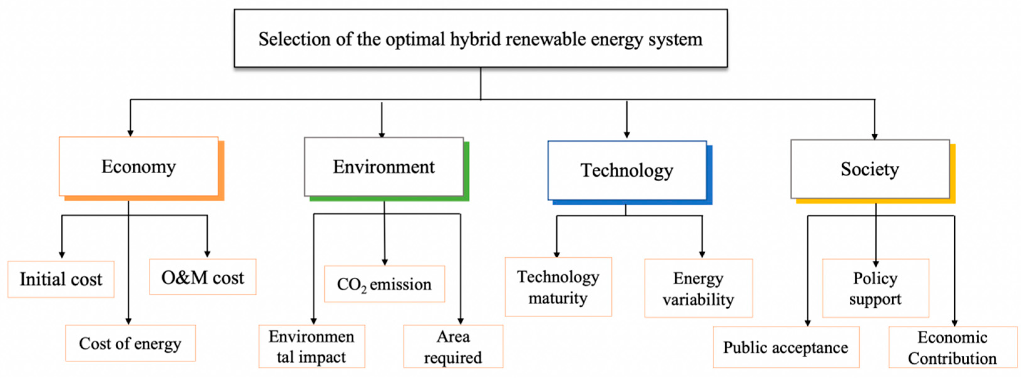
3.3. Indicator System

Based on HOMER PRO software, this study analyzed the feasibility and configuration of off-grid energy solutions based on wind, photovoltaic, bioenergy, hydrogen, and energy storage through hourly load demand simulation results to determine the optimal system configuration for various combinations of power generation technologies with the goal of minimizing the total system cost.
The indicator design is based on literature review research and expert verification to arrive at the following evaluation indicator system, which is divided into qualitative and quantitative indicators, and this section provides the calculation formula for the quantitative indicators and the evaluation criteria for qualitative indicators.
The indicator design includes 4 aspects (economic, environmental, technical, and social factors) and 11 indicators, as shown in Figure 7 and Table 7.

3.3.1. Economic Indicators

  • Initial investment (Q1)
This indicator represents the initial capital required for the entire HRES system. A high initial investment amount will cause difficulties in financing and implementing the power system, and the smaller this indicator is, the better it is.
I I = P V P × P P V , R + W T P × P W T , R + C O N V P × P C O N V + D G P × P D G + B P × E B a t t
where P P V , R , P W T , R , P C O N V , and P D G are the initial capital required to install the corresponding electricity generation technology and P V P , W T P , C O N V P , D G P , B P are the numbers of different power generation technologies installed, respectively.
  • O&M cost (Q2)
The operating cost is the cost of operating and maintaining all the components of the HRES system throughout its lifecycle, which is a cost-based indicator, and the smaller the cost, the better.
  • Levelized cost of energy (Q3)
The levelized cost of energy is the average cost per kWh of available electricity generated by the system, calculated by the following formula
C A n n = C R F × NPC
C O E = C A n n E S e r v e d
where E S e r v e d is the total kWh/year of the power supplied. A lower levelized cost of energy can reduce the cost of overall system energy use, which is a cost-based indicator.

3.3.2. Environmental Indicators

  • Carbon emissions (Q4)
The emissions of gases such as carbon dioxide emitted into the atmosphere by the mixed renewable amount energy system (kg/m2) are given, and this indicator is usually used to measure the degree of pollution of the atmosphere by the power system, which can be determined by the following formula.
T F n o n r e n = t = 1 8760 F n o n r e n ( t )
G H E E = T F n o n r e n × F e m i s s i o n , g
where T F n o n r e n represents the amount of fuel (liters) consumed by non-renewable energy sources (diesel or thermal power). F e m i s s i o n , g indicates the carbon emission factor of the fuel (carbon emissions per unit of fuel produced). G H E E represents the total carbon emissions of the system (kg/kWh).
  • Area requirement (Q5)
The occupied area of the entire power system components, due to the limited area of land available in the area, should be as small as possible, and it can be calculated by the following formula:
T A = x C a r e a x × P x
where T A is the total area requirement of the system, P x is the power generation module x, and a r e a x is the required area (m2) of the power generation module x.
  • Environmental impact (Q6)
This indicator represents the potential negative impact of HRES on the environment, including the noise, the waste materials, and the air pollution generated by the power system. This indicator is a cost indicator.

3.3.3. Technology Indicators

  • Energy variability (Q7)
Energy variability is an indicator of energy stability and sensitivity, which can reflect the degree of impact of natural resource changes on energy and is an important factor affecting the sustainability of renewable energy development and utilization.
  • Technology Maturity (Q8)
Technological maturity refers to whether there is sufficient technological capability to develop, implement and operate the renewable energy source to ensure the smooth implementation and operation of the energy system [31].

3.3.4. Social Indicators

  • Economic Contribution (Q9)
The use of a power generation technology often contributes to the development of the supply chain and technological progress of related local industries, contributing to industrial development. This indicator reflects the contribution of the power system to the technological development of local industries.
  • Policy Support (Q10)
This indicator reflects the degree to which the energy system technology aligns with regional energy development strategies. The degree of local government support for renewable energy development policies is crucial to the efficient implementation and operation of the HRES system.
  • Public Acceptance (Q11)
The acceptance of the system by residents and stakeholders is crucial to the smooth application of the system, so it is necessary to measure the social acceptance of renewable energy technology in the local community through this indicator.

3.4. The BULI-EDAS Multi-Criteria Decision-Making Method

This section mainly introduces the BULI-EDAS method, which mainly includes two parts:
  • Determination of indicator weights considering public preferences;
  • The BULI-EDAS decision-making method.

3.4.1. Determination of Indicator Weights Considering Public Preferences

Step 1: Obtain the indicator weight evaluation information.
Step 1.1: Obtain the evaluation matrix of public representatives.
Each resident p k provides importance linguistic evaluation and a reliability assessment for the indicator Q j j = 1 , , n
α j k k = 1 , , k p ; j = 1 , , n S , r j k 0 , 1
and the BULI evaluation matrix of public representatives
D p = p - h j k k p × n , p - h j k = Δ S α j k ; r j k
is obtained, where p - h j k is the BULI pair.
Step 1.2: Obtain the expert evaluation matrix. E k provides the importance assessment α j k for indicator Q j , and the expert evaluation matrix
D e = E e - h j k k E e × n
is obtained, where E - h j S .
Step 2: For the non-beneficial beneficial indicator, the evaluation value α j k is standardized to α j k ¯ .
α j k ¯ = α j k , n e g α j k , b e n e f i c i a l n o n b e n e f i c i a l
and it is transformed into a binary semantic matrix according to Equation (10).
Step 3: The public aggregated matrix D p u b l i c = p - h j 1 × n is obtained by using the BULIWA operator from Equation (11), where
p - h j = Δ S α j ; r j , α j = 1 p k j = 1 p k α j k , r j = 1 p k j = 1 p k r j k , j = 1 , 2 , , n
Step 4: Determine the indicator weights W p at the public level using the equation:
W p = w j p w j p = α j × r j i = 1 5 α j × r j + i = 1 6 α j × r j , j = 1 , 2 , , n
Step 5: Determine the indicator weights W e at the expert level using the equation:
W e = w j e w j e = k = 1 o α j k o , j = 1 , 2 , , n
Step 6: Determine the indicator weights W of the integrated public level and expert level weights through Equation (14); λ 1 , λ 2 was set as 0.5 in this study to get the final integrated indicator weights:
W = w j w j = λ 1 w j e + λ 2 w j p , j = 1 , 2 , , n

3.4.2. MCDM for Alternative Selection

This section presents the proposed methodology in detail. First, we extended the classic EDAS method to the BULI environment, and then we calculated the quantitative and qualitative indicator scores of the alternatives using the BULI-EDAS method. Finally, we aggregated the qualitative and quantitative indicator scores of the alternatives and determined the optimal alternative.
Method 1: The BULI-EDAS decision-making method for quantitative indicators.
Step 1: Obtain information on the evaluation of quantitative indicators of the alternative.
The results of the indicator Q j j = 1 , 2 , , j Q 1 of the alternative A i i = 1 , 2 , , m are obtained by HOMER simulation.
F S = α i j m × n
Step 2: Calculate the standardized decision matrix of quantitative indicators after standardization.
F S ¯ = α i j ¯ m × n with α i j ¯ = α i j min α i j max α i j min α i j
Step 3: Calculate the average of the alternative solutions to obtain the average solution A V j j = 1 , 2 , , Q 1 .
A V Q 1 = A V j 1 × j Q 1 = 1 m i = 1 m α i j 1 × j Q 1
Step 4: Calculate the positive distance from the average (PDA) and the negative distance from the average (NDA) matrixes according to the type of beneficial criteria shown as follows:
P D A i j Q 1 = max 0 , α i j ¯ A V j A V j
N D A i j Q 1 = max 0 , A V j α i j ¯ A V j
Step 5: Calculate the values of the average positive and average negative solution distances for the non-beneficial indicators.
P D A i j Q 1 = max 0 , A V j α i j ¯ A V j
N D A i j Q 1 = max 0 , α i j ¯ A V j A V j
Step 6: Determine the weighted sum of PDA and NDA for all alternatives, shown as follows:
W P i Q 1 = j = 1 N P D A i j w j , i = 1 , 2 , , m
W N i Q 1 = j = 1 N N D A i j w j , i = 1 , 2 , , m
Step 7: Calculate the standard positive distance and negative distance of the standardized quantitative indicators.
N W P i Q 1 = W P i max W P i , i = 1 , 2 , , m
N W N i Q 1 = W N i max W N i , i = 1 , 2 , , m
Step 8: Calculate the quantitative indicator score of the alternative.
S i Q 1 = λ 1 N W P i Q 1 + λ 2 N W N i Q 1 , i = 1 , 2 , , m
Method 2: The BULI-EDAS decision-making method for qualitative indicators.
The EDAS method is widely used due to its simplicity and comprehensiveness; this study used the EDAS (Evaluation based on Distance from Average Solution) method proposed by Keshavarz Ghorabaee et al. (2015) [36] to calculate the score for quantitative indicators.
Step 1: Obtain qualitative indicator evaluation information.
Step 1.1: Obtain the public acceptability evaluation matrix.
The public decision matrix F p = p - g i j 0 k m × 1 , j 0 = 11 is obtained, where p - g k = Δ S α k ; r k is the BULI pair of the public acceptability indicator Q 11 from the resident P k k = 1 , 2 , , p k for the alternative A i i = 1 , 2 , , m .
Step 1.2: Obtain expert qualitative indicator evaluation information.
The expert evaluation matrix is obtained.
F E = E - g i j k m × j Q 2 k = 1 , 2 , , o
where E - g i j k = Δ S α i j k ; r i j k is the BULI pair of the expert E k k = 1 , 2 , , o for the indicator Q j j = j Q 1 + 1 , j Q 1 + 2 , , j Q 2 of the alternative A i i = 1 , 2 , , m .
Step 2: Aggregate the evaluation matrix.
Step 2.1: Aggregate the public evaluation matrix.
The public evaluation matrix is aggregated using the BULIWA operator to obtain the comprehensive public decision matrix.
F p ¯ = p - g i j 0 ¯ m × 1 , p - g i j 0 ¯ = Δ α i j 0 ; r i j 0
where
p - g i j 0 = = B U L I W A p - g i j 0 1 , p - g i j 0 2 , , p - g i j 0 p k = Δ 1 p k k = 1 p k α i j 0 k ; 1 p k k = 1 p k r i j 0 k
Step 2.2: Aggregate the expert evaluation matrix.
The expert evaluation matrix is aggregated using the BULIWA operator to obtain the comprehensive public decision matrix.
F E ¯ = E - g i j ¯ m × n , E - g i j ¯ = Δ α i j ; r i j
where
E - g i j = B U L I W A E - g i j 1 , E - g i j 2 , , E - g i j o = Δ 1 o k = 1 o α i j k ; 1 o k = 1 o r i j k
Step 3: Obtain the comprehensive matrix by combining all criteria information.
A V Q 2 = A V j 1 × j Q 2 = Δ S α j ; r j 1 × j Q 2 = Δ S 1 m i = 1 m α i j ; 1 m i = 1 m r i j 1 × n , j = j Q 1 + 1 , j Q 1 + 2 , , j Q 2
Step 4: Calculate the positive distance from average (PDA) and the negative distance from average (NDA) matrixes according to the type of criteria, shown as follows:
P D A i j Q 2 = max 0 , α i j × r i j α j × r j α j × r j , i = 1 , 2 , , m , j = j Q 1 + 1 , j Q 1 + 2 , , n
N D A i j Q 2 = max 0 , α j × r j α i j × r i j α j × r j , i = 1 , 2 , , m , j = j Q 1 + 1 , j Q 1 + 2 , , n
Step 5: Calculate the values of the average positive and average negative solution distances for the non-beneficial indicators.
P D A i j Q 2 = max 0 , α j × r j α i j × r i j α j × r j , i = 1 , 2 , , m , j = j Q 1 + 1 , j Q 1 + 2 , , n
N D A i j Q 2 = max 0 , α i j × r i j α j × r j α j × r j , i = 1 , 2 , , m , j = j Q 1 + 1 , j Q 1 + 2 , , n
Step 6: Determine the weighted sum of PDA and NDA for all alternatives, shown as follows:
W P i Q 2 = j = 1 N P D A i j w j , i = 1 , 2 , , m
W N i Q 2 = j = 1 N N D A i j w j , i = 1 , 2 , , m
Step 7: Calculate the standard positive distance and negative distance of the standardized quantitative indicators.
N W P i Q 2 = W P i max W P i , i = 1 , 2 , , m
N W N i Q 2 = W N i max W N i , i = 1 , 2 , , m
Step 8: Calculate the qualitative indicator score of the alternative.
S i Q 2 = λ 1 N W P i Q 2 + λ 2 N W N i Q 2 , i = 1 , 2 , , m
Method 3: Comprehensive score of the alternative.
Step 1: The comprehensive score of the alternative is calculated using the following formula, with λ 1 , λ 2 set as 0.5 in this study:
S i = λ 1 S i Q 1 + λ 2 S i Q 2 , i = 1 , 2 , , m
Step 2: Rank the alternatives according to the decreasing values of the appraisal score (AS). The alternative with the highest AS is the option among the candidate alternatives.

4. Simulation Results and Discussion

In this section, the results of the Minimum Cost system configuration obtained from HOMER optimization are analyzed and presented, in addition to the discussion of the optimal system configuration ranked by MCDM optimization after the evaluation of different solution metrics by the public and experts.

4.1. Design Optimization Results

4.1.1. Feasible System Configuration

In this paper, after determining the regional load demand and the corresponding component parameters through research and estimation, the relevant data were inputted into HOMER software for simulation, and the hybrid renewable energy scenarios with the lowest NPC cost were obtained for eight different alternatives (A1–A8) to meet the load supply balance. The methodology used in this study did not consider the variations in load demand within an hour, as the accuracy of load forecasting was only at the hourly level. Additionally, HOMER Pro, the software used for analysis, does not account for voltage and current fluctuations from the supply side, and neglects other contingencies such as power generation loss, transmission losses, and device failure. As a result, the analysis provides an approximate rather than an exact result. Despite the limitations, HOMER still managed to provide several detailed theoretical results in the proximity of actual results [5] and is a widely used tool worldwide for this type of analysis and hence was used in this study. Table 8 includes the details of the optimal configuration for each scenario in the study area. Alternative A1 had the lowest COE from an economic perspective, which makes it the most cost-effective option among the feasible hybrid energy options; however, alternative A1 also had obvious disadvantages, with a high initial investment cost and a land occupation of 84,171.53 m2, ranking fourth. From the environmental point of view alternative A6 had the lowest CO2 emissions, but the COE value was 0.317 USD/kWh, ranking second and the economy was just average. There was no single option that performed best in all indicators. In addition, different stakeholders focused on different aspects; for example, residents chose energy systems with a lower levelized cost of energy, energy experts focused on the technical feasibility of the system, and government staff were concern about whether the system could reduce carbon emissions and bring contribution to the local economy at the same time. It is also necessary to consider the differences in the understanding of the indicators by decision makers from different backgrounds, which may cause bias in the results, and the reliability of expert evaluations is a critical consideration in this study. Table 9 presents detailed quantitative indicator data for different HRES configurations.
MCDM provides an important solution to the above problems for the selection ranking of multi-attribute solutions. The results of the MCDM calculations based on BULI-EDAS are described in the next section.

4.1.2. Qualitative Indicator Scores

A survey was used to collect public opinions for this study. The first eleven questions assessed the public opinion on the significance of the indicators, while each question was accompanied by a score on familiarity with the indicators, and the public’s professionalism was measured by their confidence in the indicators. The public’s acceptance of a practical hybrid renewable energy option was measured by the twelfth question. The rating scale for each question was a linguistic scale ranging from 0 to 4 levels, corresponding to very poor, poor, fair, good, and very good, allowing residents to express their choices with clarity. The same method was used to collect the evaluations of experts, and a linguistic scale was utilized to gain their judgments of the indicator weights. Each inquiry established 0–4 degrees of a linguistic scale to acquire the experts’ assessment.
Questionnaires were obtained from 20 inhabitants and 7 experts for further system optimization. When selecting public representatives and experts, efforts were made to ensure that there were no conflicts of interest among the participants, while also ensuring a certain degree of heterogeneity in their identities. Seven experts were invited to participate based on their knowledge in the contexts of RE projects and policy. Of these participants, three were professors in the field of energy technology, while two were government officials and the other two were investors in the energy sector. The decision makers involved were experts from different fields, ensuring that the evaluation results of the proposed plan were relatively authoritative. The residents were mainly volunteers selected from different professions in the local area who were interested in HRESs. Many of these residents had a certain understanding of one or more fields but lacked knowledge of the overall HRES. During the questionnaire survey, technical details and knowledge lectures were provided to ensure that the public could provide more reasonable evaluation information.
The qualitative indicator scores for alternative A1 are shown in Table 10, and the rest of the detailed scoring information and questionnaire forms are shown in the Appendix A and Appendix B sections.

4.2. Multicriteria Decision Results

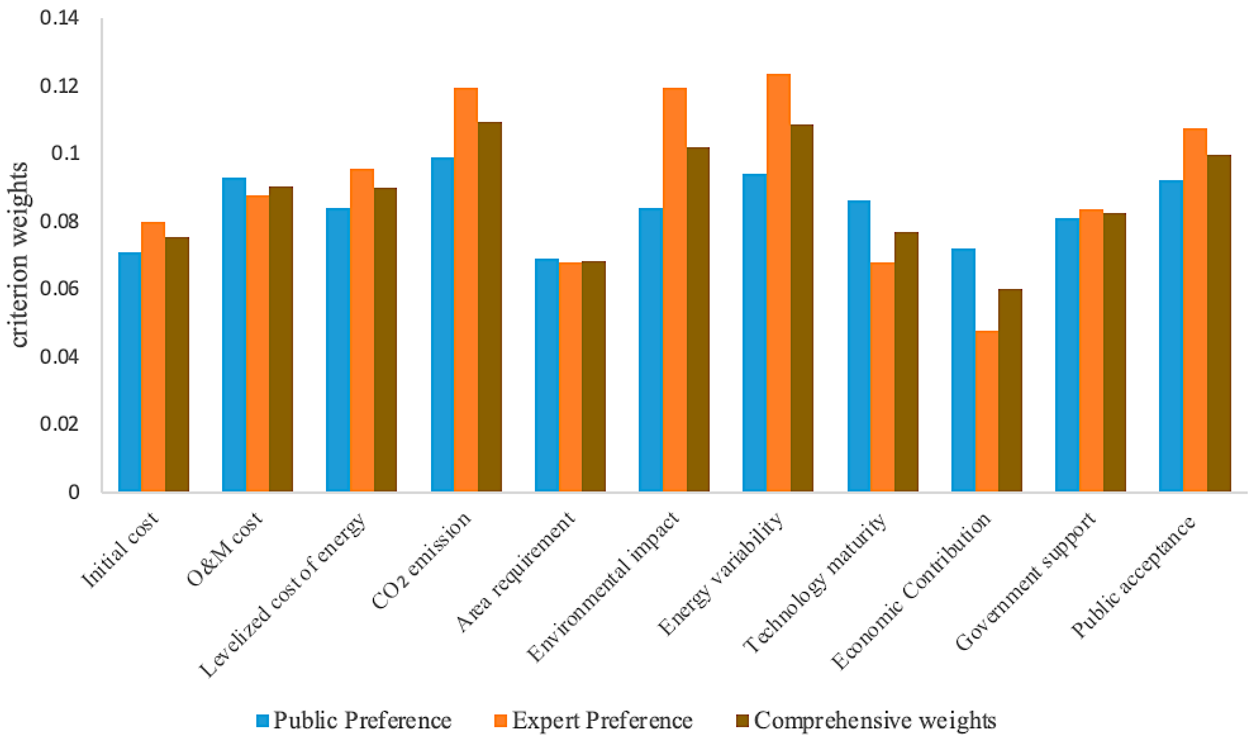
4.2.1. Criteria Weights

After the calculation of indicator weights based on indicators with credibility, the weighting results of each indicator were obtained. Table 11 shows the indicator weights based on public acceptance and the indicator weights based on expert ratings and the results. Among the results obtained from the citizens’ perspective, the indicator weight of carbon emission was the highest at 0.099, followed by energy volatility and social acceptability, while the indicator weight of floor area was the lowest at 0.069.
Meanwhile, Table 12. Displayed public preferences, expert preferences, and comprehensive indicator weights in the evaluation of indicator weights based on experts, the indicator of energy variability had the highest weight of 0.1235, followed by potential environmental impact and carbon emissions, and the indicator of industrial development contribution had the lowest weight of 0.08233.
Figure 8 illustrates the results of the evaluation of different indicators by the population and experts. The population had a more even distribution of the evaluation of the indicators compared to the experts, while the experts had a stronger bias towards the indicators. Carbon emissions and energy variability were the evaluation indicators of common concern for both residents and experts, which would be favorable aims to achieve a consensus between experts and citizens on the goals of energy promotion.

4.2.2. Alternative Scores

In this study, the alternatives were evaluated by considering the reliability of experts and residents, and the final scores of the alternatives were calculated using the BULI-EDAS method. The final ranking of the alternatives was A2 > A3 > A1 > A4 > A5 > A7 > A6 > A8. Alternative A2 was the best option, which achieved a better performance in terms of social acceptance, policy support, and energy stability, and was consistently recognized by experts and the public. Alternative A8, with a score of 0.3822, was the alternative with the worst overall performance, mostly due to its relatively high pollution, and because it holds no economic advantage from the perspective of long-term development. Figure 9 shows the positive and negative distances calculated by EDAS, and through Table 13, it can be found that alternatives A7 and A8 achieve better results in the positive distance, mainly because of the smaller occupation area and high energy stability level; however, alternatives A6, A7, and A8 performed poorly in the negative distance, resulting in a poor overall score.

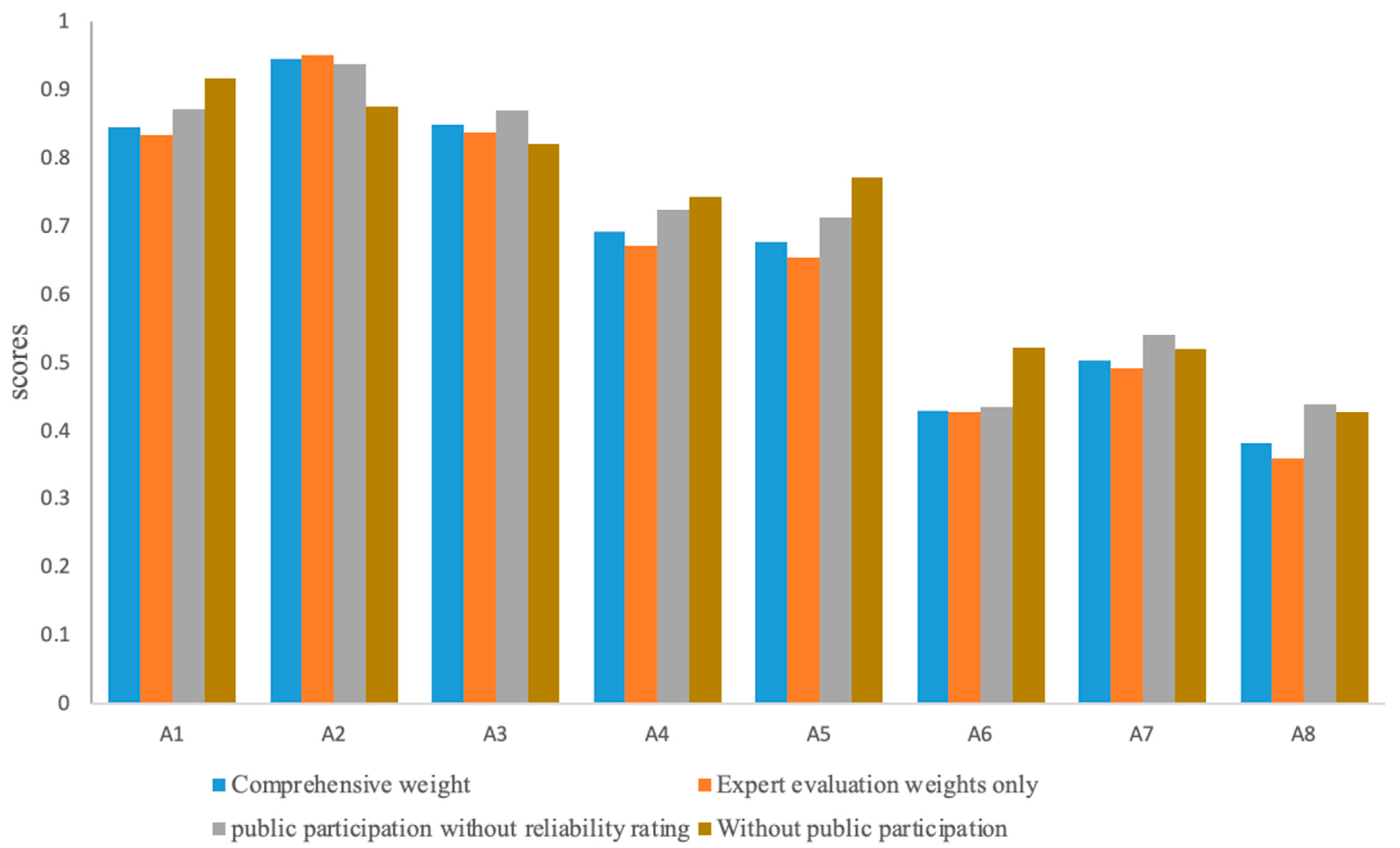
4.3. Comparative Analysis

In this section, a comparative analysis of the solutions under different weight allocation methods was conducted to verify the influence of different alternative ranking methods on the results. The alternative scores and ranking obtained by the different methods are shown in Figure 10 and Table 14, which shows that public participation and social acceptance of the solutions had a significant influence on the solutions. The results of this study were the same as the results of the criteria weighting evaluation by experts only, and the optimal alternative was A2. When public reliability is not considered, the optimal alternative was still A2, but the ranking of the options changed. Given the limited knowledge of citizens about some of the options, the reliability of decision makers’ opinions should be considered in the process. In addition, the results of the alternative ranking without considering public participation and the social acceptability of the alternatives were also compared; when the optimal alternative was A1 without considering public participation at all, the alternative ranking differed significantly from the other methods. Without considering social acceptance, the more economically efficient configurations had a significant advantage; however, the results may change after considering public opinion and social acceptance. The results of the analysis also indicate that both the social acceptability and the reliability of the public evaluation of the alternative are critical influencing factors that should be considered in the planning of HRESs.

4.4. Discussions

The results obtained in Section 4.2 and Section 4.3 show that the optimal alternative was A2 and the worst alternative was A8, and HRESs had significant advantages over the diesel generator alternative. The COE of A7 and A8 were 0.523 USD/kWh and 0.553 USD/kWh, respectively, ranking first and second in terms of cost and carbon emissions at 3,422,660 kg/year and 3,671,213 kg/year. Although the energy alternative of using a diesel generator required a smaller area and had greater energy stability and social acceptance, this option typically required higher energy costs and had intolerable carbon emissions, so using a diesel generator as the primary method of power generation in Bayin Wusu Village would not be the most economical or environmentally friendly choice. Alternative A6 is a 100% renewable energy solution. This solution has significant advantages in terms of reducing carbon emissions and environmental impacts, and it can also contribute to the local photovoltaic (PV) industry. However, solutions that heavily rely on renewable energy performed poorly on the energy stability index and may face the issue of insufficient load supply during extreme weather conditions. Meanwhile, the implementation of 100% renewable energy solutions require high initial investment cost, which led to the low feasibility of alternative A6. Alternatives A4 and A5 mainly rely on wind turbines for power generation. Due to the stable and abundant local wind energy resources and high policy support, alternatives mainly using wind energy performed well in all criteria, but the drawback was that the use of wind turbines for energy supply had a larger occupation area, which increased the negative distance of the option and reduced the feasibility. Alternatives A1–A3 were the complementary renewable energy alternative using different proportions; such schemes had better performance in economic and environmental indicators. Alternative A1 is a renewable energy system comprised entirely of solar panels and wind turbines and has a significant advantage in the COE index as it was the ideal renewable energy system option for this area. However, the energy stability and social acceptability scores were lower compared to other solutions because of the lack of diesel generators. Alternative A2 utilizes 1231 kW photovoltaic panels and 79 wind turbines, a 1700 kW diesel engine, and a 300 kW biogas generator, a combination of energy sources with improved energy stability while maintaining a high proportion of renewable energy sources and taking energy variability and social acceptability into consideration.
It is worth noting that social acceptability and public participation had a significant impact on system selection. The public generally tended to choose the more familiar and stable power system; therefore, the decision makers should popularize renewable energy knowledge before promoting HRESs so that the public can better understand the possible impacts of them. On the other hand, citizens should also learn more knowledge about clean energy, actively participate in the decisions of renewable energy processes, and accept and assist in the development of clean energy transitions.

5. Conclusions

HRESs have great potential for development by integrating various power generation technologies, reducing gas emissions, and improving energy stability while avoiding the shortcomings of single energy generation technologies. However, the promotion of clean energy projects needs to consider the residents’ willingness along with regional resources. Ensuring scientific and effective decision-making results under public participation poses a great challenge to decision makers. In this study, public evaluation was incorporated into the planning process and an HRES optimization model based on the reliability level of the decision maker was proposed. This makes the evaluation method of the target more comprehensive and convincing. To verify the feasibility of the model, the method was applied to the evaluation of HRES alternatives in Bayin Wusu Village in Mongolia, China. A total of 20 people and 7 experts participated in the decision-making process; 11 evaluation criteria and 8 feasible options were considered, and finally, the renewable energy option A2, which consists of a PV–turbine–biogas–diesel engine–energy storage system, was obtained as the optimal option. The selected HRES can provide sustainable and secure electricity for a total of 3140 residents in this area.
Based on the BULI-EDAS method, the optimal HRES energy solution was selected to significantly reduce CO2 emissions and environmental impacts while considering the acceptance of the residents, with a reduction in carbon emissions of 3625.9 t/year and a reduction in LCOE of 0.427 USD/kWh compared to the baseline solution. This study considered the planning and design of HRES energy schemes under the public participation mechanism, providing a new decision-making method and a reference for renewable energy planning. While promoting public understanding of HRES, it also contributes to the smooth implementation of the system; the resulting decision results integrate public will and expert knowledge to obtain a comprehensive optimal solution. However, the promotion of HRESs is still in the initial stage, and the process of public participation requires more time and higher costs to implement decisions. To ensure the effectiveness of the results, it is also necessary to ensure that the public has a sufficient understanding of the technical solutions and details, which puts higher requirements on system planners’ abilities.
Future research can consider the consensus and feedback mechanisms of experts’ and fairness, as well as the uncertainty of decision evaluation information, in order to improve scientific and rational decision making. Meanwhile, a topic worth studying in future research is a broader discussion of concepts, such as the paper [17], which may be encountered in situations where there is more participation from the public and opinions are more complex. Large group decision-making methods may be helpful in solving these problems. It should be noted that even when extended to a broader concept, the BULI-EDAS method proposed in this article can still have certain reference significance for the reliability issues evaluated by decision makers.

Author Contributions

Writing—original draft preparation, L.L.; methodology Y.Y.; conceptualization, X.C.; supervision, J.Y.; investigation, J.C. All authors have read and agreed to the published version of the manuscript.

Funding

This research was funded by National Natural Science Foundation of China grant number 72201097, National Natural Science Foundation of China grant number 62202160 and Natural Science Foundation of Hunan Province grant number 2021JJ40158.

Institutional Review Board Statement

Not applicable.

Informed Consent Statement

Not applicable.

Data Availability Statement

Not applicable.

Conflicts of Interest

The authors declare no conflict of interest.

Appendix A

Table A1. Assessment information given by DMs about the performances of alternative A2 according to various criteria.
Policy SupportEnergy VariabilityEnvironmental ImpactEconomic ContributionTechnology Maturity
D M 1 Δ s 3 ; 0.8 Δ s 3 ; 0.8 Δ s 2 ; 0.7 Δ s 2 ; 0.8 Δ s 2 ; 0.7
D M 2 Δ s 2 ; 1 Δ s 3 ; 0.9 Δ s 2 ; 1 Δ s 2 ; 0.5 Δ s 3 ; 1
D M 3 Δ s 3 ; 0.7 Δ s 3 ; 0.7 Δ s 2 ; 0.7 Δ s 3 ; 0.8 Δ s 2 ; 0.7
D M 4 Δ s 2 ; 0.5 Δ s 3 ; 0.6 Δ s 2 ; 0.6 Δ s 2 ; 0.6 Δ s 2 ; 0.7
D M 5 Δ s 3 ; 0.8 Δ s 3 ; 0.8 Δ s 2 ; 0.8 Δ s 1 ; 0.8 Δ s 1 ; 0.8
D M 6 Δ s 3 ; 0.8 Δ s 3 ; 0.7 Δ s 2 ; 0.7 Δ s 3 ; 0.7 Δ s 1 ; 0.7
D M 7 Δ s 2 ; 0.6 Δ s 2 ; 0.7 Δ s 2 ; 0.7 Δ s 2 ; 0.7 Δ s 2 ; 0.7
Table A2. Assessment information given by DMs about the performances of alternative A3 according to various criteria.
Policy SupportEnergy VariabilityEnvironmental ImpactEconomic ContributionTechnology Maturity
D M 1 Δ s 3 ; 0.6 Δ s 2 ; 0.6 Δ s 3 ; 0.8 Δ s 3 ; 0.8 Δ s 3 ; 0.7
D M 2 Δ s 4 ; 1 Δ s 3 ; 0.9 Δ s 3 ; 0.9 Δ s 2 ; 0.5 Δ s 3 ; 1
D M 3 Δ s 1 ; 0.5 Δ s 2 ; 0.5 Δ s 1 ; 0.5 Δ s 2 ; 0.5 Δ s 2 ; 0.6
D M 4 Δ s 3 ; 0.8 Δ s 3 ; 0.9 Δ s 3 ; 0.8 Δ s 3 ; 0.9 Δ s 4 ; 0.8
D M 5 Δ s 3 ; 0.8 Δ s 2 ; 0.7 Δ s 2 ; 0.7 Δ s 3 ; 0.7 Δ s 3 ; 0.7
D M 6 Δ s 3 ; 0.8 Δ s 2 ; 0.7 Δ s 2 ; 0.7 Δ s 2 ; 0.7 Δ s 2 ; 0.7
D M 7 Δ s 3 ; 0.7 Δ s 3 ; 0.8 Δ s 2 ; 0.8 Δ s 3 ; 0.7 Δ s 2 ; 0.7
Table A3. Assessment information given by DMs about the performances of alternative A4 according to various criteria.
Policy SupportEnergy VariabilityEnvironmental ImpactEconomic ContributionTechnology Maturity
D M 1 Δ s 3 ; 0.7 Δ s 2 ; 0.6 Δ s 3 ; 0.6 Δ s 3 ; 0.7 Δ s 4 ; 0.7
D M 2 Δ s 4 ; 1 Δ s 3 ; 0.8 Δ s 3 ; 0.9 Δ s 2 ; 0.5 Δ s 3 ; 0.8
D M 3 Δ s 2 ; 0.8 Δ s 3 ; 0.8 Δ s 3 ; 0.8 Δ s 3 ; 0.8 Δ s 3 ; 0.7
D M 4 Δ s 1 ; 0.6 Δ s 3 ; 0.5 Δ s 3 ; 0.4 Δ s 3 ; 0.6 Δ s 3 ; 0.5
D M 5 Δ s 2 ; 0.8 Δ s 3 ; 0.8 Δ s 3 ; 0.8 Δ s 3 ; 0.9 Δ s 3 ; 0.9
D M 6 Δ s 2 ; 0.7 Δ s 2 ; 0.7 Δ s 2 ; 0.7 Δ s 2 ; 0.7 Δ s 2 ; 0.7
D M 7 Δ s 2 ; 0.7 Δ s 2 ; 0.7 Δ s 2 ; 0.7 Δ s 2 ; 0.7 Δ s 2 ; 0.7
Table A4. Assessment information given by DMs about the performances of alternative A5 according to various criteria.
Policy SupportEnergy VariabilityEnvironmental ImpactEconomic ContributionTechnology Maturity
D M 1 Δ s 3 ; 0.6 Δ s 1 ; 0.4 Δ s 1 ; 0.7 Δ s 3 ; 0.8 Δ s 3 ; 0.9
D M 2 Δ s 4 ; 1 Δ s 3 ; 0.8 Δ s 3 ; 0.9 Δ s 2 ; 0.5 Δ s 3 ; 0.8
D M 3 Δ s 2 ; 0.8 Δ s 3 ; 0.8 Δ s 3 ; 0.8 Δ s 3 ; 0.8 Δ s 3 ; 0.8
D M 4 Δ s 2 ; 0.7 Δ s 1 ; 0.7 Δ s 3 ; 0.5 Δ s 1 ; 0.6 Δ s 1 ; 0.7
D M 5 Δ s 3 ; 0.8 Δ s 3 ; 0.7 Δ s 3 ; 0.8 Δ s 3 ; 0.9 Δ s 3 ; 0.9
D M 6 Δ s 2 ; 0.7 Δ s 1 ; 0.7 Δ s 2 ; 0.7 Δ s 2 ; 0.7 Δ s 2 ; 0.7
D M 7 Δ s 2 ; 0.7 Δ s 2 ; 0.7 Δ s 2 ; 0.7 Δ s 2 ; 0.7 Δ s 2 ; 0.7
Table A5. Assessment information given by DMs about the performances of alternative A6 according to various criteria.
Policy SupportEnergy VariabilityEnvironmental ImpactEconomic ContributionTechnology Maturity
D M 1 Δ s 2 ; 0.7 Δ s 1 ; 0.8 Δ s 2 ; 0.7 Δ s 3 ; 0.7 Δ s 4 ; 0.7
D M 2 Δ s 4 ; 1 Δ s 0 ; 1 Δ s 4 ; 1 Δ s 3 ; 0.6 Δ s 1 ; 1
D M 3 Δ s 2 ; 0.5 Δ s 1 ; 0.5 Δ s 3 ; 0.5 Δ s 1 ; 0.4 Δ s 1 ; 0.5
D M 4 Δ s 3 ; 0.4 Δ s 3 ; 0.5 Δ s 3 ; 0.4 Δ s 3 ; 0.5 Δ s 3 ; 0.5
D M 5 Δ s 3 ; 0.9 Δ s 1 ; 0.8 Δ s 3 ; 0.8 Δ s 3 ; 0.8 Δ s 2 ; 0.9
D M 6 Δ s 2 ; 0.7 Δ s 1 ; 0.7 Δ s 1 ; 0.7 Δ s 1 ; 0.7 Δ s 1 ; 0.7
D M 7 Δ s 2 ; 0.7 Δ s 2 ; 0.7 Δ s 2 ; 0.7 Δ s 2 ; 0.7 Δ s 2 ; 0.7
Table A6. Assessment information given by DMs about the performances of alternative A7 according to various criteria.
Policy SupportEnergy VariabilityEnvironmental ImpactEconomic ContributionTechnology Maturity
D M 1 Δ s 2 ; 0.7 Δ s 4 ; 0.7 Δ s 0 ; 0.7 Δ s 1 ; 0.7 Δ s 4 ; 0.8
D M 2 Δ s 1 ; 1 Δ s 4 ; 1 Δ s 1 ; 0.9 Δ s 2 ; 0.5 Δ s 4 ; 1
D M 3 Δ s 3 ; 0.8 Δ s 3 ; 0.8 Δ s 3 ; 0.8 Δ s 3 ; 0.8 Δ s 3 ; 0.8
D M 4 Δ s 3 ; 0.5 Δ s 3 ; 0.5 Δ s 3 ; 0.7 Δ s 1 ; 0.7 Δ s 1 ; 0.6
D M 5 Δ s 1 ; 0.8 Δ s 4 ; 0.8 Δ s 1 ; 0.8 Δ s 2 ; 0.7 Δ s 4 ; 0.8
D M 6 Δ s 1 ; 0.7 Δ s 1 ; 0.7 Δ s 1 ; 0.7 Δ s 1 ; 0.7 Δ s 1 ; 0.7
D M 7 Δ s 2 ; 0.7 Δ s 2 ; 0.7 Δ s 2 ; 0.7 Δ s 2 ; 0.7 Δ s 2 ; 0.7
Table A7. Assessment information given by DMs about the performances of alternative A8 according to various criteria.
Policy SupportEnergy VariabilityEnvironmental ImpactEconomic ContributionTechnology Maturity
D M 1 Δ s 1 ; 0.8 Δ s 4 ; 0.8 Δ s 3 ; 0.8 Δ s 1 ; 0.7 Δ s 4 ; 1
D M 2 Δ s 0 ; 1 Δ s 4 ; 1 Δ s 0 ; 1 Δ s 2 ; 0.5 Δ s 4 ; 1
D M 3 Δ s 2 ; 0.6 Δ s 2 ; 0.6 Δ s 2 ; 0.7 Δ s 4 ; 0.8 Δ s 3 ; 0.8
D M 4 Δ s 2 ; 0.7 Δ s 1 ; 0.7 Δ s 2 ; 0.6 Δ s 3 ; 0.6 Δ s 1 ; 0.6
D M 5 Δ s 1 ; 0.8 Δ s 4 ; 0.8 Δ s 2 ; 0.8 Δ s 2 ; 0.7 Δ s 4 ; 0.8
D M 6 Δ s 1 ; 0.7 Δ s 1 ; 0.7 Δ s 1 ; 0.7 Δ s 1 ; 0.8 Δ s 1 ; 0.7
D M 7 Δ s 2 ; 0.7 Δ s 2 ; 0.7 Δ s 2 ; 0.8 Δ s 2 ; 0.6 Δ s 2 ; 0.7

Appendix B

Questionnaire 1
Weighting of evaluation indicators for hybrid energy systems (Expert)
Thank you for taking the valuable time to fill out the questionnaire! This is an academic research questionnaire for evaluating the importance of evaluation indicators for hybrid renewable energy system solutions. Thank you for your support!
1.
What is your evaluation of the importance of initial investment indicators?
Very poor
poor
fair
good
very good
2.
What is your evaluation of the importance of operating cost indicators?
Very poor
poor
fair
good
very good
3.
What is your evaluation of the importance of standardized electricity indicators?
Very poor
poor
fair
good
very good
4.
What is your evaluation of the importance of carbon emission indicators?
Very poor
poor
fair
good
very good
5.
What is your evaluation of the importance of floor area indicators?
Very poor
poor
fair
good
very good
6.
What you evaluate the importance of potential environmental impact indicators?
Very poor
poor
fair
good
very good
7.
What is your evaluation of the importance of energy volatility indicators?
Very poor
poor
fair
good
very good
8.
What is your Evaluation of the importance of technical maturity indicators?
Very poor
poor
fair
good
very good
9.
What is your Evaluation of the Importance of Industrial Development Contribution Indicators?
Very poor
poor
fair
good
very good
10.
What is your evaluation of the importance of policy support indicators?
Very poor
poor
fair
good
very good
11.
What is your evaluation of the importance of social acceptance indicators?
Very poor
poor
fair
good
very good
Questionnaire 2
Weighting of evaluation indicators for hybrid energy systems (Public)
Thank you for taking the valuable time to fill out the questionnaire! This is an academic research questionnaire for evaluating the importance of evaluation indicators for hybrid renewable energy system solutions. Thank you for your support!
1.
What is your initial investment rating of the plan?
Very poor
poor
fair
good
very good
2.
What is the degree of certainty in your initial investment rating of the plan?
( ) Please enter a number between 0 and 1
3.
What is your operating cost rating of the plan?
Very poor
poor
fair
good
very good
4.
What is the degree of certainty in your operating cost rating of the plan?
( ) Please enter a number between 0 and 1
5.
What is your standardized electricity rating of the plan?
Very poor
poor
fair
good
very good
6.
What is the degree of certainty in your standardized electricity rating of the plan?
( ) Please enter a number between 0 and 1
7.
What is your carbon emission rating of the plan?
Very poor
poor
fair
good
very good
8.
What is the degree of certainty in your carbon emission rating of the plan?
( ) Please enter a number between 0 and 1
9.
What is your floor area rating of the plan?
Very poor
poor
fair
good
very good
10.
What is the degree of certainty in your floor area rating of the plan?
( ) Please enter a number between 0 and 1
11.
What is your environmental impact rating of the plan?
Very poor
poor
fair
good
very good
12.
What is the degree of certainty in your environmental impact rating of the plan?
( ) Please enter a number between 0 and 1
13.
What is your energy volatility rating of the plan?
Very poor
poor
fair
good
very good
14.
What is the degree of certainty in your energy volatility rating of the plan?
( ) Please enter a number between 0 and 1
15.
What is your technological maturity rating of the plan?
Very poor
poor
fair
good
very good
16.
What is the degree of certainty in your technological maturity rating of the plan?
( ) Please enter a number between 0 and 1
17.
What is your industrial Development Contribution rating of the plan?
Very poor
poor
fair
good
very good
18.
What is the degree of certainty in your industrial Development Contribution rating of the plan?
( ) Please enter a number between 0 and 1
19.
What is your policy support rating of the plan?
Very poor
poor
fair
good
very good
20.
What is the degree of certainty in your policy support rating of the plan?
( ) Please enter a number between 0 and 1
21.
What is your social acceptance rating of the plan?
Very poor
poor
fair
good
very good
22.
What is the degree of certainty in your social acceptance rating of the plan?
( ) Please enter a number between 0 and 1
Questionnaire 3
Evaluating the performance of indicators (Expert)
Thank you for taking the time to fill out the questionnaire! This is an academic research questionnaire mainly aimed at evaluating the performance of qualitative indicators for hybrid renewable energy system schemes. The problem is that there are currently 8 energy schemes, each of which is equipped with different proportions of renewable energy and corresponding components (as shown in the figure below). Please rate the overall qualitative indicators according to the configuration of the schemes. This questionnaire is a qualitative indicator evaluation for alternative (A1–A8), the remaining scheme will be collected in the same manner.
1.
What is your social acceptance rating of the plan?
Very poor
poor
fair
good
very good
2.
What is the degree of certainty in your social acceptance rating of the plan?
( ) Please enter a number between 0 and 1
3.
What is your policy support rating of the plan?
Very poor
poor
fair
good
very good
4.
What is the degree of certainty in your policy support rating of the plan?
( ) Please enter a number between 0 and 1
5.
What is your environmental impact rating of the plan?
Very poor
poor
fair
good
very good
6.
What is the degree of certainty in your environmental impact rating of the plan?
( ) Please enter a number between 0 and 1
7.
What is your economic development rating of the plan?
Very poor
poor
fair
good
very good
8.
What is the degree of certainty in your economic development rating of the plan?
( ) Please enter a number between 0 and 1
9.
What is your technological maturity rating of the plan?
Very poor
poor
fair
good
very good
10.
What is the degree of certainty in your technological maturity rating of the plan?
( ) Please enter a number between 0 and 1
Questionnaire 4
Public evaluation of social acceptance (Public)
Thank you for taking the valuable time to fill out the questionnaire! This is an academic research questionnaire for evaluating the performance of evaluation indicators for hybrid renewable energy system solutions. This questionnaire is a qualitative indicator evaluation for alternative (A1–A8), the remaining scheme will be collected in the same manner.
1.
What is your social acceptance rating of the plan?
Very poor
poor
fair
good
very good
2.
What is the degree of certainty in your social acceptance rating of the plan?
( ) Please enter a number between 0 and 1

Appendix C

Table A8. Details of Various Components.
ComponentItemValue
PVModel typeGeneric flat plate PV
Rated power1 kW/panel
Derating factor80%
Lifetime25 years
WTModel typeEocycle E010
Rated power10 kw
Cut-in velocity2.75 m/s
Cut-off velocity20 m/s
Rated velocity6.5 m/s
Hub height16 m
Lifetime20 years
BioGenFuel curve slope2.0 L/h/kW output
Intercept coefficient0.10 L/h/kW rated
Lifetime20,000 h
Carbon monoxide2 g/kg of fuel
Nitrogen oxides1.25 g/kg of fuel
Available biomass1.4287 tones/day
Gasification ratio0.7 kg
GeneratorFuel curve intercept25.9 L/h
Fuel curve slope0.236 L/h/kw
CO216.5 g/L fuel
Fuel price1USD/L
Lifetime20,000 h
BatteryBattery typeLead Acid
Minimal voltage12 V
Minimal capacity200 Ah
ConvertCapacity1 kW
Lifetime15 years
Inverter input efficiency95%
Relative capacity100%
Rectifier input efficiency95%
ElectrolyzerCapacity optimization{0,100,200,300}
Lifetime 15 years
Efficiency85%
Minimum load ratio0%

References

  1. Hu, J.; Harmsen, R.; Crijns-Graus, W.; Worrell, E. Barriers to investment in utility-scale variable renewable electricity (VRE) generation projects. Renew. Energy 2018, 121, 730–744. [Google Scholar] [CrossRef]
  2. Madurai Elavarasan, R.; Afridhis, S.; Vijayaraghavan, R.; Subramaniam, U.; Nurunnabi, M. SWOT analysis: A framework for comprehensive evaluation of drivers and barriers for renewable energy development in significant countries. Energy Rep. 2020, 6, 1838–1864. [Google Scholar] [CrossRef]
  3. Umamaheswaran, S.; Rajiv, S. Financing large scale wind and solar projects—A review of emerging experiences in the Indian context. Renew. Sustain. Energy Rev. 2015, 48, 166–177. [Google Scholar] [CrossRef]
  4. Bahramara, S.; Moghaddam, M.P.; Haghifam, M.R. Optimal planning of hybrid renewable energy systems using HOMER: A review. Renew. Sustain. Energy Rev. 2016, 62, 609–620. [Google Scholar] [CrossRef]
  5. Cuesta, M.A.; Castillo-Calzadilla, T.; Borges, C.E. A critical analysis on hybrid renewable energy modeling tools: An emerging opportunity to include social indicators to optimise systems in small communities. Renew. Sustain. Energy Rev. 2020, 122, 109691. [Google Scholar] [CrossRef]
  6. Ye, B.; Zhou, M.; Yan, D.; Li, Y. Multi-Objective Decision-Making for Hybrid Renewable Energy Systems for Cities: A Case Study of Xiongan New District in China. Energies 2020, 13, 6223. [Google Scholar] [CrossRef]
  7. Niu, D.; Zhen, H.; Yu, M.; Wang, K.; Sun, L.; Xu, X. Prioritization of renewable energy alternatives for China by using a hybrid FMCDM methodology with uncertain information. Sustainability 2020, 12, 4649. [Google Scholar] [CrossRef]
  8. Qiu, T.; Faraji, J. Techno-economic optimization of a grid-connected hybrid energy system considering electric and thermal load prediction. Energy Sci. Eng. 2021, 9, 1313–1336. [Google Scholar] [CrossRef]
  9. Ullah, Z.; Elkadeem, M.R.; Kotb, K.M.; Taha, I.B.M.; Wang, S. Multi-criteria decision-making model for optimal planning of on/off grid hybrid solar, wind, hydro, biomass clean electricity supply. Renew. Energy 2021, 179, 885–910. [Google Scholar] [CrossRef]
  10. Dawood, F.; Shafiullah, G.M.; Anda, M. Stand-Alone Microgrid with 100% Renewable Energy: A Case Study with Hybrid Solar PV-Battery-Hydrogen. Sustainability 2020, 12, 2047. [Google Scholar] [CrossRef]
  11. Jackson, T.; Oliver, M. Wind energy comes of age: Paul Gipe John Wiley, New York, 1995. Energy Policy 1996, 24, 491–492. [Google Scholar] [CrossRef]
  12. Diógenes, J.R.F.; Claro, J.; Rodrigues, J.C.; Loureiro, M.V. Barriers to onshore wind energy implementation: A systematic review. Energy Res. Soc. Sci. 2020, 60, 101337. [Google Scholar] [CrossRef]
  13. Estévez, R.A.; Espinoza, V.; Ponce Oliva, R.D.; Vásquez-Lavín, F.; Gelcich, S. Multi-Criteria Decision Analysis for Renewable Energies: Research Trends, Gaps and the Challenge of Improving Participation. Sustainability 2021, 13, 3515. [Google Scholar] [CrossRef]
  14. Zelt, O.; Krüger, C.; Blohm, M.; Bohm, S.; Far, S. Long-Term Electricity Scenarios for the MENA Region: Assessing the Preferences of Local Stakeholders Using Multi-Criteria Analyses. Energies 2019, 12, 3046. [Google Scholar] [CrossRef]
  15. Zhou, J.; Wu, Y.; Dong, H.; Tao, Y.; Xu, C. Proposal and comprehensive analysis of gas-wind-photovoltaic-hydrogen integrated energy system considering multi-participant interest preference. J. Clean. Prod. 2020, 265, 121679. [Google Scholar] [CrossRef]
  16. Dong, H.; Wu, Y.; Zhou, J.; Chen, W. Optimal selection for wind power coupled hydrogen energy storage from a risk perspective, considering the participation of multi-stakeholder. J. Clean. Prod. 2022, 356, 131853. [Google Scholar] [CrossRef]
  17. Zhang, Z.; Liao, H.; Tang, A. Renewable energy portfolio optimization with public participation under uncertainty: A hybrid multi-attribute multi-objective decision-making method. Appl. Energy 2022, 307, 118267. [Google Scholar] [CrossRef]
  18. Mesiar, R.; Borkotokey, S.; Jin, L.; Kalina, M. Aggregation Under Uncertainty. IEEE Trans. Fuzzy Syst. 2018, 26, 2475–2478. [Google Scholar] [CrossRef]
  19. Herrera, F.; Martinez, L. A 2-tuple fuzzy linguistic representation model for computing with words. IEEE Trans. Fuzzy Syst. 2000, 8, 746–752. [Google Scholar] [CrossRef]
  20. Chen, Z.-S.; Martínez, L.; Chang, J.-P.; Wang, X.-J.; Xionge, S.-H.; Chin, K.-S. Sustainable building material selection: A QFD- and ELECTRE III-embedded hybrid MCGDM approach with consensus building. Eng. Appl. Artif. Intell. 2019, 85, 783–807. [Google Scholar] [CrossRef]
  21. Li, J.; Liu, P.; Li, Z. Optimal design and techno-economic analysis of a hybrid renewable energy system for off-grid power supply and hydrogen production: A case study of West China. Chem. Eng. Res. Des. 2022, 177, 604–614. [Google Scholar] [CrossRef]
  22. Li, X.; Gao, J.; You, S.; Zheng, Y.; Zhang, Y.; Du, Q.; Xie, M.; Qin, Y. Optimal design and techno-economic analysis of renewable-based multi-carrier energy systems for industries: A case study of a food factory in China. Energy 2022, 244, 123174. [Google Scholar] [CrossRef]
  23. Mudasar, R.; Kim, M.-H. Experimental study of power generation utilizing human excreta. Energy Convers. Manag. 2017, 147, 86–99. [Google Scholar] [CrossRef]
  24. Yang, Y.; Bao, W.; Xie, G.H. Estimate of restaurant food waste and its biogas production potential in China. J. Clean. Prod. 2019, 211, 309–320. [Google Scholar] [CrossRef]
  25. Barber, S.; Boller, S.; Nordborg, H. Feasibility study for 100% renewable energy microgrids in Switzerland. Wind Energ. Sci. Discuss. 2019, 16. [Google Scholar] [CrossRef]
  26. Chauhan, A.; Saini, R.P. Techno-economic feasibility study on Integrated Renewable Energy System for an isolated community of India. Renew. Sustain. Energy Rev. 2016, 59, 388–405. [Google Scholar] [CrossRef]
  27. Baruah, A.; Basu, M.; Amuley, D. Modeling of an autonomous hybrid renewable energy system for electrification of a township: A case study for Sikkim, India. Renew. Sustain. Energy Rev. 2021, 135, 110158. [Google Scholar] [CrossRef]
  28. Rad, M.A.V.; Ghasempour, R.; Rahdan, P.; Mousavi, S.; Arastounia, M. Techno-economic analysis of a hybrid power system based on the cost-effective hydrogen production method for rural electrification, a case study in Iran. Energy 2020, 190, 116421. [Google Scholar] [CrossRef]
  29. Akhtari, M.R.; Baneshi, M. Techno-economic assessment and optimization of a hybrid renewable co-supply of electricity, heat and hydrogen system to enhance performance by recovering excess electricity for a large energy consumer. Energy Convers. Manag. 2019, 188, 131–141. [Google Scholar] [CrossRef]
  30. Ramezanzade, M.; Saebi, J.; Karimi, H.; Mostafaeipour, A. A new hybrid decision-making framework to rank power supply systems for government organizations: A real case study. Sustain. Energy Technol. Assess. 2020, 41, 100779. [Google Scholar] [CrossRef]
  31. Jing, R.; Wang, M.; Brandon, N.; Zhao, Y. Multi-criteria evaluation of solid oxide fuel cell based combined cooling heating and power (SOFC-CCHP) applications for public buildings in China. Energy 2017, 141, 273–289. [Google Scholar] [CrossRef]
  32. Li, T.; Li, A.; Guo, X. The sustainable development-oriented development and utilization of renewable energy industry—A comprehensive analysis of MCDM methods. Energy 2020, 212, 118694. [Google Scholar] [CrossRef]
  33. Wu, Y.; Zhang, T.; Gao, R.; Wu, C. Portfolio planning of renewable energy with energy storage technologies for different applications from electricity grid. Appl. Energy 2021, 287, 116562. [Google Scholar] [CrossRef]
  34. Saraswat, S.K.; Digalwar, A.; Yadav, S.S. Development of assessment model for selection of sustainable energy source in India: Hybrid fuzzy MCDM approach. In International Conference on Intelligent and Fuzzy Systems; Springer: Berlin/Heidelberg, Germany, 2020; pp. 649–657. [Google Scholar]
  35. Zhang, L.; Zhou, P.; Newton, S.; Fang, J.; Zhou, D.; Zhang, L. Evaluating clean energy alternatives for Jiangsu, China: An improved multi-criteria decision making method. Energy 2015, 90, 953–964. [Google Scholar] [CrossRef]
  36. Zavadskas, E.K. Multi-Criteria Inventory Classification Using a New Method of Evaluation Based on Distance from Average Solution (EDAS). Informatica 2015, 26, 435–451. [Google Scholar] [CrossRef]
Figure 1. Hourly electrical energy demand of the study area.
Sustainability 15 08454 g001
Figure 2. Hourly electrical energy demand of a rural household.
Sustainability 15 08454 g002
Figure 3. Monthly average temperature.
Sustainability 15 08454 g003
Figure 4. Monthly average wind speed.
Sustainability 15 08454 g004
Figure 5. Monthly average solar radiation.
Sustainability 15 08454 g005
Figure 6. The framework of the optimization method.
Sustainability 15 08454 g006
Figure 7. Adopted indices for performance assessment of different alternatives.
Sustainability 15 08454 g007
Figure 8. Comparison of criterion weight using the MCDM method.
Sustainability 15 08454 g008
Figure 9. Alternatives’ performances based on EDAS algorithm.
Sustainability 15 08454 g009
Figure 10. Alternatives’ scores using different settings of criteria weights.
Sustainability 15 08454 g010
Table 1. Load demand estimation of a rural household.
ItemConsumption (W/Unit)Qty
(Unit)
SummerWinter
Daily
Operating Hours (h)
kWh/dayDaily
Operating Hours (h)
kWh/day
Lights (CFLs)24580.9680.96
TV60140.2440.24
Cell phone charger10320.0610.03
Refrigerator1501243.6243.6
Air conditioner800223.200
Fan50250.500
Water pumps175110.17520.35
Iron100010022
Total load of household (kWh/day)
Total public demand (kWh/day)
8.97 8.42
10,970.3 10,297.66
Table 2. Load demand estimation for different energy consumption sectors.
Public Demand
Energy Consumption SectorItemConsumption (W/Unit)Qty
(Unit)
Daily
Operating Hours Summer/Winter
Energy Demand (kWh)
Summer/Winter
SchoolLights (CFL)24605/514.4/14.4
Fan50605/015/0
Computer20308/860/60
HospitalLights (CFL)243010/107.2/7.2
Fan50305/07.5/0
Computer250188/836/36
Refrigerator150524/2418/18
Commercial/industrial
Flourmill 375048/8120/120
Mini dairy plant 500048/8160/160
Shop 2010/899.2/99.2
Agricultural use
Agricultural:Irrigation pump500086/6240/240
Crop threshing machine140083/333.6/33.6
Lights (CFL)24106/61.44/1.44
Total Energy demand (kWh/day) 812.34/789.84
Table 3. Biomass resource estimation.
Type of Raw
Material
Number of HeadsRaw Material Available per Head per Day (kg)Collection Coefficient Daily Total Biomass Production (ton)
Human Excreta31400.350.70.7693
Kitchen Waste31400.30.70.6594
Total Biomass Production 1.4287
Table 4. Area required for various components.
ComponentArea
Required
Ref.
PV System180 W/m2[24]
Wind Turbine0.92 m2/turbine[25]
Biogas System13.44 m2/kW[25]
Battery0.095 m2/unit[26]
Converter464 m2/unit[26]
Table 5. Financial details of various components.
ComponentCapital (USD)Replacement (USD)Maintenance
(USD)
LifetimeRef.
Diesel generator300/kw300/kw0.01/h90,000 h[27]
Wind Turbine20,000/turbine18,000/turbine600/year20 years[10]
PV System900/kw850/kw10/year20 years[21]
Hydrogen Tank600/kg600/kg10/year20 years[28]
Electrolyzer1500/kw1500/kw0.05/h10 years[28]
Biogas System1500/kw1500/kw0.01/h200 h[10]
Boiler54/kw54/kw0/kw20 years[29]
Converter300/kw300/kw0/kw15 years[29]
Battery500/kw500/kw0/hour15 years[21]
Table 6. Details of parameters setting imposed in this study.
System Parameter Setting
Interest Rate8%
Inflation Rate2%
Carbon Price3 USD/t
Project Life25 years
Annual Capacity Shortage0%
Table 7. List of evaluating indicators for alternatives.
DimensionsIndicatorAttribute TypeRef.
EconomyInitial cost (Q1)Quantitative[30]
O&M cost (Q2)Quantitative[27]
Levelized cost of energy (Q3)Quantitative[31]
EnvironmentCO2 emissions (Q4)Quantitative[30]
Area requirement (Q5)Quantitative[27]
Environmental impact (Q6)Qualitative[32]
TechnologyEnergy variability (Q7)Qualitative[32]
Technology maturity (Q8)Qualitative[33]
SocietyEconomic contribution (Q9)Qualitative[16]
Policy support (Q10)Qualitative[7,34]
Public acceptance (Q11)Qualitative[35]
Table 8. Summary of the design optimization results of different HRES configurations.
AlternativePV (kW)EO10 (10 kW)Gen (kW)Bio (kW)1 kWh LAElectrolyzer (kW)HTank (kg)Converter (kW)
A11453.8496 30018,4411001501356
A21005.1480170030016,3712001501327
A31231.79791700 17,1882001501633
A4 108170030014,9692002001268
A5 1361700 15,7961002001496
A613,915.17 20021,733200501658
A7 1700100629100300253
A8 1700 114510050200
Table 9. Summary of the assessment criteria results of different configurations.
AlternativeCOE (USD/kWh)Initial Capital (USD)O&M (USD/yr)CO2 (kg/yr)Area (m2)
A10.1235,072,64287,581.09454.14984,171.53
A20.1265,244,21086,301.1345,305.5675,108.58
A30.1295,257,08579,652.2866,507.7675,144.60
A40.1334,858,919106,969.8139,374.380,255.15
A50.1395,078,761104,909.4161,908.888,975.04
A60.31714,401,370161,052.141.65579,879.87
A70.5231,387,371441,537.83,422,660378.26
A80.5531,147,346460,347.83,671,213134.28
Table 10. Assessment information given by DMs about the performances of alternative A1 according to various criteria.
Government SupportEnergy
Variability
Environmental ImpactEconomic
Contribution
Technology Maturity
D M 1 Δ s 3 ; 0.7 Δ s 2 ; 0.6 Δ s 3 ; 0.8 Δ s 3 ; 0.7 Δ s 4 ; 0.8
D M 2 Δ s 3 ; 1 Δ s 1 ; 1 Δ s 4 ; 1 Δ s 3 ; 0.5 Δ s 3 ; 1
D M 3 Δ s 2 ; 0.6 Δ s 2 ; 0.6 Δ s 2 ; 0.6 Δ s 3 ; 0.7 Δ s 1 ; 0.6
D M 4 Δ s 3 ; 0.5 Δ s 2 ; 0.5 Δ s 3 ; 0.5 Δ s 2 ; 0.6 Δ s 2 ; 0.5
D M 5 Δ s 2 ; 0.9 Δ s 2 ; 0.8 Δ s 2 ; 0.8 Δ s 3 ; 0.7 Δ s 2 ; 0.8
D M 6 Δ s 3 ; 0.6 Δ s 2 ; 0.8 Δ s 1 ; 0.7 Δ s 2 ; 0.7 Δ s 2 ; 0.7
D M 7 Δ s 3 ; 0.7 Δ s 3 ; 0.8 Δ s 2 ; 0.8 Δ s 3 ; 0.7 Δ s 2 ; 0.7
Table 11. Aggregated group preference matrix.
Government SupportEnergy VariabilityEnvironmental ImpactEconomic ContributionTechnology Maturity
A1 Δ s 4.143 ; 0.714 Δ s 2.741 ; 0.729 Δ s 3.429 ; 0.743 Δ s 3.429 ; 0.657 Δ s 3.143 ; 0.729
A2 Δ s 3.857 ; 0.743 Δ s 4 ; 0.743 Δ s 3.571 ; 0.743 Δ s 3.571 ; 0.7 Δ s 3.429 ; 0.757
A3 Δ s 3.667 ; 0.733 Δ s 3.333 ; 0.717 Δ s 3.333 ; 0.733 Δ s 3.5 ; 0.683 Δ s 3.883 ; 0.75
A4 Δ s 3.286 ; 0.757 Δ s 3.571 ; 0.7 Δ s 3.741 ; 0.4 Δ s 3.571 ; 0.7 Δ s 3.857 ; 0.714
A5 Δ s 3.571 ; 0.7 Δ s 3 ; 0.686 Δ s 3.429 ; 0.729 Δ s 3.286 ; 0.714 Δ s 3.429 ; 0.786
A6 Δ s 3.571 ; 0.7 Δ s 2.286 ; 0.714 Δ s 3.571 ; 0.686 Δ s 3.143 ; 0.629 Δ s 3 ; 0.714
A7 Δ s 2.857 ; 0.743 Δ s 4 ; 0.743 Δ s 2.571 ; 0.757 Δ s 2.714 ; 0.686 Δ s 3.714 ; 0.771
A8 Δ s 2.143 ; 0.757 Δ s 3.571 ; 0.757 Δ s 2.741 ; 0.757 Δ s 3.143 ; 0.686 Δ s 3.714 ; 0.8
Table 12. Estimated criterion weights.
CriterionPublic PreferenceExpert PreferenceComprehensive Weights
Initial cost (Q1)0.0710.079680.07534
O&M cost (Q2)0.0930.087640.09032
Levelized cost of energy (Q3)0.0840.09560.0898
CO2 emissions (Q4)0.0990.11950.10925
Area requirement (Q5)0.0690.067720.06836
Environmental impact (Q6)0.0840.11950.10175
Energy variability (Q7)0.0940.12350.10875
Technology maturity0.0860.067720.07686
Economic contribution (Q9)0.0720.04780.0599
Policy support (Q10)0.0810.083660.08233
Public acceptance (Q11)0.0920.10750.09975
Table 13. The normalized PDA and NDA scores, EDAS score, and ranking of all feasible alternatives.
AlternativeWeighted Sum of PDAWeighted Sum of NDAWeighted Normalized
PDA
Weighted Normalized
NDA
EDAS SCORERank
A10.16570.05950.85390.83540.84473
A20.19400.039710.89010.94501
A30.15120.029340.77960.91900.84932
A40.10220.051760.52680.85690.69184
A50.11390.085330.58690.76420.67555
A60.09050.220240.46670.39140.42917
A70.14790.274770.76260.24070.50176
A80.14830.361920.764400.38228
Table 14. Comparison of alternatives, ranked using different weighting methods.
MethodRanking of Alternatives
Comprehensive weightsA2 > A3 > A1 > A4 > A5 > A7 > A6 > A8
Expert evaluation weights onlyA2 > A3 > A1 > A4 > A5 > A7 > A6 > A8
Public participation without reliability ratingA2 > A1 > A3 > A4 > A5 > A7 > A8 > A6
Without public participationA1 > A2 > A3 > A5 > A4 > A6 > A7 > A8
Disclaimer/Publisher’s Note: The statements, opinions and data contained in all publications are solely those of the individual author(s) and contributor(s) and not of MDPI and/or the editor(s). MDPI and/or the editor(s) disclaim responsibility for any injury to people or property resulting from any ideas, methods, instructions or products referred to in the content.

