Mining Method Optimization of Difficult-to-Mine Complicated Orebody Using Pythagorean Fuzzy Sets and TOPSIS Method

Abstract

In Suichang gold mine, the altered rock type gold deposits were cut by faults and joint fissures, leading to complex resource endowment characteristics, large changes in occurrence, a serious complex of ore vein branches and great difficulty in mining. In order to select a suitable mining method for such a difficult and complicated orebody, a multi-factor and multi-index comprehensive evaluation system involving benefits, costs, safety and other aspects was constructed by using the Pythagorean fuzzy sets and TOPSIS method. Taking Suichang gold mine as an example, the weighted aggregation evaluation matrix was constructed, the closeness index of the four mining schemes were 0.8436, 0.3370, 0.4296 and 0.4334, and the mechanized upward horizontal layering method was determined as the optimal scheme. This method overcame the fuzzy comparison of economic and technical indicators directly, but converted them into corresponding fuzzy numbers to obtain accurate closeness index for optimization. The application of this method not only ensured a safe, efficient and environment-friendly mining effect, but also provided a reference for the optimization of the mining scheme of the severely branched composite orebody.

1. Introduction

In the design process of new mines and reconstruction and upgrading of mines, the design of mining methods is an important part and is the core of the whole design work, which directly determines the subsequent technical personnel allocation, production organization management and industrial supporting facilities [1,2,3]. Choosing the most appropriate mining method to mine the deposit is very important to the safety, economy and environmental protection of mining operations and affects the benefits and long-term development of mining companies [4].

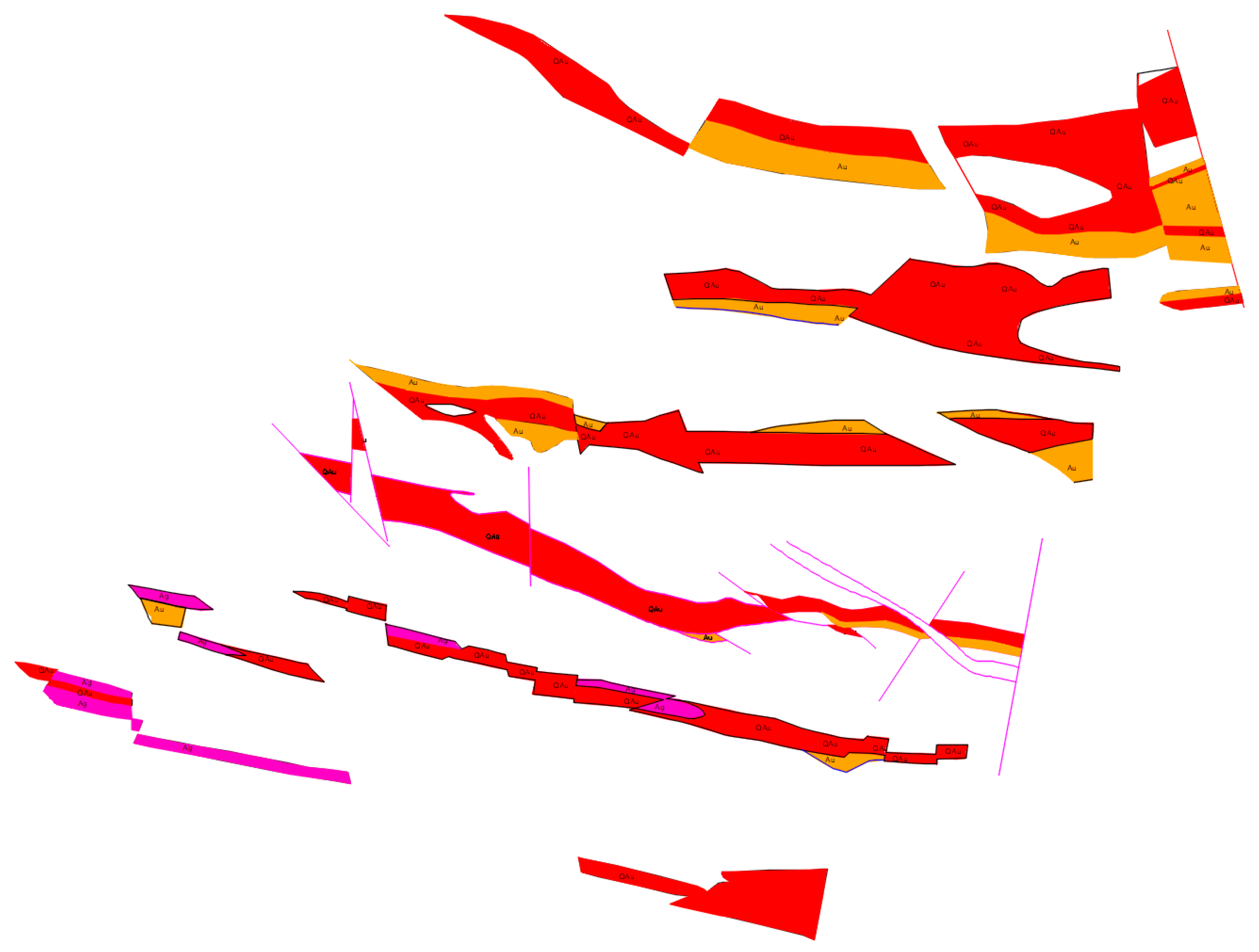
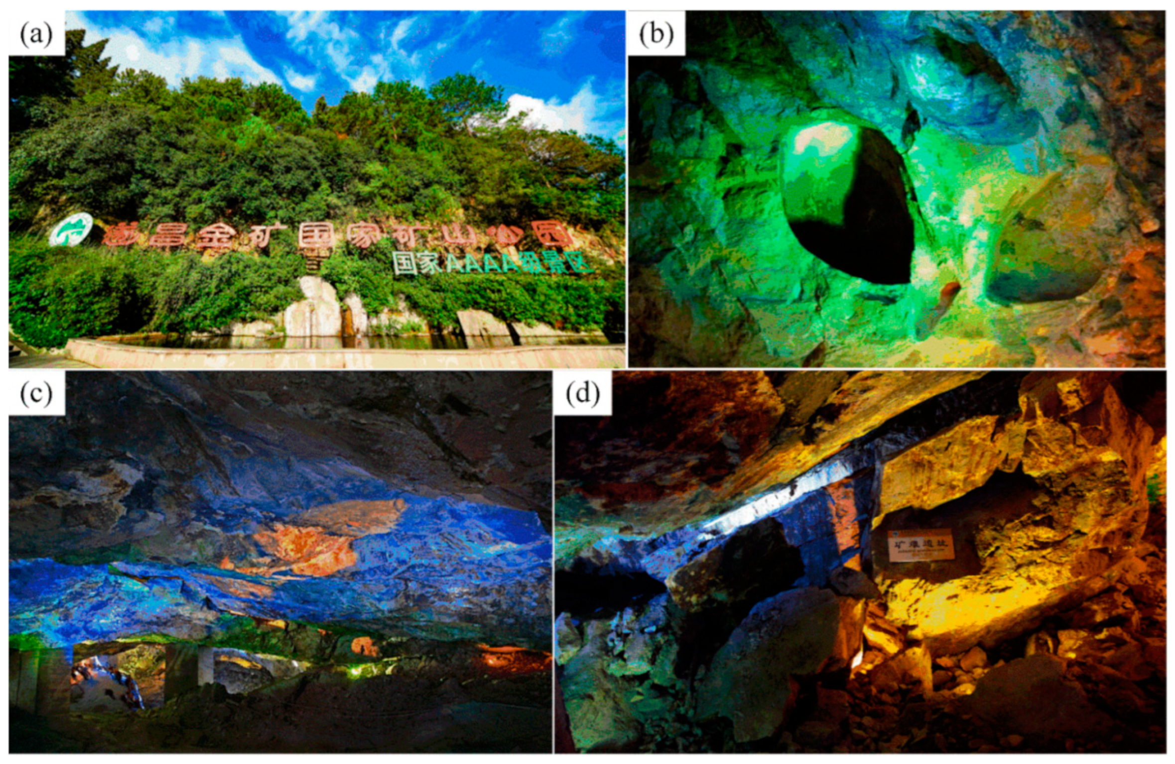
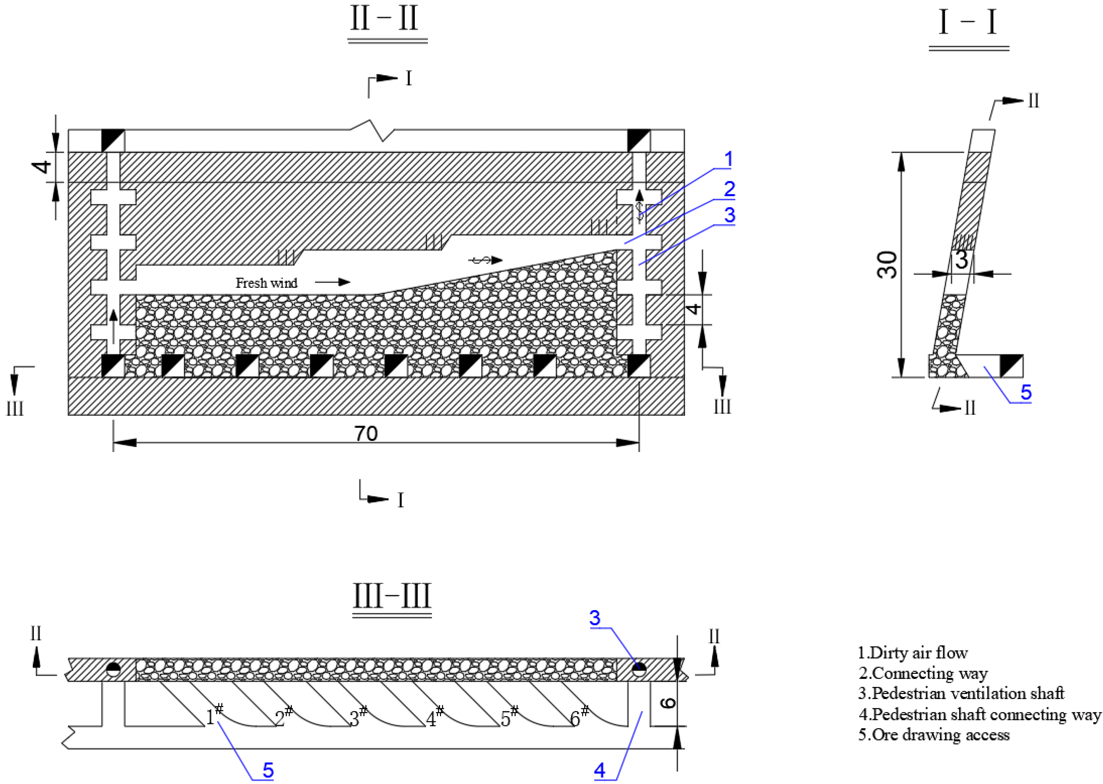
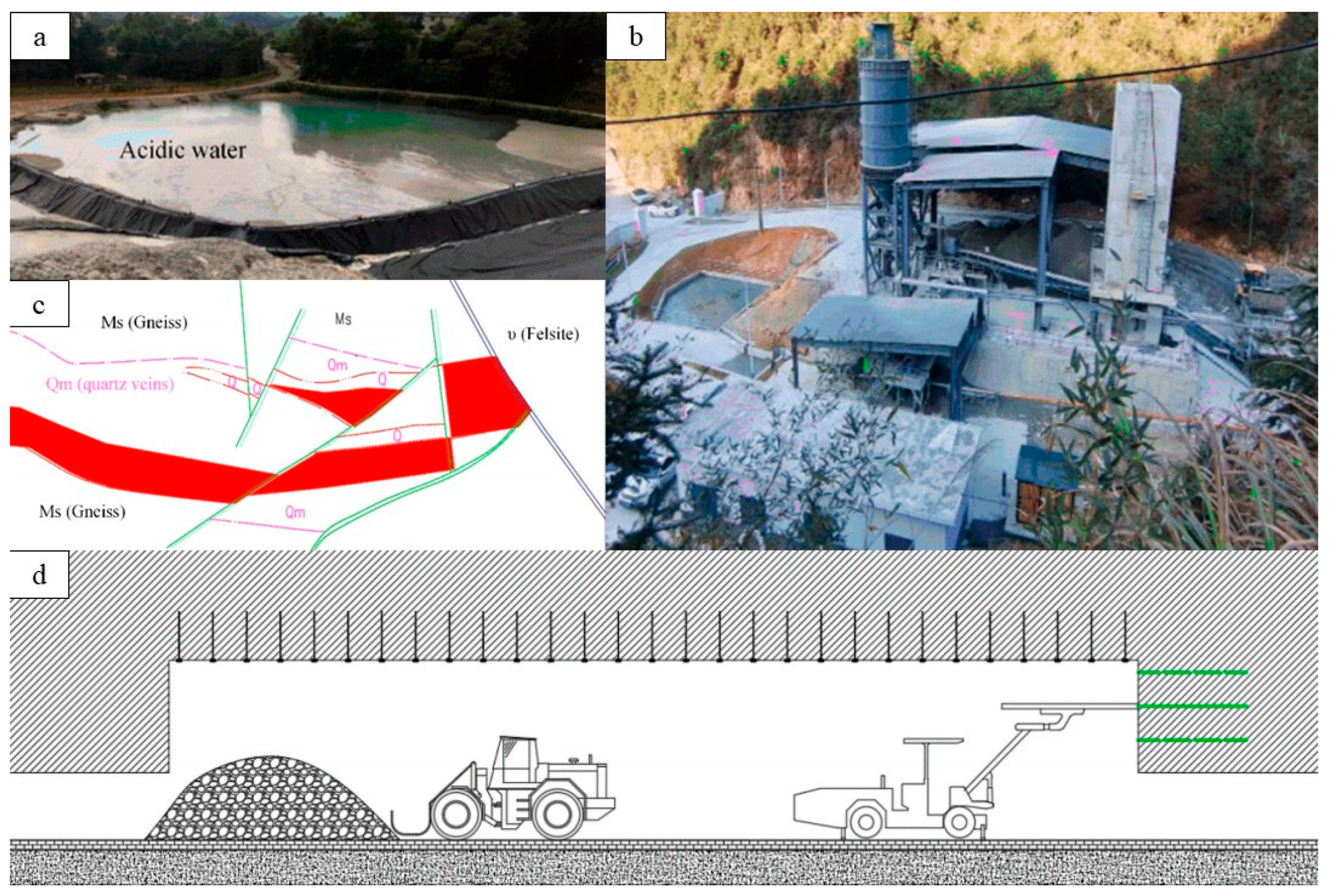
For a continuous orebody with regular shape, the most appropriate mining method can be selected by comparing the advantages and disadvantages and the economic and technical indicators. However, taking the difficult-to-mine complicated orebody (DCO) (see Figure 1) as example, it was greatly affected by faults and joint fissures, leading to obvious branching and compounding phenomenon. Since it is difficult to determine the optimal plan through traditional methods for DCO, more reliance is placed on the experience of design decision-makers and limited data, through the comprehensive comparison of various indicators. This is typical of Multiple Attribute Decision Making (MADM).

Multiple Attribute Decision Making refers to the decision making problem of selecting the best alternative or ranking under a condition of considering multiple indicators [5]. In order to solve such problems, researchers have developed a variety of multi criteria decision-making methods; typical representative methods include the Analytic Hierarchy Process [6], Entropy method [7], CRITIC method [8], TOPSIS method [9], GST (Grey Target Decision) method [10], DEA method [11], VIKOR method [12], Fuzzy comprehensive evaluation method [13], etc.

However, with increase in the complexity and scientific requirements of evaluation, a single decision-making method cannot guarantee optimal or accurate results [14,15]. Under this background, researchers have explored and developed mixed decision-making methods, for example, mixtures of Analytic Hierarchy Process and fuzzy, Entropy weight method and TOPSIS, Analytic Hierarchy Process, fuzzy set and VIKOR, fuzzy set and TOPSIS, etc.

In the field of mining engineering, many experts rely on these decision-making methods to optimize mining methods, for example, Karimnia [16] proposed the fuzzy analytical hierarchy process method, the most suitable method selected for Iran’s Qapliq salt mine. Yavuz [17] used the AHP method and fuzzy multiple attribute decision-making method, respectively, in a lignite mine located in Istanbul, carried out sensitivity analysis of the two methods and concluded that the Room and pillar method with filling is the most appropriate method. Qinqiang Guo [18] used the mixed method of AHP to determine the index weight and TOPSIS to rank, selecting the most suitable mining method from the Soft Broken Complex Orebody, and achieved very good results, Iphar [19] is committed to developing a mobile application, integrating several decision-making methods, and the optimal mining method can be obtained by inputting the original parameters for reference by engineering researchers.

However, in view of the complexity of mining method selection, simple expert scoring cannot fully reflect the fuzzy information, and the cognitive differences between different experts are easy to cause distortion of results. In terms of sorting, different ranging methods may have different results. In this case, the development of fuzzy set theory provides a good idea for solving such problems [20]. Bajić [21] transformed the indicators into triangular fuzzy numbers, constructed a fuzzy decision matrix and a fuzzy performance matrix, used to select the optimal alternative, and verified this through sensitivity analysis. Memori [22] uses the TOPSIS method based on intuitionistic fuzzy sets, providing an accurate sustainable ranking of suppliers and a relevant solution for sustainable sourcing decisions that is validated through a real-world case study. Narayanamoorthy [23] selected the best scheme for the selection of industrial robots by using a combination of Interval-valued intuitionistic hesitant fuzzy entropy and VIKOR.

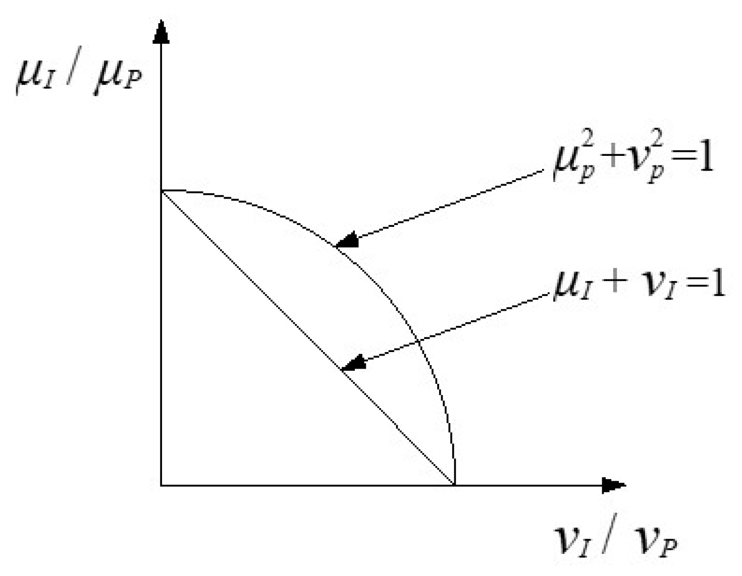
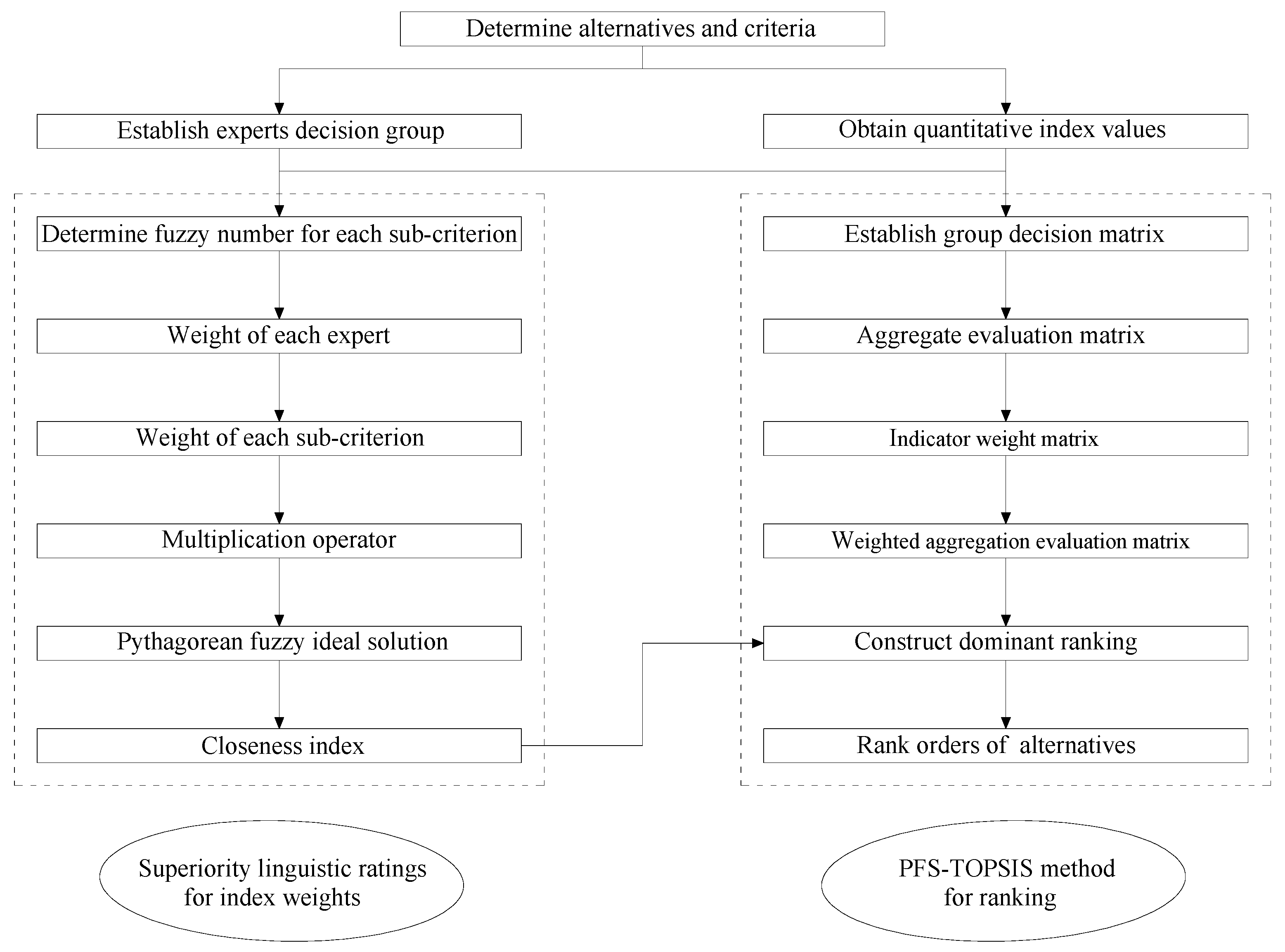
Pythagorean fuzzy sets (PFS) generalized by Yager [24] is a new method to deal with fuzzy problems. Its main contribution is to go beyond the limit that the sum of membership and no membership of fuzzy sets is less than 1 (see Figure 2). Compared with other fuzzy sets such as intuitionistic fuzzy sets, it can more fully and accurately represent uncertain information [25]. In view of this, this paper introduces a TOPSIS method based on PFS [26]. 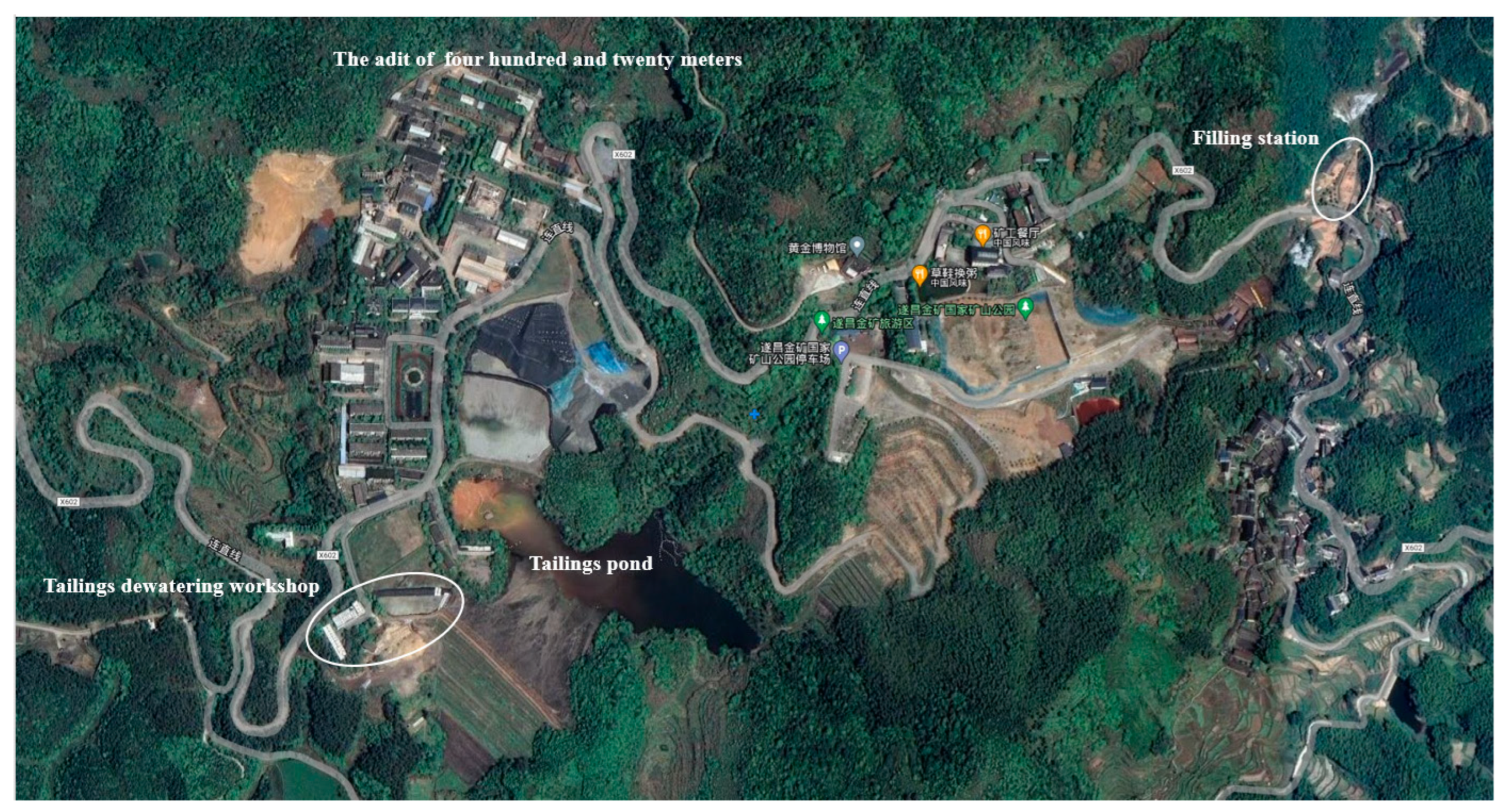The framework of this PFS–TOPSIS method is illustrated (see Figure 3), which is used for mining method decision-making for the Suichang Gold Mine in Zhejiang Province, China, and has achieved good results in actual production.

2. Methods Introduction

2.1. Introduction of PFS Method

Definition 1.

Let X be a universe of discourse [27,28]. The PFS ξ on X is given by Equation (1).

$$\xi =\left\{\left[x,{\mu }_{\xi }\left(x\right),{\nu }_{\xi }\left(x\right)|xϵX\right]\right\}$$

(1)

where the functions μ_ξ(x):X → [0, 1] and ν_ξ(x): X → [0, 1] define the degree of membership and the degree of non-membership of the element x∈X to the set ξ, respectively, with the condition that 0 ≤ (μ_ξ(x))² + (ν_ξ(x))² ≤ 1,∀x∈X. π_ξ(x) =$\sqrt{1-{\left({\mu }_{\xi }\left(x\right)\right)}^2-{\left({\nu }_{\xi }\left(x\right)\right)}^2}$is called the degree of indeterminacy of element x∈X. For convenience, they are called (μ_ξ(x), ν_ξ(x)) and a Pythagorean fuzzy number (PFN) denoted by ξ = (μ_ξ,ν_ξ,) [29].

Definition 2.

For the collection ξ_i = (μ_ξ,ν_ξ,) (i = 1,2,……n) of the of PFNs with the weight vector w = (w₁ w₂……w_n) of ξ_i(i = 1,2,……n) such that${\displaystyle \sum _{i=1}^n} w_i=1$, the Pythagorean fuzzy weighted averaging (PFWA) operator and the Pythagorean fuzzy weighted geometric (PFWG) operator can be defined as in Equations (2) and (3), respectively [30].

$$\begin{array}{ll}PFW{A}_w\left({\xi }_1,{\xi }_2,\cdots ,{\xi }_n\right)& =w_1{\xi }_1\oplus w_2{\xi }_2\oplus \cdots \oplus w_n{\xi }_n\hfill \\ & =\left(\sqrt{1-{\displaystyle \prod _{i=1}^n{\left(1-{\left({\mu }_{{\xi }_i}\right)}^2\right)}^{w_i}}},{\displaystyle \prod _{i=1}^n{\left({\nu }_{{\xi }_i}\right)}^{w_i}}\right),\hfill \end{array}$$

(2)

$$\begin{array}{ll}PFW{G}_w\left({\xi }_1,{\xi }_2,\cdots ,{\xi }_n\right)& =w_1{\xi }_1\otimes w_2{\xi }_2\otimes \cdots \otimes w_n{\xi }_n\hfill \\ & =\left({\displaystyle \prod _{i=1}^n{\left({\mu }_{{\xi }_i}\right)}^{w_i}},\sqrt{1-{\displaystyle \prod _{i=1}^n{\left(1-{\left({\upsilon }_{{\xi }_i}\right)}^2\right)}^{w_i}}}\right).\hfill \end{array}$$

(3)

Definition 3.

Let A and B be PFSs of X = {x₁, x₂, … x_n} [27]. Then, the sum of A and B is defined as Equation (4).

$$\begin{array}{cc}A\oplus B=& \{\langle x,\sqrt{{\left({\mu }_A\left(x\right)\right)}^2+{\left({\mu }_B\left(x\right)\right)}^2-{\left({\mu }_A\left(x\right)\right)}^2{\left({\mu }_B\left(x\right)\right)}^2},\hfill \\ & {\nu }_A\left(x\right){\nu }_B\left(x\right)\rangle \mid x\in X\},\hfill \end{array}$$

(4)

The product of A and B is defined as Equation (5).

$$\begin{array}{cc}A\otimes B=& \{ \langle x,{\mu }_A\left(x\right){\mu }_B\left(x\right),\hfill \\ & \sqrt{{\left({\nu }_A\left(x\right)\right)}^2+{\left({\nu }_B\left(x\right)\right)}^2-{\left({\nu }_A\left(x\right)\right)}^2{\left({\nu }_B\left(x\right)\right)}^2}\rangle \mid x\in X\}.\hfill \end{array}$$

(5)

2.2. Introduction of TOPSIS Method

The TOPSIS method was developed by Hwang [31], first put forward in 1981, and is a method of ranking according to the closeness of a limited number of evaluation objects to the ideal target. After years of development, dozens of derivative methods have been created by combining various mathematical theories, and have been widely used in various fields such as economic, management, engineering, medicine, etc. Its core ideas and steps are as follows [32]:

(1)

Quantification of evaluation indicators, converting natural language into numbers, and ensuring a certain distinction between good and bad, D is the evaluation objective and X is the evaluation index. The characteristic matrix is defined as Equation (6).

$$D=\left[\begin{array}{ccccc}{x}_{11}& \cdots & x_{1j}& \cdots & x_{1n}\\ ⋮& & ⋮& & ⋮\\ x_{i1}& \cdots & x_{ij}& \dots & x_{in}\\ ⋮& & ⋮& & ⋮\\ x_{m1}& \dots & x_{mj}& \dots & x_{mn}\end{array}\right]=\left[\begin{array}{c}{D}_1\left(x_1\right)\\ ⋮\\ D_i\left(x_j\right)\\ ⋮\\ D_m\left(x_n\right)\end{array}\right]=\left[X_1\left(x_1\right),\dots X_j\left(x_i\right),\dots ,X_n\left(x_m\right)\right].$$

(6)

(2)

Normalize the characteristic matrix, obtain the normalized vector r_ij and establish the normalized matrix about the normalized vector. This is defined as Equation (7).

$$r_{ij}=\frac{x_{ij}}{\sqrt{\underset{i=1}{\overset{m}{\mathsf{\Sigma }}}{x}_{ij}^2}} ,i=1,2,\dots ,m,j=1,2,\dots ,n.$$

(7)

(3)

Normalize the value v_ij by calculating the weight; weight normalization matrix is defined as Equation (8).

$${\nu }_{ij}=w_j{r}_{ij},i=1,2,\dots ,m,j=1,2,\dots ,n.$$

(8)

(4)

Determine ideal solution A⁺ and anti-ideal solution A⁻; in the ideal solution and anti-ideal solution, J₁ is the optimal value of profitability index set expressed on the i index; J₂ is the worst value of the i index of the loss index set. A⁺ and A⁻ are defined as Equations (9) and (10).

$$A^{+}=\left(ma{x}_i{\nu }_{ij}|j\in J_1\right),\left(mi{n}_i{\nu }_{ij}|j\in J_1\right),\left|i=1,2,\dots ,m={\nu }_1^{+},{\nu }_2^{+},\dots ,{\nu }_j^{+},\dots ,{\nu }_n^{+}\right..$$

(9)

$$A^{-}=\left(mi{n}_i{\nu }_{ij}|j\in J_1\right),\left(ma{x}_i{\nu }_{ij}|j\in J_1\right),\left|i=1,2,\dots ,m={\nu }_1^{-},{\nu }_2^{-},\dots ,{\nu }_j^{-},\dots ,{\nu }_n^{-}\right..$$

(10)

(5)

Calculate the distance S⁺ from the target to the ideal solution A⁺ and the distance S⁻ from the target to the ideal solution A⁻. The distances are defined as Equation (11).

$$S^{+}=\sqrt{\stackrel{n}{\underset{j=1}{\mathsf{\Sigma }}}{\left(V_{ij}-{\nu }_j^{+}\right)}^2} ,S^{-}=\sqrt{\stackrel{n}{\underset{j=1}{\mathsf{\Sigma }}}{\left(V_{ij}-{\nu }_j^{-}\right)}^2} ,i=1,2,\dots ,m.$$

(11)

(6)

Calculate the closeness index of the ideal solution. It is defined as Equation (12).

$$C_i^{+}=\frac{S_i^{-}}{\left(S_i^{+}+S_i^{-}\right)} ,i=1,2,\dots ,m.$$

(12)

(7)

Ranking according to the size of the ideal pasting progress.

2.3. Distance Measures and Similarity Measures for PFS

Distance measure for PFSs is a term that describes the difference between PFS. Let A and B be PFSs of X = {x₁, x₂,…x_n} with three parameters μ(x)_, ν(x) and π(x). Here, some distance measures (DM) are presented for PFSs.

The normalized Hamming distance is defined as Equation (13).

$$d_{PFS}{\left(A,B\right)}_{nH}=\frac{1}{2n}{\displaystyle \sum _{i=1}^n\left(\mid {{\mu }_A}^2\left(x_i\right)-{{\mu }_B}^2\left(x_i\right)\mid +\mid {{\nu }_A}^2\left(x_i\right)-{{\nu }_B}^2\left(x_i\right)\mid +\mid {{\pi }_A}^2\left(x_i\right)-{{\pi }_B}^2\left(x_i\right)\mid \right)}$$

(13)

The normalized Euclidean distance is defined as Equation (14).

$$d_{PFS}{(A,B)}_{nE}=\sqrt{\frac{1}{2n}{\displaystyle \sum _{i=1}^n({({{\mu }_A}^2(x_i)-{{\mu }_B}^2(x_i))}^2+{({{\nu }_A}^2(x_i)-{{\nu }_B}^2(x_i))}^2+{({{\pi }_A}^2(x_i)-{{\pi }_B}^2(x_i))}^2)}}$$

(14)

The normalized Hausdorff distance is defined as Equation (15).

$$d_{PFS}{\left(A,B\right)}_{nHd}=\frac{1}{n}{\displaystyle \sum _{i=1}^n\max \left[\mid {{\mu }_A}^2\left(x_i\right)-{{\mu }_B}^2\left(x_i\right)\mid ,\mid {{\nu }_A}^2\left(x_i\right)-{{\nu }_B}^2\left(x_i\right)\mid \right]}$$

(15)

For convenience, the above is called formula d₁, d₂ and d₃, and d₄ is defined as Equation (16).

$$d_4\left(A,B\right)=\frac{1}{n}{\displaystyle \sum _{i=1}^n\frac{\mid {{\mu }_A}^2\left(x_i\right)-{{\mu }_B}^2\left(x_i\right)\mid +\mid {{\nu }_A}^2\left(x_i\right)-{{\nu }_B}^2\left(x_i\right)\mid }{{{\mu }_A}^2\left(x_i\right)+{{\mu }_B}^2\left(x_i\right)+{{\nu }_A}^2\left(x_i\right)+{{\nu }_B}^2\left(x_i\right)}}$$

(16)

Like measure distance, similarity distance is also an important parameter between fuzzy sets. Let f be a monotone decreasing function. Then, the similarity measure between PFSs A and B can be defined as Equation (17).

$$s\left(A,B\right)=\frac{f\left(d\left(A,B\right)\right)-f\left(1\right)}{f\left(0\right)-f\left(1\right)}$$

(17)

By defining f, different similarity measures are obtained. Here, some simple methods are introduced. When f(x) = 1 − x, the similarity measure is defined as Equation (18).

$$s\left(A,B\right)=1-d\left(A,B\right)$$

(18)

When f(x) = 1/(1 + x), the similarity measure is defined as Equation (19).

$$s\left(A,B\right)=\frac{1-d\left(A,B\right)}{1+d\left(A,B\right)}$$

(19)

2.4. PFS–TOPSIS Method for MADM

The Pythagorean fuzzy set has a broader value space than the traditional fuzzy set and can represent uncertain information in more detail. In addition, with better adaptability, the combination with other MADM methods has achieved many successful cases. TOPSIS is a classic evaluation or ranking method. Based on this, this section introduced a TOPSIS method based on the PFS. The detailed procedure is presented in the following:

Step 1: First, determine alternatives, criteria and experts, and also determine the corresponding transformation relationship between natural language and fuzzy numbers.

Step 2: Establish a group decision matrix scored by experts R = ${(x_{(k) ij})}_{l\times m}$, which can be defined as Equation (20).

$$x_{ij}^{\left(k\right)}=\left\{\left[{\mu }_{A_i}{\left(C_j\right)}^1,{\nu }_{A_i}{\left(C_j\right)}^1,{\pi }_{A_i}{\left(C_j\right)}^1\right]\dots \left[{\mu }_{A_i}{\left(C_j\right)}^k,{\nu }_{A_i}{\left(C_j\right)}^k,{\pi }_{A_i}{\left(C_j\right)}^k\right]\dots \left[{\mu }_{A_i}{\left(C_j\right)}^n,{\nu }_{A_i}{\left(C_j\right)}^n,{\pi }_{A_i}{\left(C_j\right)}^n\right]\right\}.$$

(20)

This represents PFS formed by n experts’ evaluation of a certain index of a certain scheme. For convenience, (μ_Ai(C_j)^k, ν_Ai(C_j)^k, π_Ai(C_j)^k) is represented by (${\mu }_{ij}^k$, ${\nu }_{ij}^k$, ${\pi }_{ij}^k$). Therefore, the group decision matrix is obtained as Equation (21).

$$R=\begin{array}{cc}& \begin{array}{cccc}{C}_1\hspace{1em}\hspace{1em}\hspace{1em}\hspace{1em}\hspace{1em}\hspace{1em}\hspace{1em}\hspace{1em}\hspace{1em}\hspace{1em}\hspace{1em}& C_2\hspace{1em}\hspace{1em}\hspace{1em}\hspace{1em}\hspace{1em}\hspace{1em}& \cdots \hspace{1em}\hspace{1em}\hspace{1em}\hspace{1em}\hspace{1em}\hspace{1em} & C_m \end{array}\\ \begin{array}{c}{A}_1\\ A_2\\ ⋮\\ A_l\end{array}& \left[\begin{array}{cccc}\left(\left({\mu }_{11}^1,{\nu }_{11}^1,{\pi }_{11}^1\right)\cdots \left({\mu }_{11}^n,{\nu }_{11}^n,{\pi }_{11}^n\right)\right)& \left(\left({\mu }_{12}^1,{\nu }_{12}^1,{\pi }_{12}^1\right)\cdots \left({\mu }_{12}^n,{\nu }_{12}^n,{\pi }_{12}^n\right)\right)& \cdots & \left(\left({\mu }_{1m}^1,{\nu }_{1m}^1,{\pi }_{1m}^1\right)\cdots \left({\mu }_{1m}^n,{\nu }_{1m}^n,{\pi }_{1m}^n\right)\right)\\ \left(\left({\mu }_{21}^1,{\nu }_{21}^1,{\pi }_{21}^1\right)\cdots \left({\mu }_{21}^n,{\nu }_{21}^n,{\pi }_{21}^n\right)\right)& \left(\left({\mu }_{22}^1,{\nu }_{22}^1,{\pi }_{22}^1\right)\cdots \left({\mu }_{22}^n,{\nu }_{22}^n,{\pi }_{22}^n\right)\right)& \cdots & \left(\left({\mu }_{2m}^1,{\nu }_{2m}^1,{\pi }_{2m}^1\right)\cdots \left({\mu }_{2m}^n,{\nu }_{2m}^n,{\pi }_{2m}^n\right)\right)\\ ⋮& ⋮& \ddots & ⋮\\ \left(\left({\mu }_{l1}^1,{\nu }_{l1}^1,{\pi }_{l1}^1\right)\cdots \left({\mu }_{l1}^n,{\nu }_{l1}^n,{\pi }_{l1}^n\right)\right)& \left(\left({\mu }_{l2}^1,{\nu }_{l2}^1,{\pi }_{l2}^1\right)\cdots \left({\mu }_{l2}^n,{\nu }_{l2}^n,{\pi }_{l2}^n\right)\right)& \cdots & \left(\left({\mu }_{lm}^1,{\nu }_{lm}^1,{\pi }_{lm}^1\right)\cdots \left({\mu }_{lm}^n,{\nu }_{lm}^n,{\pi }_{lm}^n\right)\right)\end{array}\right]\end{array}$$

(21)

Step 3: Since the knowledge level, experience and focus of each expert are different, the importance of each expert is different, so the weight σ_k of each expert should be determined according to certain standards. At the same time, for the evaluation of the same indicator of the same scheme, the individual opinions of all experts need to be aggregated into a general evaluation view, i.e., transforming a PFS $x_{{\left(k\right)}_{ij}}$ into a Pythagorean fuzzy number x_ij = (μ_Ai(C_j), ν_Ai(C_j), π_Ai(C_j)). For convenience, this is expressed as x_ij = (μ_ij ν_ij π_ij); this transformation process is realized through the Python fuzzy aggregated averaging (PFWA) operator, which can be defined as Equation (22).

$$\begin{array}{lll}{x}_{ij}& =& PFW{A}_{\sigma }\left(x_{ij}^1,x_{ij}^2,\cdots ,x_{ij}^k,\cdots ,x_{ij}^n\right)\hfill \\ & =& {\sigma }_1{x}_{ij}^1\oplus {\sigma }_2{x}_{ij}^2\oplus \cdots \oplus {\sigma }_k{x}_{ij}^k\oplus \cdots \oplus {\sigma }_n{x}_{ij}^n\hfill \\ & =& (\sqrt{1-{\displaystyle \prod _{k=1}^n{\left(1-{\left({\mu }_{ij}^k\right)}^2\right)}^{{\sigma }_k}}}, {\displaystyle \prod _{k=1}^n{\left({\nu }_{ij}^k\right)}^{{\sigma }_k},}\hfill \\ & & \sqrt{{\displaystyle \prod _{k=1}^n{\left(1-{\left({\mu }_{ij}^k\right)}^2\right)}^{{\sigma }_k}}-{\left({\displaystyle \prod _{k=1}^n{\left({\nu }_{ij}^k\right)}^{{\sigma }_k}}\right)}^2}.\hfill \end{array}$$

(22)

At the same time, the aggregation evaluation matrix can be obtained as Equation (23).

$$R_A=\begin{array}{cc}& \begin{array}{cccc}{C}_1\hspace{1em}\hspace{1em}\hspace{1em} & C_2\hspace{1em}\hspace{1em} & \cdots \hspace{1em}\hspace{1em} & C_m\end{array}\\ \begin{array}{c}{A}_1\\ A_2\\ ⋮\\ A_l\end{array}& \left[\begin{array}{cccc}\left({\mu }_{11},{\nu }_{11},{\pi }_{11}\right)& \left({\mu }_{12}\cdot {\nu }_{12},{\pi }_{12}\right)& \cdots & \left({\mu }_{1m},{\nu }_{1m},{\pi }_{1m}\right)\\ \left({\mu }_{21},{\nu }_{21},{\pi }_{21}\right)& \left({\mu }_{22},{\nu }_{22},{\pi }_{22}\right)& \cdots & \left({\mu }_{2m},{\nu }_{2m},{\pi }_{2m}\right)\\ ⋮& ⋮& \ddots & ⋮\\ \left({\mu }_{l1},{\nu }_{l1},{\pi }_{l1}\right)& \left({\mu }_{l2},{\nu }_{l2},{\pi }_{l2}\right)& \cdots & \left({\mu }_{lm},{\nu }_{lm},{\pi }_{lm}\right)\end{array}\right]\end{array}$$

(23)

Step 4: All criteria may not have equal importance, so it is necessary to assign weight to indicators. This step is also determined by experts. Let $w_j^k=[{\mu }_j^k {\nu }_j^k {\pi }_j^k]$ be a PFN, which is used to indicate the evaluation and scoring of the j indicator by the k expert. Different experts’ evaluation and scoring of an indicator also need to be aggregated into a Pythagorean fuzzy number w_j = (μ_j ν_j π_j). This process is also implemented through the Python fuzzy aggregated averaging (PFWA) operator as in Equation (24).

$$\begin{array}{lll}{w}_j& =& PFW{A}_{\sigma }\left(w_j^1,w_j^2,\cdots ,w_j^k,\cdots w_j^n\right)\hfill \\ & =& {\sigma }_1{w}_j^1\oplus {\sigma }_2{w}_j^2\oplus \cdots \oplus {\sigma }_k{w}_j^k\oplus \cdots \oplus {\sigma }_n{w}_j^n\hfill \\ & =& (\sqrt{1-{\displaystyle \prod _{k=1}^n{\left(1-{\left({\mu }_j^k\right)}^2\right)}^{{\sigma }_k}}},{\displaystyle \prod _{k=1}^n{\left({\nu }_j^k\right)}^{{\sigma }_k}},\hfill \\ & & \sqrt{{\displaystyle \prod _{k=1}^n{(1-{({\mu }_j^k)}^2)}^{{\sigma }_k}}-{\left({\displaystyle \prod _{k=1}^n{({\nu }_j^k)}^{{\sigma }_k}}\right)}^2})\end{array}$$

(24)

At the same time, construct a weight matrix for all indicators W, W= (w₁ w₂…w_m).

Step 5: After the aggregation evaluation matrix and index weight matrix are obtained, the weighted aggregation Python fuzzy decision matrix (PFDM) can be obtained through the multiple operator R_WA = (x_Wij)_l×m, where x_Wij = (μ_Wij, ν_Wij, π_Wij), the multiplication operator, is as in Equation (25).

$$\begin{array}{lll}{x}_{Wij}& =& x_{ij}\otimes w_j\hfill \\ & =& ({\mu }_{ij}\cdot {\mu }_j, \sqrt{{\left({\nu }_{ij}\right)}^2+{\left({\nu }_j\right)}^2-{\left({\nu }_{ij}\right)}^2\cdot {\left({\nu }_j\right)}^2},\hfill \\ & & \sqrt{1-{\left({\mu }_{ij}\cdot {\mu }_j\right)}^2-{\left({\nu }_{ij}\right)}^2-{\left({\nu }_j\right)}^2+{\left({\nu }_{ij}\right)}^2\cdot {\left({\nu }_j\right)}^2}).\hfill \end{array}$$

(25)

The weighted aggregated PFDM can be constructed as in Equation (26).

$$R_{wA}=\begin{array}{cc}& \begin{array}{cccc}{C}_1\hspace{1em}\hspace{1em}\hspace{1em}\hspace{1em}\hspace{1em} & C_2\hspace{1em}\hspace{1em}\hspace{1em}& \cdots \hspace{1em}\hspace{1em}\hspace{1em}& C_m\end{array}\\ \begin{array}{c}{A}_1\\ A_2\\ ⋮\\ A_l\end{array}& \left[\begin{array}{cccc}\left({\mu }_{W11},{\nu }_{W11},{\pi }_{W11}\right)& \left({\mu }_{W12},{\nu }_{W12},{\pi }_{W12}\right)& \cdots & \left({\mu }_{W1m},{\nu }_{W1m},{\pi }_{W1m}\right)\\ \left({\mu }_{W21},{\nu }_{W21},{\pi }_{W21}\right)& \left({\mu }_{W22},{\nu }_{W22},{\pi }_{W22}\right)& \cdots & \left({\mu }_{W2m},{\nu }_{W2m},{\pi }_{W2m}\right)\\ ⋮& ⋮& \ddots & ⋮\\ \left({\mu }_{Wl1},{\nu }_{Wl1},{\pi }_{Wl1}\right)& \left({\mu }_{Wl2},{\nu }_{Wl2},{\pi }_{Wl2}\right)& \cdots & \left({\mu }_{Wlm},{\nu }_{Wlm},{\pi }_{Wlm}\right)\end{array}\right]\end{array}$$

(26)

Step 6: Let J₁ and J₂ be the collection of benefit-type criteria and cost-type criteria. The Pythagorean fuzzy positive ideal solution (PFPIS) A⁺ and the Pythagorean fuzzy negative ideal solution (PFNIS) A⁻ are as in Equations (27)–(30).

$$A^{+}=\{\langle C_j,{\mu }_{Wij}^{+},{\nu }_{Wij}^{+}\rangle |C_j\in C,j=1,2,\cdots ,m \},$$

(27)

$$A^{-}=\{\langle C_j,{\mu }_{Wij}^{-},{\nu }_{Wij}^{-}\rangle |C_j\in C, j=1,2,\cdots ,m \},$$

(28)

$${\mu }_{Wij}^{+}=\{\begin{array}{l}\underset{1\le i\le l}{\max }{\mu }_{Wij} if C_j\in J_1\hfill \\ \underset{1\le i\le l}{\min }{\mu }_{Wij} if C_j\in J_2\hfill \end{array}, {\nu }_{Wij}^{+}=\{\begin{array}{l}\underset{1\le i\le l}{\min }{\nu }_{Wij} if C_j\in J_1\hfill \\ \underset{1\le i\le l}{\max }{\nu }_{Wij} if C_j\in J_2\hfill \end{array},$$

(29)

$${\mu }_{Wij}^{-}=\{\begin{array}{l}\underset{1\le i\le l}{\min }{\mu }_{Wij} if C_j\in J_1\hfill \\ \underset{1\le i\le l}{\max }{\mu }_{Wij} if C_j\in J_2\hfill \end{array}, {\nu }_{Wij}^{-}=\{\begin{array}{l}\underset{1\le i\le l}{\max }{\nu }_{Wij} if C_j\in J_1\hfill \\ \underset{1\le i\le l}{\min }{\nu }_{Wij} if C_j\in J_2\hfill \end{array}$$

(30)

Step 7: After obtaining PFPIS and PFNIS, the next step is to calculate the distance between each scheme and the optimal solution D (A_i, A⁺) and the worst solution D (A_i, A⁻). The normalized hamming distance formula is used. Then, the proximity between the alternatives and PFPIS is obtained and the calculation formula is as in Equation (31).

$$C\left(A_i\right)=\frac{D\left(A_i,A^{-}\right)}{D\left(A_i,A^{+}\right)+D\left(A_i,A^{+}\right)}$$

(31)

Step 8: According to the calculated closeness, rank each alternative from high to low and select the best one.

3. Results and Application

3.1. Background of Suichang Gold Mine

Suichang Gold Mine, the largest state-owned gold mining enterprise in Zhejiang Province (see Figure 4), the backbone of national gold system production and the first member of the Shanghai Gold Exchange, won the honorary titles of “National Green Mine”, “National Excellent Mining Enterprise for Saving and Comprehensive Utilization of Mine Resources” and “National 4A Tourist Attraction” (see Figure 5). The mining rights area of Suichang Gold Mine is 2.3729 km² and the design production scale is 91,800 t/a. There are two gold and silver ore bodies in the main mining area, which are distributed in layers and veins, with an obvious branching compound phenomenon. The ore veins are 27~190 m long, with occurrence elevation of 125~317 m, dip angle of 35~85°, average thickness of 1~4 m and average grade of Au 15 g/t and Ag 400 g/t. The surrounding rock of the roof of the orebody in the middle section is relatively stable, while the roof of the orebody in the west section is controlled by the compressive torsional fracture, the surrounding rock is relatively broken and the joints are developed, often resulting in the collapse of the surrounding rock of the roof in the goaf [33].

At present, the mine faces the following three main technical problems.

(1)

The stability of ore and rock in the altered zone is poor and mining technology is difficult. The endowment characteristics of altered rock type gold deposits are complex, the occurrence, grade and dip angle vary greatly and the ore veins intersect and branch seriously.

(2)

The shrinkage method is not applicable to ore bodies with complex resource endowments such as large thickness changes and serious branching, the level of mechanized equipment is low, and the labor intensity of workers is high.

(3)

The technology of replacing ore pillar with concrete is complex, with low labor efficiency and high cost.

3.2. Primary Selection of Mining Method

For the further development of the enterprise, Suichang Gold Mine decided to upgrade and reconstruct the mine, optimize mining methods, improve supporting facilities and working environment, and increase production capacity. After the preliminary analysis of technical conditions, investigation of engineering rock mechanics and investigation of mineability, four mining methods were preliminarily selected four mining methods. These are the mechanized upward horizontal layering method (MUH), general upward horizontal layering method (GUH), upward horizontal approach filling method (UHA) and shrinkage filling method (SFM).

MUH adopts trackless mechanized equipment such as drilling jumbos and scrapers for production, which can realize strong mining, strong extraction and strong filling, with large production capacity (see Figure 6).

GUH faces problems of small production capacity, low mechanization, high labor intensity, large amount of preparation work, large amount of reserved space pillar and bottom pillar and low ore drawing efficiency of its two electric harrows (see Figure 7).

UHA adopts trackless mechanized equipment such as the drilling jumbo and scraper, with large production capacity (see Figure 8).

SFM has low drilling efficiency, large amount of reserved space pillar and bottom pillar, difficulty of recovery, low recovery rate and large resource loss (see Figure 9).

3.3. Mining Method Optimization

The specific steps of the PFS–TOPSIS model for mining method optimization are as follows:

Step 1: In the optimization of mining methods, we selected three parties as scoring experts, namely the designer (E₁), the mining enterprise (E₂) and the operator (E₃). The four alternatives are MUHSM (A₁), GUHLM (A₂), UHAFM (A₃) and SFM (A₄). The indexes considered are ore recovery rate (C₁), stope production capacity (C₂), flexibility and adaptability (C₃), stope safety conditions (C₄), ore dilution rate (C₅), mining and cutting quantities (C₆), construction organization and labor intensity (C₇) and comprehensive total cost (C₈). Obviously, C₁–C₄ belongs to benefit index (J₁), and C₅–C₈ belongs to cost index (J₂). Next, the corresponding relationship between natural evaluation language and fuzzy number is defined.

Table 1. The conversion criteria for the relative importance of indicators and PFN.

Linguistic Variables	PFNs
Very important (VI)	(0.90, 0.20, 0.39)
Important (I)	(0.75, 0.30, 0.59)
Medium (M)	(0.60, 0.50, 0.62)
Unimportant (U)	(0.45, 0.70, 0.55)
Very unimportant (VU)	(0.20, 0.90, 0.39)

defines the conversion criteria between the relative importance of indicators and PFN and

Table 2. The conversion criteria for the relative superiority of the scheme and PFN.

Linguistic Variables	PFNs
Perfect (VI)	(1.00, 0.00, 0.00)
Very very good (VVG)	(0.90, 0.20, 0.39)
Very good (VG)	(0.80, 0.30, 0.52)
Good (G)	(0.70, 0.35, 0.62)
Medium (M)	(0.60, 0.50, 0.62)
Medium bad (MB)	(0.50, 0.60, 0.62)
Bad (B)	(0.40, 0.70, 0.59)
Very bad (VB)	(0.25, 0.80, 0.55)
Very very bad (VVB)	(0.10, 0.90, 0.42)

defines the conversion criteria between the relative superiority of the scheme and PFN.

Step 2: Three party experts will evaluate and score the superiority of the four schemes under each indicator, as shown in

Table 3. Superiority evaluation result and fuzzy number.

Criteria	Alternatives	Expert
		E1	E2	E3
C1	A1	VG (0.80, 0.30, 0.52)	VG (0.80, 0.30, 0.52)	VVG (0.90, 0.20, 0.39)
	A2	G (0.70, 0.35, 0.62)	M (0.60, 0.50, 0.62)	G (0.70, 0.35, 0.62)
	A3	VVG (0.90, 0.20, 0.39)	VG (0.80, 0.30, 0.52)	VG (0.80, 0.30, 0.52)
	A4	M (0.60, 0.50, 0.62)	G (0.70, 0.35, 0.62)	M (0.60, 0.50, 0.62)
C2	A1	VVG (0.90, 0.20, 0.39)	VG (0.80, 0.30, 0.52)	VG (0.80, 0.30, 0.52)
	A2	M (0.60, 0.50, 0.62)	G (0.70, 0.35, 0.62)	M (0.60, 0.50, 0.62)
	A3	G (0.70, 0.35, 0.62)	M (0.60, 0.50, 0.62)	M (0.60, 0.50, 0.62)
	A4	VG (0.80, 0.30, 0.52)	G (0.70, 0.35, 0.62)	VG (0.80, 0.30, 0.52)
C3	A1	G (0.70, 0.35, 0.62)	G (0.70, 0.35, 0.62)	VG (0.80, 0.30, 0.52)
	A2	G (0.70, 0.35, 0.62)	M (0.60, 0.50, 0.62)	G (0.70, 0.35, 0.62)
	A3	VG (0.80, 0.30, 0.52)	VG (0.80, 0.30, 0.52)	G (0.70, 0.35, 0.62)
	A4	M (0.60, 0.50, 0.62)	M (0.60, 0.50, 0.62)	M (0.60, 0.50, 0.62)
C4	A1	VG (0.80, 0.30, 0.52)	G (0.70, 0.35, 0.62)	VG (0.80, 0.30, 0.52)
	A2	VG (0.80, 0.30, 0.52)	G (0.70, 0.35, 0.62)	G (0.70, 0.35, 0.62)
	A3	G (0.70, 0.35, 0.62)	M (0.60, 0.50, 0.62)	M (0.60, 0.50, 0.62)
	A4	G (0.70, 0.35, 0.62)	M (0.60, 0.50, 0.62)	M (0.60, 0.50, 0.62)
C5	A1	VB (0.25, 0.80, 0.55)	VB (0.25, 0.80, 0.55)	VB (0.25, 0.80, 0.55)
	A2	M (0.60, 0.50, 0.62)	MB (0.50, 0.60, 0.62)	M (0.60, 0.50, 0.62)
	A3	VB (0.25, 0.80, 0.55)	B (0.40, 0.70, 0.59)	VB (0.25, 0.80, 0.55)
	A4	B (0.40, 0.70, 0.59)	VB (0.25, 0.80, 0.55)	B (0.40, 0.70, 0.59)
C6	A1	B (0.40, 0.70, 0.59)	MB (0.50, 0.60, 0.62)	MB (0.50, 0.60, 0.62)
	A2	B (0.40, 0.70, 0.59)	B (0.40, 0.70, 0.59)	B (0.40, 0.70, 0.59)
	A3	MB (0.50, 0.60, 0.62)	M (0.60, 0.50, 0.62)	MB (0.50, 0.60, 0.62)
	A4	B (0.40, 0.70, 0.59)	VB (0.25, 0.80, 0.55)	B (0.40, 0.70, 0.59)
C7	A1	B (0.40, 0.70, 0.59)	B (0.40, 0.70, 0.59)	VB (0.25, 0.80, 0.55)
	A2	M (0.60, 0.50, 0.62)	G (0.70, 0.35, 0.62)	G (0.70, 0.35, 0.62)
	A3	MB (0.50, 0.60, 0.62)	MB (0.50, 0.60, 0.62)	M (0.60, 0.50, 0.62)
	A4	M (0.60, 0.50, 0.62)	M (0.60, 0.50, 0.62)	G (0.70, 0.35, 0.62)
C8	A1	MB (0.50, 0.60, 0.62)	M (0.60, 0.50, 0.62)	MB (0.50, 0.60, 0.62)
	A2	B (0.40, 0.70, 0.59)	B (0.40, 0.70, 0.59)	MB (0.50, 0.60, 0.62)
	A3	M (0.60, 0.50, 0.62)	G (0.70, 0.35, 0.62)	M (0.60, 0.50, 0.62)
	A4	B (0.40, 0.70, 0.59)	MB (0.50, 0.60, 0.62)	MB (0.50, 0.60, 0.62)

.

Step 3: Determine the importance of all experts, that is, assign a certain weight. Muhammad Akram proposed a method to determine the weight according to the three elements of PFN and established a corresponding relationship between natural language variables and weight. For convenience, this section directly refers to σ₁ = 0.3252, σ₂ = 0.3754 and σ₃ = 0.2994. The weighted aggregation of experts’ scores is conducted through PFWA and the aggregation evaluation matrix is obtained, as shown in

Table 4. Aggregate evaluation matrix.

	A1	A2	A3	A4
C1	(0.838, 0.266, 0.476)	(0.667, 0.400, 0.629)	(0.841, 0.263, 0.473)	(0.642, 0.437, 0.630)
C2	(0.841, 0.263, 0.473)	(0.642, 0.437, 0.630)	(0.637, 0.445, 0.629)	(0.768, 0.318, 0.556)
C3	(0.735, 0.334, 0.590)	(0.667, 0.400, 0.629)	(0.775, 0.314, 0.548)	(0.600, 0.500, 0.624)
C4	(0.768, 0.318, 0.556)	(0.738, 0.333, 0.587)	(0.637, 0.445, 0.629)	(0.637, 0.445, 0.629)
C5	(0.250, 0.800, 0.545)	(0.566, 0.535, 0.627)	(0.317, 0.761, 0.566)	(0.353, 0.736, 0.578)
C6	(0.471, 0.631, 0.616)	(0.400, 0.700, 0.591)	(0.542, 0.560, 0.627)	(0.353, 0.736, 0.578)
C7	(0.363, 0.729, 0.580)	(0.672, 0.393, 0.628)	(0.534, 0.568, 0.626)	(0.634, 0.449, 0.630)
C8	(0.542, 0.560, 0.627)	(0.434, 0.668, 0.604)	(0.642, 0.437, 0.630)	(0.471, 0.631, 0.616)

.

Step 4: Each expert will evaluate the superiority of various indicators, as shown in

Table 5. Index evaluation.

Criteria	Experts
	E1	E2	E3
C1	(0.90, 0.20, 0.39)	(0.90, 0.20, 0.39)	(0.75, 0.30, 0.59)
C2	(0.75, 0.30, 0.59)	(0.90, 0.20, 0.39)	(0.60, 0.50, 0.62)
C3	(0.75, 0.30, 0.59)	(0.75, 0.30, 0.59)	(0.60, 0.50, 0.62)
C4	(0.90, 0.20, 0.39)	(0.90, 0.20, 0.39)	(0.90, 0.20, 0.39)
C5	(0.60, 0.50, 0.62)	(0.90, 0.20, 0.39)	(0.60, 0.50, 0.62)
C6	(0.75, 0.30, 0.59)	(0.90, 0.20, 0.39)	(0.60, 0.50, 0.62)
C7	(0.60, 0.50, 0.62)	(0.75, 0.30, 0.59)	(0.90, 0.20, 0.39)
C8	(0.60, 0.50, 0.62)	(0.90, 0.20, 0.39)	(0.60, 0.50, 0.62)

for the indicator evaluation. The results will be weighted and aggregated into the indicator weight matrix as Equation (32).

$$W={\left[\begin{array}{l}\left(0.8695, 0.2258, 0.4393\right)\hfill \\ \left(0.8010, 0.3002, 0.5180\right)\hfill \\ \left(0.7140, 0.3496, 0.6066\right)\hfill \\ \left(0.9000, 0.2000, 0.3873\right)\hfill \\ \left(0.7709, 0.3545, 0.5292\right)\hfill \\ \left(0.8010, 0.3002, 0.5180\right)\hfill \\ \left(0.7838, 0.3137, 0.5360\right)\hfill \\ \left(0.7709, 0.3545, 0.5292\right)\hfill \end{array}\right]}^T$$

(32)

Step 5: After the aggregation evaluation matrix and index weight matrix are obtained, the weighted aggregation evaluation matrix can be obtained through the multiplication operator, as shown in

Table 6. Weighted aggregate evaluation matrix.

	A1	A2	A3	A4
C1	(0.729, 0.344, 0.592)	(0.580, 0.450, 0.679)	(0.731, 0.342, 0.590)	(0.558, 0.482, 0.676)
C2	(0.674, 0.391, 0.627)	(0.514, 0.514, 0.687)	(0.510, 0.520, 0.685)	(0.615, 0.427, 0.663)
C3	(0.525, 0.469, 0.710)	(0.476, 0.513, 0.714)	(0.553, 0.457, 0.697)	(0.428, 0.585, 0.689)
C4	(0.691, 0.370, 0.621)	(0.664, 0.383, 0.642)	(0.573, 0.480, 0.664)	(0.573, 0.480, 0.664)
C5	(0.193, 0.828, 0.526)	(0.436, 0.613, 0.659)	(0.244, 0.795, 0.555)	(0.272, 0.774, 0.572)
C6	(0.377, 0.672, 0.637)	(0.320, 0.732, 0.601)	(0.434, 0.613, 0.660)	(0.283, 0.764, 0.580)
C7	(0.285, 0.760, 0.584)	(0.527, 0.488, 0.696)	(0.419, 0.624, 0.660)	(0.497, 0.529, 0.688)
C8	(0.418, 0.632, 0.653)	(0.335, 0.718, 0.610)	(0.495, 0.541, 0.680)	(0.363, 0.688, 0.628)

.

Step 6: The Pythagorean fuzzy positive ideal solution (PFPIS) A⁺ and the Pythagorean fuzzy negative ideal solution (PFNIS) A⁻ are given as in Equations (33) and (34).

$$\begin{array}{ll}{A}^{+}=& \{\left(0.731,0.342,0.590\right),\left(0.674,0.391,0.627\right),\left(0.553,0.457,0.697\right),\hfill \\ & \left(0.691,0.370,0.621\right),\left(0.193,0.828,0.526\right),\left(0.283,0.764,0.580\right),\hfill \\ & \left(0.285,0.760,0.584\right),\left(0.335,0.718,0.610\right)\}\hfill \end{array}$$

(33)

$$\begin{array}{ll}{A}^{-}=& \{\left(0.558,0.482,0.676\right),\left(0.510,0.520,0.685\right),\left(0.428,0.585,0.689\right),\hfill \\ & \left(0.573,0.480,0.664\right),\left(0.436,0.613,0.659\right),\left(0.434,0.613,0.660\right),\hfill \\ & \left(0.527,0.488,0.696\right),\left(0.495,0.541,0.680\right)\}\hfill \end{array}$$

(34)

Step 7: Calculate the distance between each scheme and the best solution and the worst solution and rank the schemes by calculating the closeness index to obtain the best scheme, as shown in

Table 7. Optimal scheme ranking.

Alternatives	D(Ai, A+)	D(Ai, A−)	C(Ai)	Ranks
A1	0.0352	0.1897	0.8436	1
A2	0.1501	0.0763	0.3370	4
A3	0.1270	0.0956	0.4296	3
A4	0.1261	0.0964	0.4334	2

.

It can be seen from the above table that A₁ is the best choice, that is, the MUH is the best scheme along with mechanized mining (see Figure 10).

4. Discussion

The selection of mining method is very important and complex. In this paper, through a TOPSIS method based on PFS, the MUH is selected as the final scheme among the four mining methods suitable for Suichang Gold Mine. By combining the advantages of PFS which can fully represent fuzzy information with the advantages of TOPSIS ranking science, an ideal result is achieved.

However, due to the importance and particularity of mining method decision making, the above models and calculations cannot fully guarantee the scientific accuracy of the results. In fact, as TOPSIS methods that rank according to the proximity of good and bad solutions, the core influencing factors are the distance between the scheme and the positive and negative ideal solutions, as well as the ranking method. As mentioned above, there are many methods to measure the distance between PFS and each method has its own advantages and disadvantages and the most suitable application [35,36,37,38]. In terms of sorting, Hadi-Vencheh [39] believes that the traditional closeness index rank may not be able to produce an optimal alternative, being close to the PIS and far from the NIS. Consequently, they introduced the revised closeness index as Equation (35).

$$RC\left(A_i\right)=\frac{D\left(A_i,A^{-}\right)}{D_{\max }\left(A_i,A^{-}\right)}-\frac{D\left(A_i,A^{+}\right)}{D_{\min }\left(A_i,A^{+}\right)}$$

(35)

Mahanta [31] adopted a method of ranking by similarity in their article. It is defined in Equations (29) and (30).

$$S_r=\frac{S\left(D_{+}^i\right)}{S\left(D_{+}^i\right)+S\left(D_{-}^i\right)}$$

(36)

$$D_{+}^i=D\left(A_i,A^{+}\right),D_{-}^i=D\left(A_i,A^{-}\right),S\left(D\right)=\left(1-D\right)/\left(1+D\right)$$

(37)

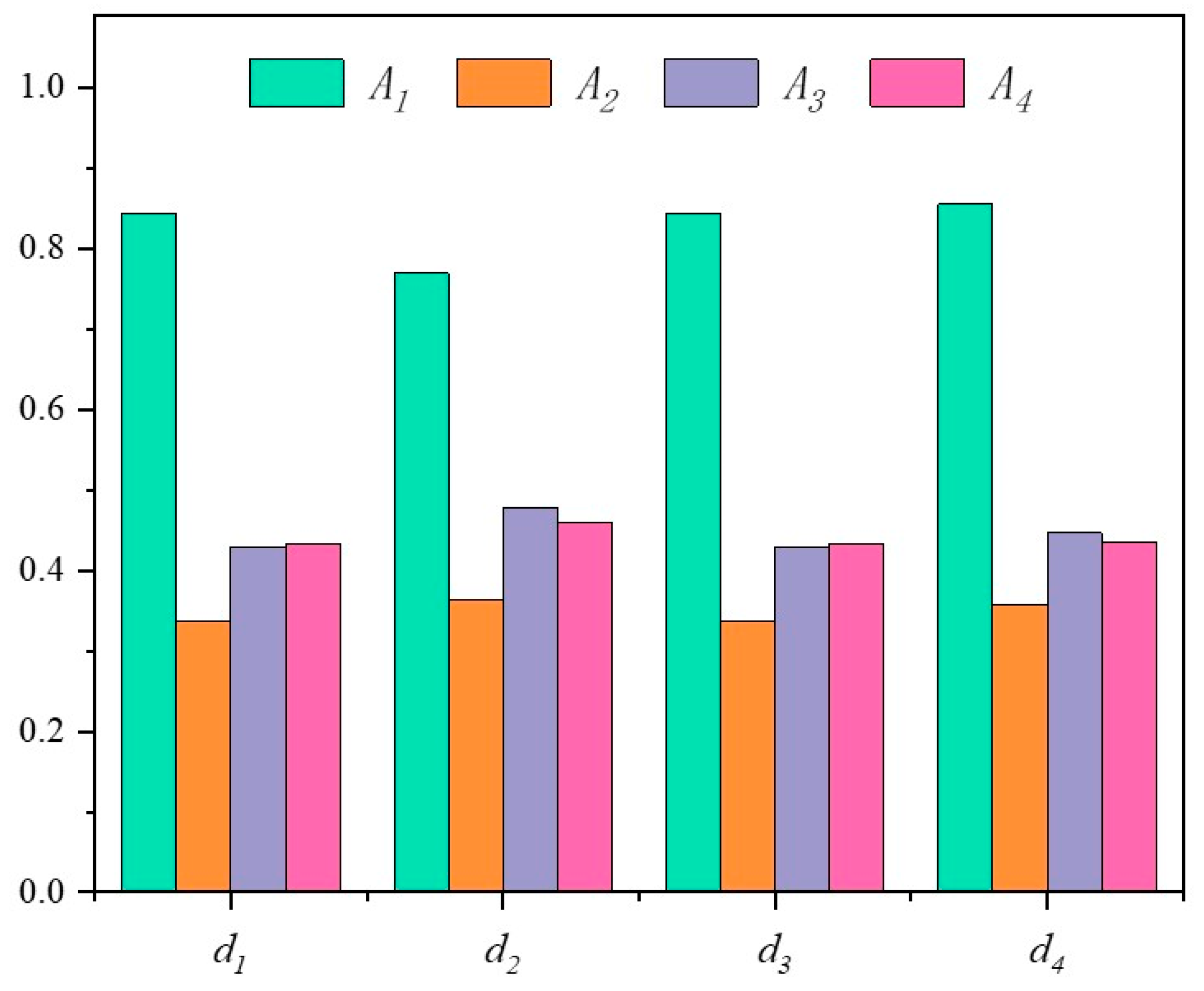
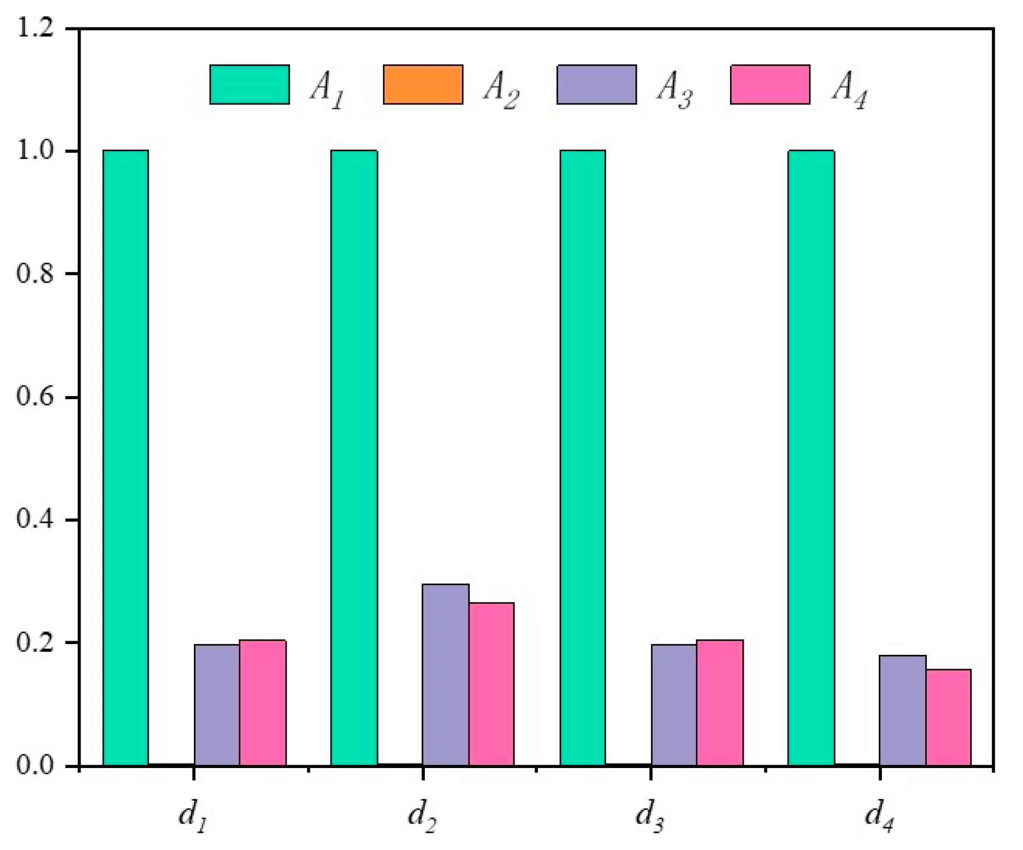
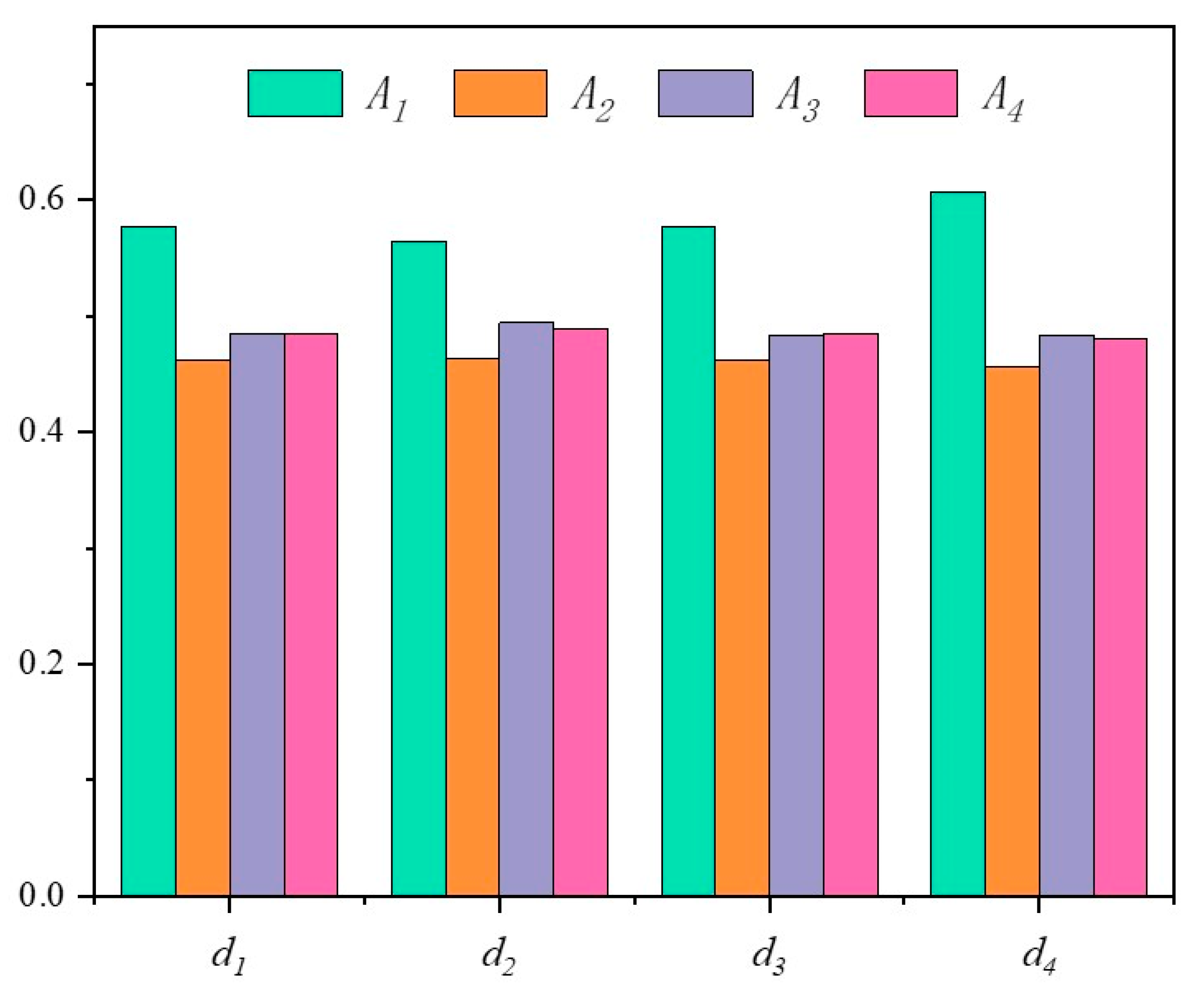
In view of this, the stability of the above results is analyzed through the four distance measures and three ranking methods mentioned above (see Figure 11, Figure 12 and Figure 13), as shown in

Table 8. Results of distance measures.

		A1	A2	A3	A4
d1	D(A,A+)	0.03517	0.15011	0.12696	0.12611
	D(A,A−)	0.18968	0.07630	0.09560	0.09645
d2	D(A,A+)	0.05468	0.16732	0.13444	0.13656
	D(A,A−)	0.18260	0.09535	0.12303	0.11595
d3	D(A,A+)	0.03516	0.15013	0.12699	0.12600
	D(A,A−)	0.18969	0.07632	0.09548	0.09646
d4	D(A,A+)	0.04340	0.19304	0.16600	0.16947
	D(A,A−)	0.25637	0.10775	0.13392	0.13089

and

Table 9. Results of ranking methods.

		A1	A2	A3	A4	Rank
C(Ai)	d1	0.84359	0.33702	0.42955	0.43336	A1 > A4 > A3 > A2
	d2	0.76956	0.36300	0.47783	0.45919	A1 > A3 > A4 > A2
	d3	0.84361	0.33703	0.42920	0.43361	A1 > A4 > A3 > A2
	d4	0.85523	0.35822	0.44652	0.43577	A1 > A3 > A4 > A2
RC(Ai)	d1	0	−3.8661	−3.1061	−3.0775	A1 > A4 > A3 > A2
	d2	0	−2.5379	−1.7851	−1.8625	A1 > A3 > A4 > A2
	d3	0	−3.8669	−3.1078	−3.0747	A1 > A4 > A3 > A2
	d4	0	−4.0280	−3.3029	−3.3947	A1 > A3 > A4 > A2
Sr(Ai)	d1	0.57777	0.46267	0.48413	0.48499	A1 > A4 > A3 > A2
	d2	0.56460	0.46343	0.49420	0.48953	A1 > A3 > A4 > A2
	d3	0.57778	0.46267	0.48406	0.48505	A1 > A4 > A3 > A2
	d4	0.60768	0.45645	0.48360	0.48027	A1 > A3 > A4 > A2

, and the data in Figure 12 have been normalized.

It can be seen from the analysis results that the best scheme obtained by changing the distance measures and ranking methods is still the MUH, so it can be considered that the results are accurate. In fact, in the actual production of Suichang Gold Mine, the application of this method has also achieved the ideal results of safety, efficiency and environmental protection.

Whether it can be considered that the model is universal and can be generalized in mining method optimization, the answer is obviously unknown. As is known, the factors that need to be considered in the optimization of mining methods are not completely fuzzy information, e.g., the recovery rate, cut ratio and other factors have certain empirical values. Therefore, the perfect solution is to build a corresponding transformation relationship between the exact value and the PFS and to build a mining method optimization model that combines fuzzy information with accurate data.

5. Conclusions

(1)

Through the PFS–TOPSIS method, based on the selection of technical and economic mining methods, a comprehensive evaluation system with multiple factors and indicators was constructed and an accurate closeness index was obtained to optimize mining methods. This overcomes the uncertainty and unpredictability of the traditional optimization system and provides a reference for the mining of the difficult-to-mine complicated orebody.

(2)

Taking Suichang Gold Mine as an example, according to the PFSTOPSIS method, a weighted aggregation evaluation matrix was constructed, and the closeness index of the four mining methods were calculated to be 0.8436, 0.3370, 0.4296 and 0.4334, respectively. The MUH has the highest closeness index, so this method was the best scheme.

(3)

There were many ranging methods and ranking methods for PFS and only one method could not ensure the accuracy and scientific nature of the results. This paper mainly used the first ranging method, which was ranked by the traditional closeness index. Finally, it discussed the three methods of traditional closeness index, revised closeness index and relative similarity values for comprehensive ranking under the four distance measures. When using the first distance measure, the revised closeness index of the four mining methods was 0, −3.8661, −3.1061 and −3.0775, and the relative similarity values were 0.5777, 0.46267, 0.48413 and 0.48499. It was concluded that MUH was the best scheme, which not only verified the accuracy of the results, but also showed that PFS was applicable to the selection of mining methods.

Of course, there are still limitations to the mathematical approach used in this study, i.e., indicators with definite values need to be evaluated first in natural language and then converted to fuzzy sets. Even so, the method still performs well in problems with a large amount of fuzzy information, such as the selection of mining methods. Therefore, we advocate the application of such methods to more mines and encourage more and more researchers to test and optimize them in practice.

References

1. Ma, D.; Duan, H.; Zhang, J.; Liu, X.; Li, Z. Numerical simulation of water-silt inrush hazard of fault rock: A three-phase flow model. Rock Mech. Rock Eng. 2022, 55, 5163–5182. [Google Scholar] [CrossRef]
2. Ma, D.; Duan, H.; Zhang, J. Solid grain migration on hydraulic properties of fault rocks in underground mining tunnel: Radial seepage experiments and verification of permeability prediction. Tunn. Undergr. Space Technol. 2022, 126, 104525. [Google Scholar] [CrossRef]
3. Ma, D.; Duan, H.; Zhang, J.; Bai, H. A state-of-the-art review on rock seepage mechanism of water inrush disaster in coal mines. Int. J. Coal Sci. Technol. 2022, 9, 50. [Google Scholar] [CrossRef]
4. Mijalkovski, S.; Peltechki, D.; Despodov, Z.; Mirakovski, D.; Adjiski, V.; Doneva, N. Methodology for underground mining method selection. Min. Sci. 2021, 28, 201–216. [Google Scholar] [CrossRef]
5. Ojha, M.; Singh, K.P.; Chakraborty, P.; Verma, S. A review of multi-objective optimisation and decision making using evolutionary algorithms. Int. J. Bio-Inspir. Comput. 2019, 14, 69–84. [Google Scholar] [CrossRef]
6. Saaty, T.L. What Is the Analytic Hierarchy Process? In Mathematical Models for Decision Support; Springer: Berlin/Heidelberg, Germany, 1988; pp. 109–121. [Google Scholar]
7. Jiskani, I.M.; Han, S.; Rehman, A.U.; Shahani, N.M. An Integrated Entropy Weight and Grey Clustering Method-Based Evaluation to Improve Safety in Mines. Min. Metall. Explor. 2021, 38, 1773–1787. [Google Scholar] [CrossRef]
8. Krishnan, A.R.; Kasim, M.M.; Hamid, R.; Ghazali, M.F. A Modified CRITIC Method to Estimate the Objective Weights of Decision Criteria. Symmetry 2021, 13, 973. [Google Scholar] [CrossRef]
9. Yang, W.G. Ingenious Solution for the Rank Reversal Problem of TOPSIS Method. Math. Probl. Eng. 2020, 2020, 9676518. [Google Scholar] [CrossRef] [Green Version]
10. Luo, D.; Wang, X. The multi-attribute grey target decision method for attribute value within three-parameter interval grey number. Appl. Math. Model. 2012, 36, 1957–1963. [Google Scholar] [CrossRef]
11. Omrani, H.; Alizadeh, A.; Naghizadeh, F. Incorporating decision makers’ preferences into DEA and common weight DEA models based on the best-worst method (BWM). Soft Comput. 2020, 24, 3989–4002. [Google Scholar] [CrossRef]
12. Yang, W.G.; Wu, Y.J. A New Improvement Method to Avoid Rank Reversal in VIKOR. IEEE Access 2020, 8, 21261–21271. [Google Scholar] [CrossRef]
13. Zhang, J.; Li, H.; Liu, Y.; Feng, X. The improvement and application of fuzzy comprehensive evaluation method under the hybrid information. In Proceedings of the 25th Chinese Control and Decision Conference (CCDC), Guiyang, China, 25–27 May 2013; p. 20131612-1615. [Google Scholar]
14. Samanta, S.; Jana, D.K. A multi-item transportation problem with mode of transportation preference by MCDM method in interval type-2 fuzzy environment. Neural Comput. Appl. 2019, 31, 605–617. [Google Scholar] [CrossRef]
15. Bera, A.K.; Jana, D.K.; Banerjee, D.; Nandy, T. A two-phase multi-criteria fuzzy group decision making approach for supplierevaluation and order allocation considering multi-objective, multi-product and multi-period. Ann. Data Sci. 2021, 8, 577–601. [Google Scholar] [CrossRef]
16. Karimnia, H.; Bagloo, H. Optimum mining method selection using fuzzy analytical hierarchy process–Qapiliq salt mine, Iran. Int. J. Min. Sci. Technol. 2015, 25, 225–230. [Google Scholar] [CrossRef]
17. Yavuz, M. The application of the analytic hierarchy process (AHP) and Yager’s method in underground mining method selection problem. Int. J. Min. Reclam. Environ. 2015, 29, 453–475. [Google Scholar] [CrossRef]
18. Guo, Q.Q.; Yu, H.X.; Dan, Z.Y.; Li, S. Mining Method Optimization of Gently Inclined and Soft Broken Complex Orebody Based on AHP and TOPSIS: Taking Miao-Ling Gold Mine of China as an Example. Sustainability 2021, 13, 12503. [Google Scholar] [CrossRef]
19. Iphar, M.; Alpay, S. A mobile application based on multi-criteria decision-making methods for underground mining method selection. Int. J. Min. Reclam. Environ. 2019, 33, 480–504. [Google Scholar] [CrossRef]
20. Atanassov, K.; Vassilev, P. Intuitionistic fuzzy sets and other fuzzy sets extensions representable by them. J. Intel. Fuzzy Syst. 2020, 38, 525–530. [Google Scholar] [CrossRef]
21. Bajic, S.; Bajic, D.; Gluscevic, B.; Vakanjac, V.R. Application of Fuzzy Analytic Hierarchy Process to Underground Mining Method Selection. Symmetry 2020, 12, 192. [Google Scholar] [CrossRef] [Green Version]
22. Memari, A.; Dargi, A.; Jokar, M.; Ahmad, R.; Abdul Rahim, A.R. Sustainable supplier selection: A multi-criteria intuitionistic fuzzy TOPSIS method. J. Manuf. Syst. 2019, 50, 9–24. [Google Scholar] [CrossRef]
23. Narayanamoorthy, S.; Geetha, S.; Rakkiyappan, R.; Joo, Y.H. Interval-valued intuitionistic hesitant fuzzy entropy based VIKOR method for industrial robots selection. Expert Syst. Appl. 2019, 121, 28–37. [Google Scholar] [CrossRef]
24. Yager, R.R. Pythagorean Membership Grades in Multicriteria Decision Making. IEEE Trans. Fuzzy Syst. 2014, 22, 958–965. [Google Scholar] [CrossRef]
25. Peng, X.D.; Selvachandran, G. Pythagorean fuzzy set: State of the art and future directions. Artif. Intel. Rev. 2019, 52, 1873–1927. [Google Scholar] [CrossRef]
26. Akram, M.; Dudek, W.A.; Ilyas, F. Group decision-making based on pythagorean fuzzy TOPSIS method. Int. J. Intel. Syst. 2019, 34, 1455–1475. [Google Scholar] [CrossRef]
27. Yager, R.R. Pythagorean Fuzzy Subsets. In Proceedings of the Joint World Congress of the International-Fuzzy-Systems-Association (IFSA)/Annual Meeting of the North-American-Fuzzy-Information-Processing-Society (NAFIPS), Edmonton, AB, Canada, 24–28 June 2013; p. 201357-61. [Google Scholar]
28. Yager, R.R.; Abbasov, A.M. Pythagorean Membership Grades, Complex Numbers, and Decision Making. Int. J. Intel. Syst. 2013, 28, 436–452. [Google Scholar] [CrossRef]
29. Zhang, X.L.; Xu, Z.S. Extension of TOPSIS to Multiple Criteria Decision Making with Pythagorean Fuzzy Sets. Int. J. Intel. Syst. 2014, 29, 1061–1078. [Google Scholar] [CrossRef]
30. Zhang, X.L. A Novel Approach Based on Similarity Measure for Pythagorean Fuzzy Multiple Criteria Group Decision Making. Int. J. Intel. Syst. 2016, 31, 593–611. [Google Scholar] [CrossRef]
31. Hwang, C.L.; Yoon, K. Methods for Multiple Attribute Decision Making. In Multiple Attribute Decision Making; Springer: Berlin/Heidelberg, Germany, 1981; pp. 58–191. [Google Scholar]
32. Wu, Z.; Li, Q.; Kong, D.; Chen, G.; Luo, D. The ANP-Fuzzy-TOPSIS model for the optimization of the scheme of large-section blasting. Arab. J. Geosci. 2020, 13, 1–9. [Google Scholar] [CrossRef]
33. Feasibility Study Report on Safe, Efficient and Low Lean Filling Mining of High Grade Gold and Silver Resources in Soft Rock Strata; Central South University: Changsha, China, 2021.
34. Yu, H.X.; Li, S.; Yu, L.F.; Wang, X. The Recent Progress China Has Made in Green Mine Construction, Part II: Typical Examples of Green Mines. Int. J. Environ. Res. Public Health 2022, 19, 8166. [Google Scholar] [CrossRef]
35. Ejegwa, P.A.; Awolola, J.A. Novel distance measures for Pythagorean fuzzy sets with applications to pattern recognition problems. Granular Comput. 2021, 6, 181–189. [Google Scholar] [CrossRef]
36. Mahanta, J.; Panda, S. Distance measure for Pythagorean fuzzy sets with varied applications. Neural Comput. Appl. 2021, 33, 17161–17171. [Google Scholar] [CrossRef]
37. Ejegwa, P.A. Distance and similarity measures for Pythagorean fuzzy sets. Granular Comput. 2020, 5, 225–238. [Google Scholar] [CrossRef]
38. Hussian, Z.; Yang, M.S. Distance and similarity measures of Pythagorean fuzzy sets based on the Hausdorff metric with application to fuzzy TOPSIS. Int. J. Intel. Syst. 2019, 34, 2633–2654. [Google Scholar] [CrossRef]
39. Hadi-Vencheh, A.; Mirjaberi, M. Fuzzy inferior ratio method for multiple attribute decision making problems. Inform. Sci. 2014, 277, 263–272. [Google Scholar] [CrossRef]
Figure 1. Plan of 140–260 m middle section of Suichang Gold Mine.
Sustainability 15 03692 g001
Figure 2. Spatial comparison between PFS and other fuzzy sets.
Sustainability 15 03692 g002
Figure 3. Framework of PFS-TOPSIS method.
Sustainability 15 03692 g003
Figure 4. Plan of the Suichang gold mine (accessed on 10 July 2022. https://www.fengyunditu.com/?ver=bd-wx-1604).
Sustainability 15 03692 g004
Figure 5. Construction of green mine at SuiChang gold mine: (a) exterior view of SuiChang National Mine Park; (b) the gold grottoes of the Dang Dynasty; (c) the gold grottoes of the Song Dynasty; (d) mining disaster size from the Ming Dynasty [29]. (cc by-sa 4.0).
Sustainability 15 03692 g005
Figure 6. Mining method diagram of MUH.
Sustainability 15 03692 g006
Figure 7. Mining method diagram of GUH.
Sustainability 15 03692 g007
Figure 8. Mining method diagram of UHA.
Sustainability 15 03692 g008
Figure 9. Mining method diagram of SFM.
Sustainability 15 03692 g009
Figure 10. Mechanized mining in the Suichang gold mine: (a) filling material; (b) filling station; (c) resource survey; (d) mechanized mining [34]. (cc by-sa 4.0).
Sustainability 15 03692 g010
Figure 11. Closeness index rank based on different distance measures.
Sustainability 15 03692 g011
Figure 12. Revised closeness index rank based on different distance measures.
Sustainability 15 03692 g012
Figure 13. Relative similarity values rank based on different distance measures.
Sustainability 15 03692 g013