Article

Hydrological Modeling of the Kobo-Golina River in the Data-Scarce Upper Danakil Basin, Ethiopia

1
State Key Laboratory of Hydraulic Engineering Simulation and Safety, School of Civil Engineering, Tianjin University, Tianjin 300350, China
2
Amhara Design and Supervision Works Enterprise, Bahir Dar P.O. Box 1921, Ethiopia
3
Faculty of Civil and Water Resources Engineering, Bahir Dar Institute of Technology, Bahir Dar University, Bahir Dar P.O. Box 26, Ethiopia
4
Hydrological Science Group, Department of Land, Air, and Water Resources, University of California, Davis One shield Avenue, Davis, CA 95616, USA
*
Author to whom correspondence should be addressed.
Sustainability 2023, 15(4), 3337; https://doi.org/10.3390/su15043337
Submission received: 23 December 2022 / Revised: 3 February 2023 / Accepted: 7 February 2023 / Published: 11 February 2023

Abstract

:
A proper understanding of hydrological processes is vital for water resource assessment, management, and conservation at a local, national, and global scale. The role of hydrological models is critically important in rarely studied ungauged catchments including of Kobo-Golina, in the Danakil basin of Ethiopia. The main objective of this research is to model the hydrology of the Kobo-Golina catchment using the completely restructured SWAT (SWAT+) model. Validated reanalysis river flow from the Global Flood Awareness System (GloFAS) and actual evapotranspiration (AET) from Moderate Resolution Imaging Spectroradiometer (MODIS) were used for single and multi-variable calibration. It is found that the multi-variable calibration scenario reasonably attained the minimum satisfactory performance limit for both variables (NSE = 0.67, R2 = 0.68, PBias = −9.68%, and RSR = 0.57 for calibration of GloFAS flow; and NSE = 0.56, R2 = 0.63, RSR = 0.66, PBias = 3.86 for calibration of MODIS AET). The model simulation showed that evapotranspiration accounts for 47% of the input water while surface runoff, lateral flow, and groundwater recharge account for 30%, 1.53%, and 21.4%, respectively. The simulated mean annual streamflow at the Basin outlet is 10.6 m3/s. The monthly low flow occurs in June with a median flow of 1.43 m3/s and a coefficient of dispersion of 0.67. High flows occur in August, with a median flow of 16.55 m3/s and a coefficient of dispersion of 1.55. The spatial distribution of simulated runoff was depicted as being higher in the floodplains and along the riparian/drainage lines, whereas upland areas showed lower runoff. The maximum monthly recharge occurs in September with a recharge value of 78.2 mm. The findings of the study suggested that both surface water harvesting and groundwater exploitation can be sought in floodplain areas while conserving the uplands.

1. Introduction

Water is one of the most vital and core resources for sustainable development around the globe [1]. Its role in socio-economic, and environmental development aspects is priceless. At this time, the world’s population is increasing at an alarming rate, putting a strain on water resources in a variety of ways [2]. Unless special attention is paid to the sustainable use of water resources, it will be a great global risk [3]. It is concerning that the current water use, particularly in Ethiopia, is not wise considering the exploitable potential of available water resources [4,5].
According to recent surveys, about 65% of the world’s population experiences severe water scarcity for at least one month per year [6]. Currently, more than two billion people live in countries with insufficient water supply [7]. Fifty percent of the world’s population could be living in water-stressed areas by as early as 2025 [6]. Ethiopia has a population of about 120 million people [8] and has immense water resources [9]. However, spatial and temporal variability of rainfall has caused water scarcity in many parts of the country [10]. Nearly 27 million of Ethiopia’s population lives in areas of high water stress [11]. Though rainfed agriculture contributes significantly to Ethiopia’s economy, its variability is the source of water stress and chronic food insecurity [12,13].
The current study area, the Kobo-Golina basin, is one of the drought-prone areas in the country due to erratic rainfall [14,15]. The area is identified as one of the potential areas for surface and groundwater irrigation [16]. Both surface and groundwater irrigation have been practiced in the basin since 1999 [16,17,18]. The government is planning to expand the number of irrigation projects in the country including this area in the coming years [19].
Though irrigation is under development, the area is facing some problems like poor water management [16,17,20] and a lack of sufficient hydrological information [21]. Water balance components are not properly defined. Random utilization of resources without understanding the hydrology of the area is still a challenge. So, scientific intervention is required to understand hydrology and assess the potential to properly manage the water resource of the area. Hydrological quantification of water resources, simulation, and monitoring of the water balance components are critical for the area. This will help to properly understand the potential and mitigate the problems in utilizing the resources. Hydrological models are among the various tools used to quantify and predict changes in the spatial and temporal availability as well as the quality of water resources [22]. Due to its improved features, multiple internal processes, and versatility [23,24], the SWAT model is widely applicable globally. The application of the SWAT model for the study of water resources and environmental assessments has shown significant progress in Africa [25]. The SWAT model application in Ethiopia is also progressive but limited to a few major river basins which have ground-measured data [26,27,28,29,30]. Hydrological modeling through SWAT is rare in ungauged basins due to a lack of data. There is not a significant number of studies that focused particularly on data-scarce humid and semi-arid regions including the current study area. The SWAT model has never been applied before in the Kobo-Golina River to simulate the hydrological characteristics of the watershed.
Recent studies indicated that the humid and semi-humid tropical highlands of Ethiopia showed a saturation excess runoff process [31]. For this, SWAT+ was recently developed to separate upland and floodplain regions to better simulate lowland hydrology—saturation excess runoff [32]. SWAT+ will be applied for the hydrological simulation of the Kobo-Golina catchment as the majority of the area is humid. However, the availability of input and calibration data is still a constraint. At this time, open-source remote sensing technologies are offering alternative input data and simplifying the application of the SWAT model [33,34]. A prior study has not been performed to assess the hydrology of this watershed using SWAT+ and open-source remote sensing data. The novelty of this research then, is the use of open sources remotely sensed data and the application of the recent SWAT+ to generate data/information on the hydrology of the ungauged Kobo-Golina catchment. According to our knowledge, this research work is the first of its kind in the humid and semi-arid regions of the Danakil Basin in Ethiopia. The outputs from this research are of great scientific importance and provide supplemental information on streamflow in data-scarce areas of the Kobo-Golina catchment in the Danakil Basin of Ethiopia.
The main objective of this research is then to model the hydrology of the Kobo-Golina catchment by SWAT+ using open-source remote sensing data. First, single and multi-variable calibration approaches were applied to simulate hydrologic processes; second, water balance components, water yield, and total water storage were assessed; finally, groundwater recharge has been characterized. The major advantage of the proposed methodology is that it has been developed for typical ungauged humid and semi-arid hydrological regimes in the Danakil Basin of Ethiopia and can be easily applied to catchments with similar hydrological and geomorphological characteristics. Such an approach provides vital information and insights to improve understanding of the hydrological processes of ungauged catchments in humid and semi-arid hydrological regions.

2. Materials and Methods

2.1. Study Area

The Kobo-Golina sub-basin is located in the Northeast part of the Amhara region in Northern Ethiopia. It is located in the upper part of the Danakil Basin. It is geographically extending from 11°55′33.6″ to 12°14′20.4″ N latitude and 39°22′30″ to 39°49′44.4″ E longitude. The area has a humid and semi-arid climate in the hills and valley plains, respectively. It covers an estimated drainage area of 1040 km2 at an outlet of the Golina River (Figure 1). The elevation of the area varies from 1117 to 3972 m and with a mean elevation of 1971 m. The study area receives a mean annual rainfall of 727 mm (2003–2005) and has a bi-modal type of rainfall. The long rainy season occurs from June to mid September and the short rainy season from March to April. The average monthly temperatures of the study area range from 18.7 °C in December to about 26 °C in June. The dominant soil in the study area is vertisol and leptosol. The major annual crop types grown under rain-fed cultivation are sorghum, teff, and maize.

2.2. Data Sources and Description

The basic data required and used in the study are (i) insitu rainfall and streamflow data for validation of reanalysis rainfall and GloFAS streamflow, respectively; (ii) Climate data: CHIRPS precipitation, CFSR temperature, relative humidity, solar radiation, wind speed along with spatial data: DEM, Land use/Landcover and soil for model input; (iii) MODIS evapotranspiration (MOD16A2 8 days) and reanalysis GloFAS stream flow data for calibration and validation of the model.

2.2.1. Hydro-Meteorological Data

Climate Data

There are three meteorological stations found within the watershed area (i.e., Kobo, Tekulesh, and Zobel). They have records of rainfall and temperature for different periods having missed data exceeding 40%. As a result, reanalysis data were considered as an alternative source of data to fill the gap. CHIRPS rainfall is recommended as an alternative source of rainfall data in ungauged catchments of Ethiopia [27,35,36]. Scatterplot and correlation coefficient review of open-access precipitation products such as CFSR, ERA5, and CHIRPS also confirmed that CHIRPS had the best performance of all [37].
The daily maximum and minimum temperature, daily relative humidity, solar radiation, and wind speed found within the SWAT+ CSFR-World weather generator were used to simulate the model [27,36,38].

Hydrological Data

Conventionally, the SWAT model is calibrated based on measured streamflow data from hydrometeorological stations [24,36,39,40]. However, there is no sufficient streamflow data in the study area. The only streamflow gauging station located in the study area is the Golina weir site (upstream of the main outlet). The station was operational for a short period (1979–1983) with several missed data. This data is not sufficient to calibrate the model but is used for the validation of remote sensing streamflow data. The validated streamflow data is then employed for calibration of the SWAT model.

2.2.2. Spatial Data for Model Input

DEM, Land Use, and Soil

The watershed delineation and the streamflow networks extraction were performed based on 30 m resolution SRTM Digital elevation model (DEM). The subbasins were further discretized into basic computational units called Hydrologic Response Units (HRUs). Slope, 10 m resolution ESRI Sentinel-2 Land Use/Land Cover data [41], and African Soil Information System soil data (AFSIS) [42] were used to discretize the subbasins into HRU. DEM, Land use land cover and soil map of the study area are presented in Figure S1 in Supplementary Materials. All datasets utilized in the study are summarized in Table 1.

Reanalysis GloFAS River Discharge Dataset

Considering the lack of measured streamflow data, satellite-based/reanalysis stream flow was introduced recently with various time steps and resolution; the Global Flood Awareness System (GloFAS) is one of these products which provides reanalysis river flow estimates at a worldwide scale since 1979 [43]. GloFAS data has substantial potential for calibrating the SWAT hydrological model in the ungauged watersheds of the Grande San Miguel River Basin (El Salvador) [44]. This study recommended the application of GloFAS flow for water resource management studies for similar un-gauged catchments [44]. Additionally, GloFAS streamflow data was validated using measured streamflow data before use in the model. Considering this fact, the validated GloFAS stream flow data (1997–2021) with monthly time steps and 0.1° spatial resolution was used for calibration and validation of the model.

Remotely Sensed AET

Beyond its scarcity, calibrating hydrological models against only simulated hydrograph (Streamflow data) can lead to parameter equifinality [45,46,47]. This will result in low simulation accuracy of hydrological variables like evapotranspiration and groundwater [48,49]. Evapotranspiration has a major share (>60%) of the global average water budget and influences the water balance of the system [50]. Model parameterization for streamflow calibration significantly affects the simulation of actual evapotranspiration and vice versa [50,51,52]. As a result, it is very reasonable and beneficial to use AET for calibration and validation of the hydrological model [53].
Observed AET data is not available across Ethiopia [54]. Remote sensing AET data such as MODIS AET and AVHRR (Advanced Very High-Resolution Radiometer) AET are recommended as alternative data for the calibration of SWAT [54]. Based on this recommendation, the Moderate Resolution Imaging Spectrometer (MOD16 AET) 250 m resolution data for the years 2001–2021 was used for calibration and validation of the model.
Table 1. Data type, source, and intended use in the study.
DataDescriptionSourcesUse
Meteorological DataDaily station data of rainfall (2003–2005)Ethiopian National Meteorological Services Agency
https://www.ethiomet.gov.et (accessed on 1 September 2022)
For validation of CHIRPS precipitation data
Hydrological DataStreamflow data (1979–1982)Ethiopian Ministry of Water and EnergyFor validation of GloFAS river flow
TopographyDigital elevation model (DEM) 1 arc-second for global coverage (~30 m)https://earthexplorer.usgs.gov/ (accessed on 15 September 2022)SWAT+ watershed delineation
Soil250 m resolution, soil property maps of AfricaSoil property maps of Africa (AFSIS, 2015; [42]
https://www.isric.org/projects/soil-property-maps-africa-250-m-resolution (accessed on 1 October 2022)
SWAT+ HRU definition
Land use10 m resolution ESRI Sentinel-2 Land Use/Land Coverhttps://livingatlas.arcgis.com/landcover/ (accessed on 16 October 2022)SWAT+ HRU definition
Reanalysis climate data-CHIRPS Reanalysis rainfall data with daily time step and a resolution of 0.05° × 0.05°
-CFSR Reanalysis climate data with daily time steps and a resolution of 0.30° × 0.30°
https://data.chc.ucsb.edu/products/CHIRPS-2.0/ (accessed on 1 November 2022)
https://globalweather.tamu.edu/ (accessed on 28 October 2022
Input for SWAT+
Reanalysis River dischargeGloFAS River Discharge Reanalysis Dataset with daily time steps and 0.1° spatial resolutionhttps://cds.climate.copernicus.eu, (accessed on 5 November 2022SWAT+ model Simulation calibration and validation
Remotely sensed
based Actual
Evapotranspiration
(AET)
Moderate Resolution Imaging Spectrometer (MOD16A2 8 Day) available at 500 m resolution; [55]https://modis.gsfc.nasa.gov/data/dataprod/mod16.php (accessed on 20 November 2022)SWAT+ model simulation calibration and validation

2.3. SWAT Model Description and Setup

In this study, SWAT+ version 2.1.10 was used. QSWAT+, which is the QGIS (Quantum GIS) interface for SWAT+, owns various QGIS functionalities and provides a more flexible spatial representation of interactions and processes [32]. SWAT+ with landscape unit (LSU) option was selected to discretize subbasins to allow separation of upland processes from wetlands [32].
30 × 30 m SRTM DEM was employed to delineate the watershed. 6 km2 and 60 km2 were considered as channel and stream area thresholds, respectively. Discretization of the model provided 9 subbasins and 696 HRUs. HRU thresholds of 20% for land use, 10% for soil type, and 20% for slope were applied (Table 2). DEM inversion method was used to create LSU (Figure S2). The area of the subbasin generated ranges from 0.61 km2 to 135 km2. SWAT+ Editor 2.0.4 was utilized to set up the project, edit SWAT+ inputs, run the model, and check the QSWAT+ model.
Potential evapotranspiration was estimated using the Penman–Monteith equation [56]. The Penman–Monteith method requires air temperature, solar radiation, relative humidity, and wind speed as input in Equation (1):
λ E = X ( H n e t G ) + ρ a i r X C p X ( e z o e z ) / r a + γ X ( 1 + r c r a )  
where λ is the latent heat flux density (MJ m−2 day−1), E is the depth rate evaporation (mm day−1), △ is the slope of the saturation vapor pressure-temperature curve, de = dT (kPa °C−1), Hnet is the net radiation (MJ m−2 day−1), G is the heat flux density to the ground (MJ m−2 day−1), ρair is the air density (kg m−3), Cp is the specific heat at constant pressure (MJ kg−1 °C−1), e z o is the saturation vapor pressure of air at height z (kPa), ez is the water vapor pressure of air at height z (kPa), γ is the psychrometric constant (kPa °C−1), rc is the plant canopy resistance (s m−1), and ra is the aerodynamic resistance (s m−1).
The Soil Conservation Service’s Curve Number method was employed to estimate the surface runoff. Surface runoff was estimated separately for each HRU and routed to the outlet of a subbasin to make the cumulative runoff of the subbasin. The Muskingum routing method was used to route the streamflow within the subbasin channels. Finally, model simulations were performed at a daily time step from 1991 to 2021. The three-year warm-up period was considered to run the model.

2.4. Sensitivity Analysis

Sensitivity analysis, calibration, and validation of model parameters were carried out using SWAT+ TOOLBOX Version 0.7.6 [57]. SWAT+ TOOLBOX is an independent tool from SWAT+. The initial model parameters were selected referring to the existing literature [40,58,59]. 13 parameters were selected and first-order sensitivity analysis was performed related to (i) MODIS AET only and GloFAS flow only scenario separately and (ii) both AET and GloFAS flow concurrently using Variance-based sensitivity analysis (Sobol) method. The Sobol method is the widely applicable method that is relatively reliable for quantifying sensitivity and ranking parameters based on p-factor and t-test [60]. It deals with nonlinear responses, and it can measure the effect of interactions in non-additive systems [61]. 1300 seed was selected to run 36,400 samples until the most sensitive parameters were attained. Parameters that have sensitivity values of zero were supposed to be removed but decided to remain there considering their importance for further fine-tuning in other models. The description of the SWAT parameters, change type, and their minimum and maximum range are presented in Table S1 in Supplementary Materials.

2.5. Model Calibration and Validation

Following the sensitivity analysis, model calibration was performed using both GloFAS flow and MODIS AET at the monthly time step. Model calibration and validation were performed from the year 2001–2011 and 2012–2014, respectively. Data after 2014 were not considered because of disturbed natural flow conditions due to intensive irrigation.
Two calibration strategies were investigated. First, single-variable calibration was considered. In the single variable calibration scenario, parameters were calibrated based on GloFAS flow at the main outlet and MODIS AET at the entire basin separately. Finally, SWAT model parameters were calibrated/validated in the multi-variable calibration scenario employing both MODIS AET and GloFAS flow concurrently.

2.6. Model Performance Evaluation and Verification

The objective function used during the calibration and validation in all scenarios was the Nash–Sutcliffe efficiency (NSE) on Equation (2) [58]. Evaluation of the model performance is greatly affected by the choice of a particular statistical ‘‘goodness-of-fit’’ [62]. In addition to NSE, coefficient of determination (R2) on Equation (3), RSR (the ratio of root means square error (RMSE) to the standard deviation of the measured data) on Equation (4), and percent bias (PBias) on Equation (5) were also considered to eliminate subjectivity in assessment of the model performance.
NSE = 1 i = 1 N ( S i O i ) 2 i = 1 N ( O i O mean ) 2
R 2 = ( i = 1 N ( O i O mean ) ( S i S mean ) i = 1 N ( O i O mean ) 2 i = 1 N ( S i S mean ) 2 ) 2
RSR = i = 1 N ( S i O i ) 2 i = 1 N ( O i O mean ) 2
PBias = 100   ×   i = 1 N ( O i S i ) i = 1 N O i
where S = Model Simulated output; O = observed hydrological variable; Omean = mean value of the observations that the NSE uses as a benchmark against which the performance of the model is compared; and N = number of observations. NSE values range from—∞ to 1, where 1 shows a perfect model. If NSE is zero, it implies that the observed mean is as good a predictor as the model, and if NSE is less than zero to negative infinity, then the model is a worse predictor than Qmean. NSE > 0 is considered a generally accepted agreement between subject variables; whereas, NSE > 0.5, R2 > 0.5, RSR ≤ 0.7, and PBias ± 25% are considered satisfactory values [63,64].
Relying solely on performance indicator values (NSE, R2, RSR, PBias) will not ensure that the model performs well. Qualitative evaluation was also assessed through a graphical comparison of model-simulated variables with that of satellite-based AET and GloFAS river flow within the calibration and validation period.

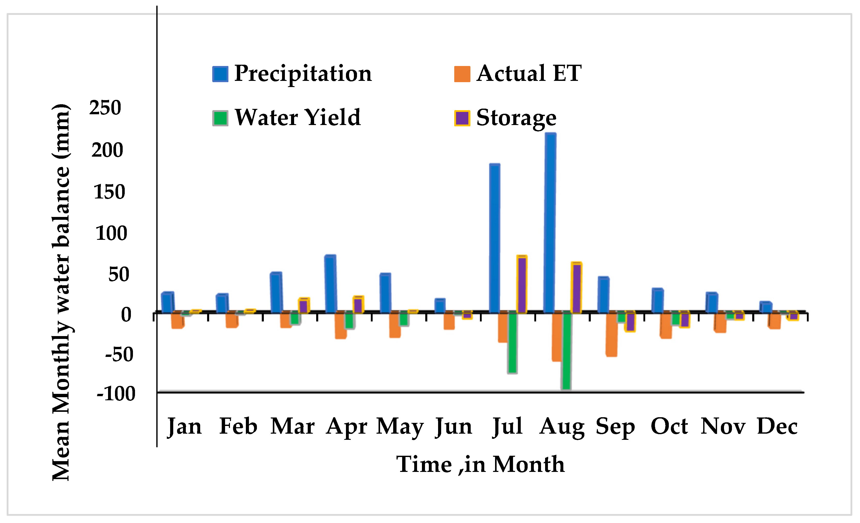
2.7. Water Balance, Water Yield, and Total Water Storage Assessment

An assessment of the long-term average water balances of the watershed was carried out based on SWAT+ simulated output. The water yield of the catchment is predicted using the following equation.
Water Yield (WY) = SURQ + LATQ+ Qgw/Perc − Tloss
where
  • SURQ is the surface runoff;
  • LATQ is the lateral flow;
  • Qgw/Percolation is the groundwater contribution to streamflow;
  • Tloss is the transmission loss.
Total water storage (WS) is also analyzed to see whether there is excess or deficit of water in the catchment for the given month. Either release or storage of water is expected for different months. Water storage is calculated by deducting runoff and AET from precipitation. Two cases are considered to see the water storage condition of the basin:
Case (i) If PCP (Precipitation) > WY + AET (Positive storage), excess water infiltrated and stored as soil moisture and groundwater (GW) storage.
Case (ii) If PCP (Precipitation) < WY + AET (Negative storage), implying water deficit will be compensated from the storage.

3. Result and Discussion

3.1. Correlation of Observed and Reanalysis Datasets

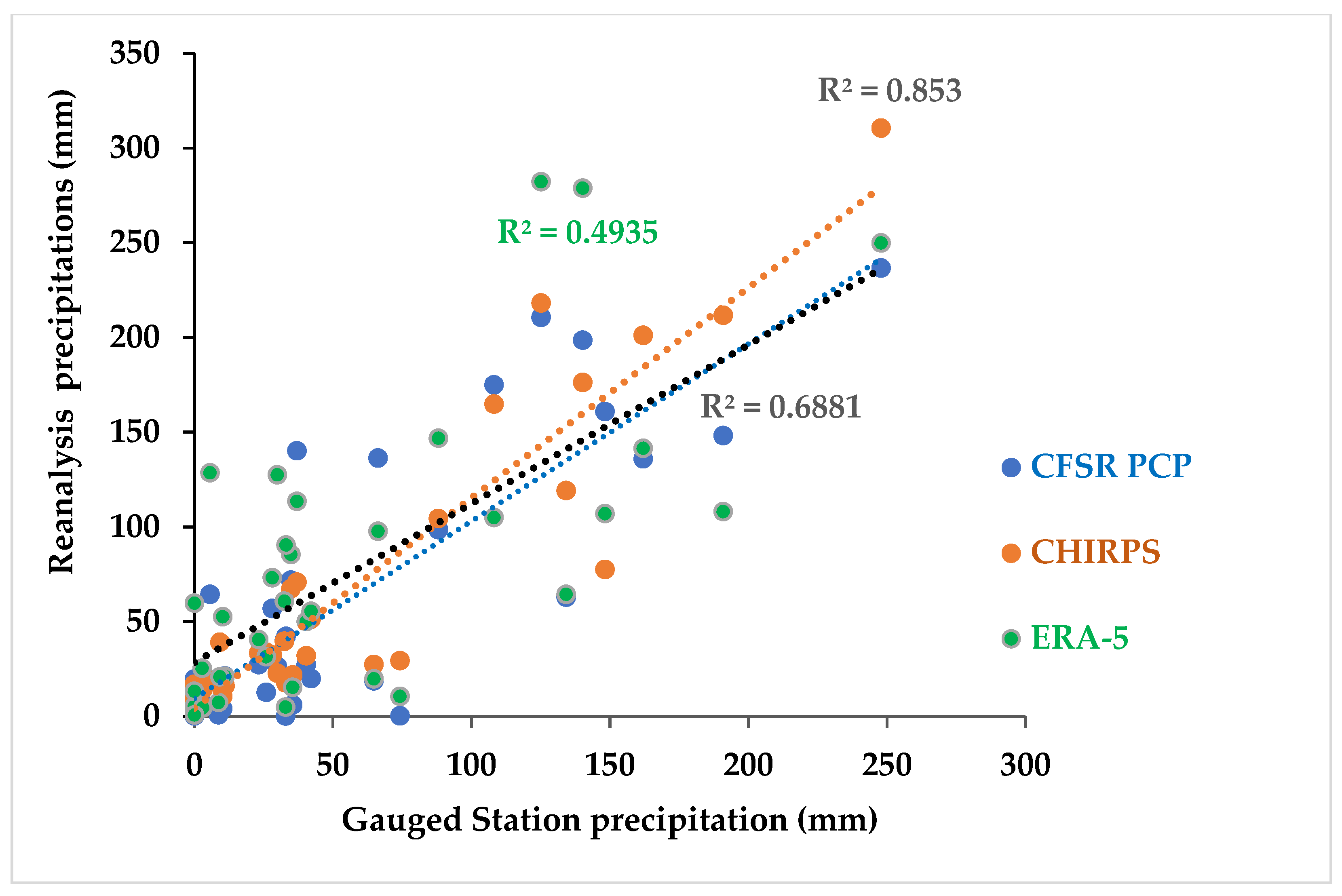
3.1.1. Correlation of Rain Gauge Station and Reanalysis Precipitation Data

A correlation coefficient was determined between measured rainfall from the Kobo station and open-source reanalysis rainfall (CHIRPS, ERA5, and CFSR) for the same period. Figure 2 depicts that CHIRPS reanalysis rainfall has a better correlation efficiency of 85% (R2 = 0.85) than the other two (ERA5 and CFSR). A scatterplot of the CHIRPS and observed rainfall points were spread relatively close to the 45° line, indicating a better agreement between the two datasets. Finally, CHIRPS rainfall was used as input climate data in the model.
A study conducted by [65] in North Wollo, including the Kobo area, showed that CHIRPS rainfall has a strong correlation with observed rainfall. The authors of [66] also validated CHIRPS rainfall in the Zeway basin of Ethiopia and has a good correlation. Other studies in the upper Blue Nile Basin of Ethiopia by [27,35] confirmed that CHIRPS rainfall is suitable and performs well in the SWAT model simulation. A study by [67] in the Tekeze basin of Ethiopia also confirmed CHIRPS rainfall as it is suitable and performs well in the simulation of the SWAT hydrological model.

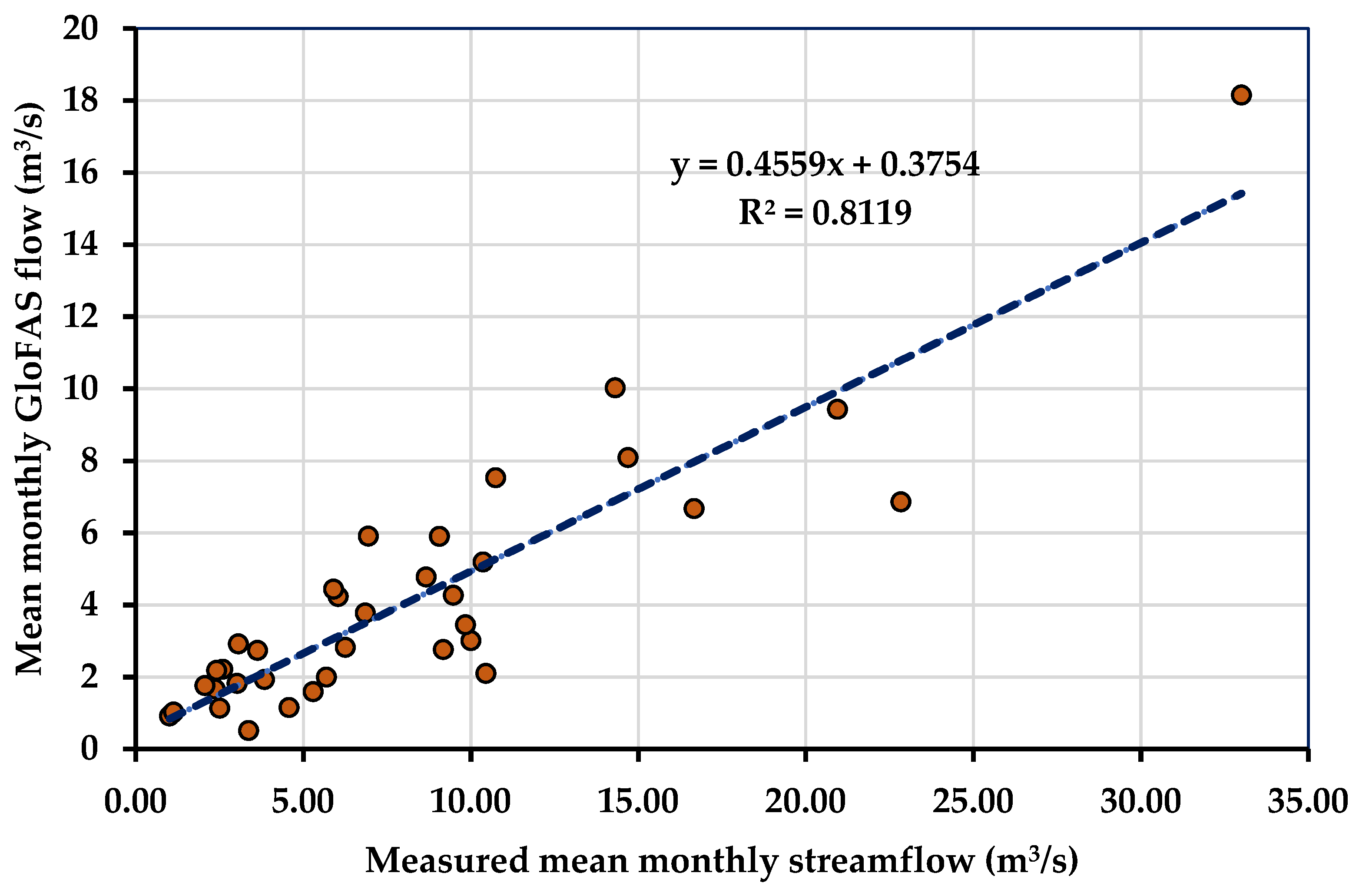
3.1.2. Correlation of Measured Streamflow and Reanalysis GloFAS Flow

A correlation coefficient was determined between GloFAS flow and measured streamflow at the Golina weir site. The correlation showed a reasonably good result, R2 = 0.82 (Figure 3). As a result, GloFAS flow was employed for model calibration. A scatterplot of the GloFAS flow and observed streamflow points were spread close to the 45° line, indicating a better agreement between the two datasets.

3.2. SWAT Model Performance

3.2.1. Default Analysis

Tthe NSE, R2, RSR, and PBias values at default model run depict a low performance according to [63,64]. The results of the default run support the need to improve the SWAT model’s performance further. As a result, the SWAT model outputs were subjected to further calibration and validation.

3.2.2. Sensitivity Analysis

The common parameters found to be sensitive in all circumstances were runoff curve number (CN2.hru), the available water capacity of the soil layer (sol_awc), and Percolation coefficient (perco.hru). When considering GloFAS flow alone and multi-variable simulation, CN2 was the first highly sensitive parameter to demonstrate substantial effects, whereas, in the case of simulation of AET only, an available water capacity of the soil layer (sol_awc) was the first most sensitive parameter.
Similar results were obtained in the Chindwin Basin of Myanmar [68] in which CN2 was the most sensitive model parameter for streamflow and multivariable simulation scenario, and SOL_AWC was the most sensitive model parameter for evapotranspiration. Another study conducted in the Grande San Miguel River Basin (El Salvador) [44] coincides with the findings of this study that CN2 was the most sensitive parameter in GloFAS flow-based SWAT model calibration. Table 3 displays the lists of calibrated model parameters, change procedures, and calibrated values.

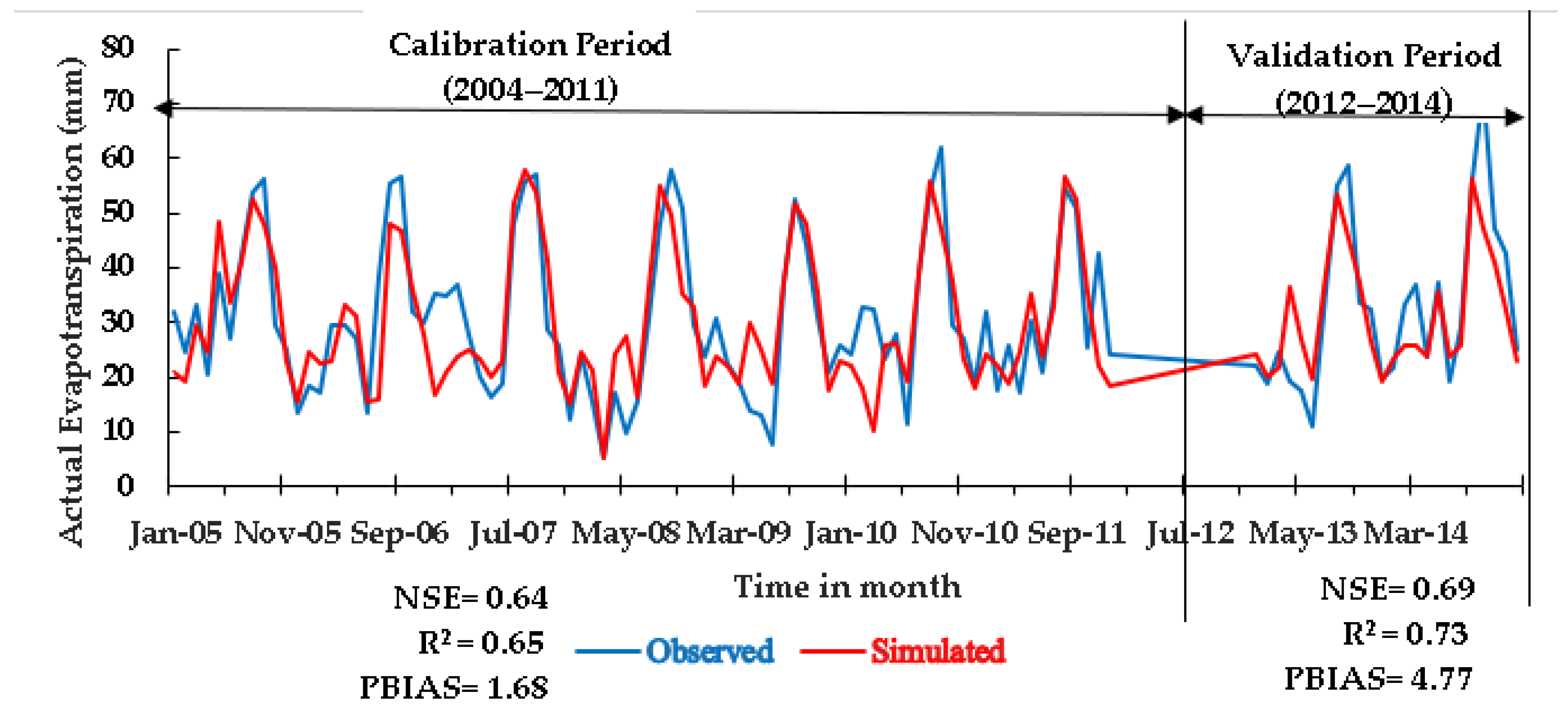
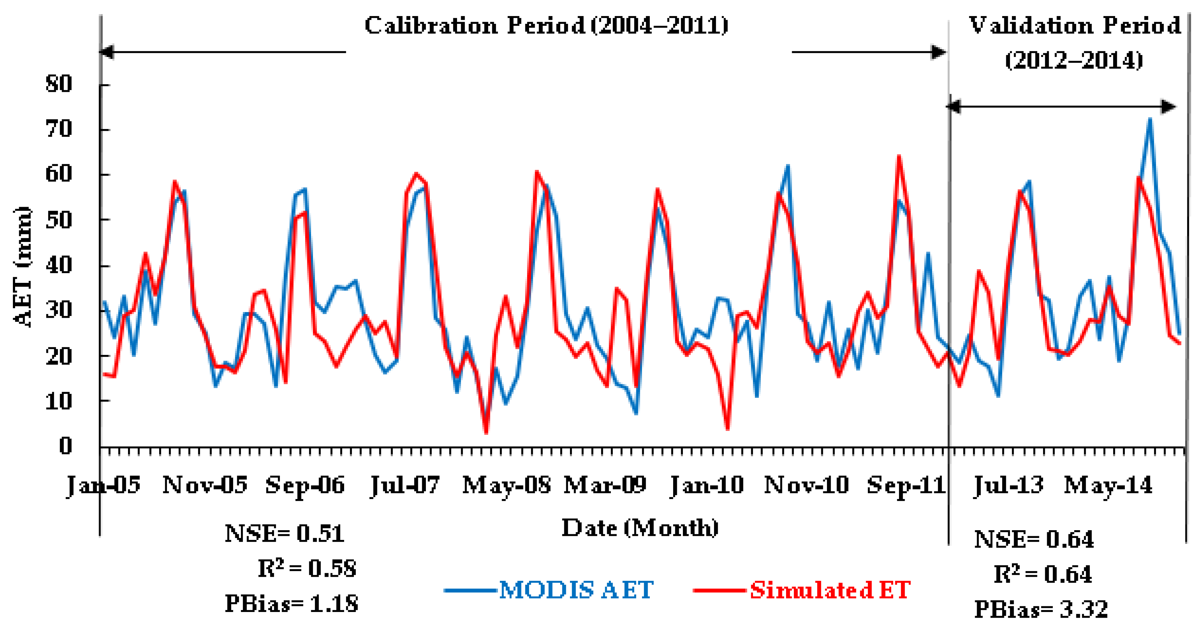
3.2.3. SWAT Model Calibration Using MODIS AET

For the AET-based calibration, the basin has simulated AET performance of NSE (0.64) > 0.5, R2 (0.65) > 0.5, RSR (0.59) ≤ 0.7 with PBias (1.684) ± 25%. For the validation case, the basin has a simulated AET performance of NSE (0.7) > 0.5, R2 (0.73) > 0.5, RSR (0.55) ≤ 0.7 as well as PBias (4.77) < ±25% (Figure 4). These are within the satisfactory ranges proposed by [67,68], whereas, the AET-based simulated streamflow which was evaluated with GloFAS flow at the outlet of the basin has performance values of calibration (NSE (0.45) < 0.5, RSR (0.74) > 0.7 and validation (NSE (0.43) < 0.5 and RSR (0.75 > 0.7) (Figure 5). According to the performance results, employing MODIS AET for calibrating SWAT considerably improves AET simulations over the whole basin, whereas the resultant streamflow simulations at the basin outlet do not meet the required statistical requirements for a satisfactory SWAT model performance [63,64].

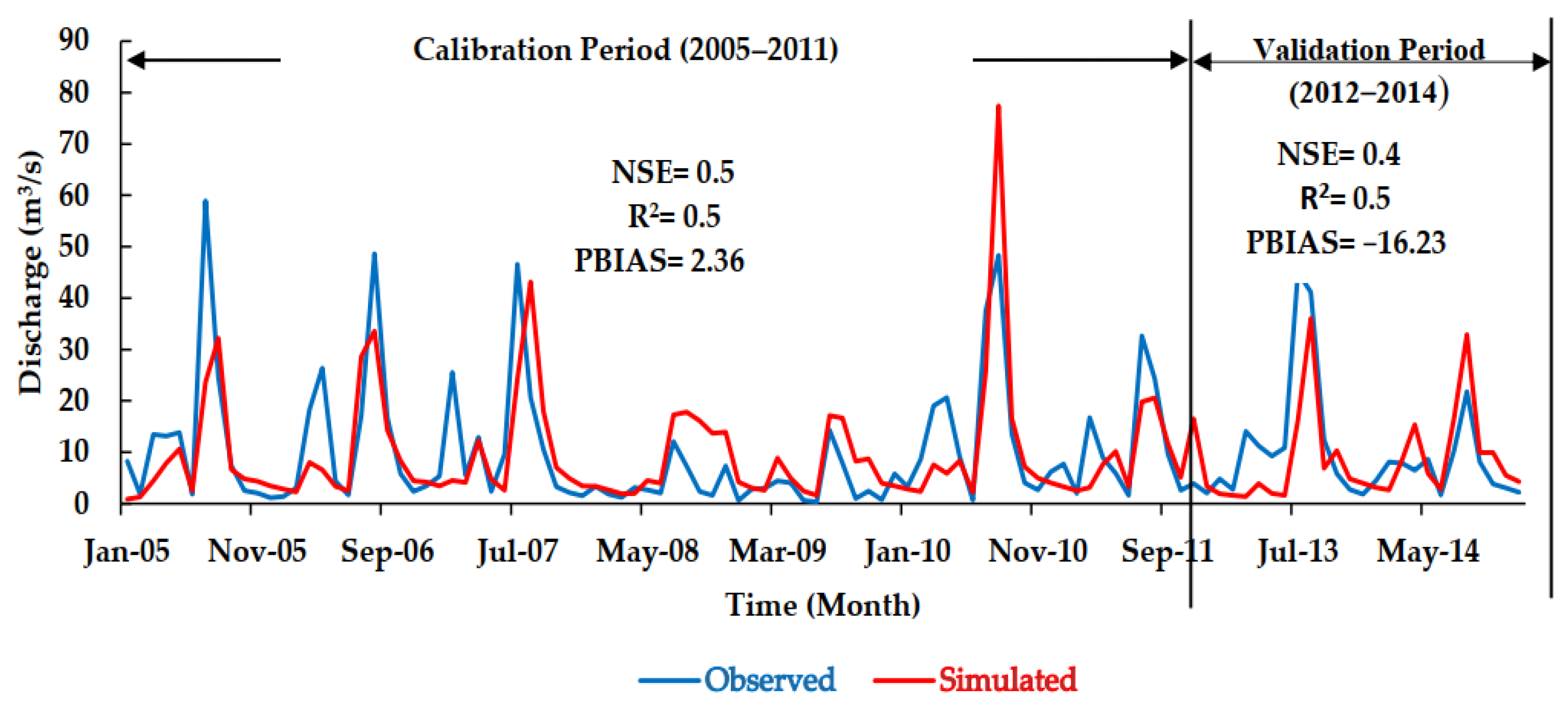
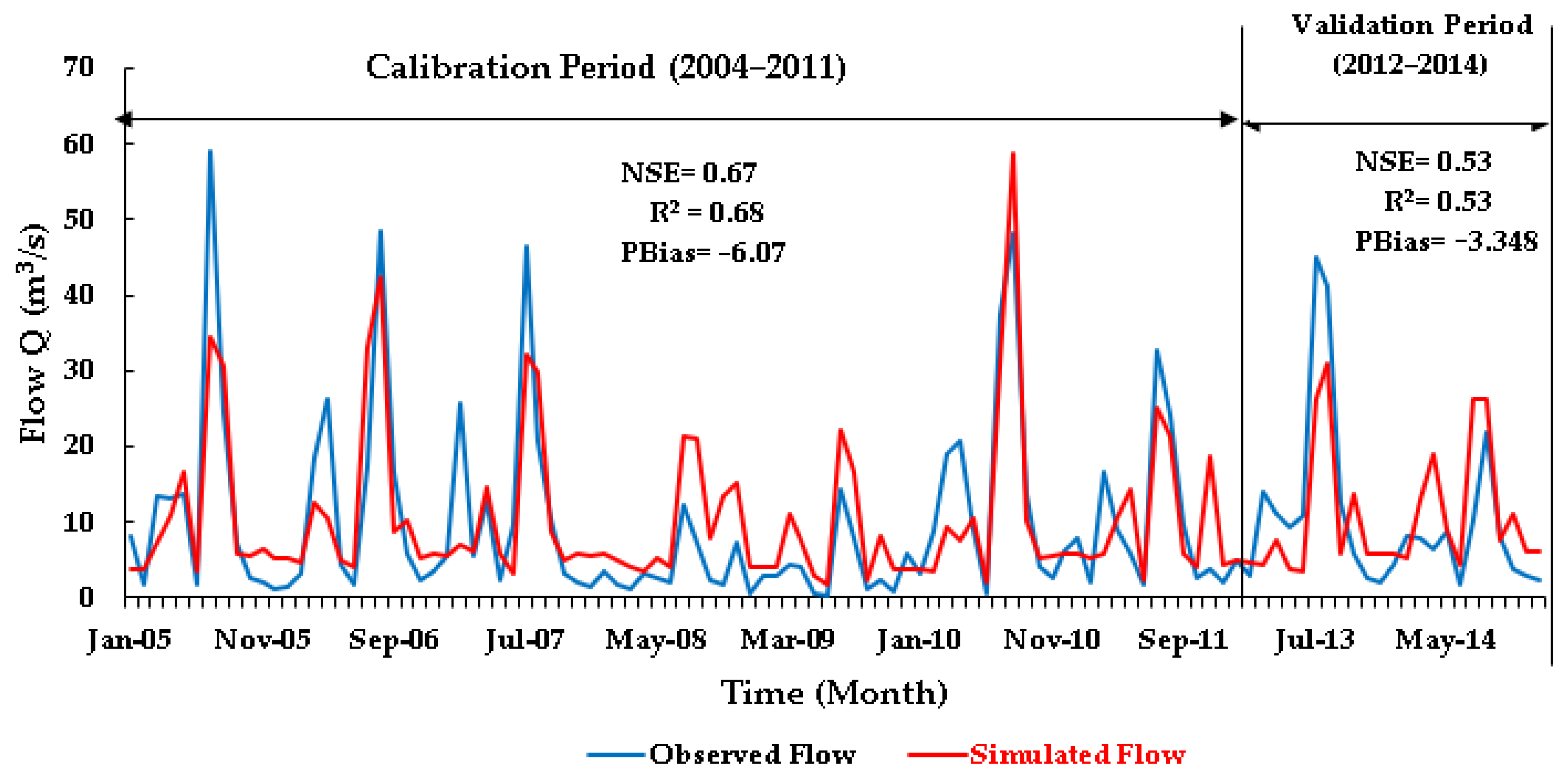
3.2.4. SWAT Model Calibration Using Reanalysis GloFAS River Flow

GloFAS flow was employed for the calibration of the model. Obviously, the simulated output performs better than the uncalibrated SWAT model. For the GloFAS flow-based calibration, the basin has simulated flow performance of NSE (0.67) > 0.5, R2 (0.68) > 0.5, RSR (0.57) ≤ 0.7 with PBias (−6.607) ± 25%. For the validation, the basin has a simulated flow performance of NSE (0.53) > 0.5, R2 (0.53) > 0.5, RSR (0.68) ≤ 0.7, as well as with PBias −3.34 ± 25% (Figure 6).
Simulated AET from GloFAS stream flow-based calibration was also evaluated with MODIS AET at the basin level. In the calibration case, the resulting simulated AET does meet the required statical criteria for a satisfactory SWAT model performance (NSE (0.51), R2 (0.58), > 0.5, RSR (0.7) ≤ 0.7, and PBias 1.185 ± 25%). In the validation case also, the resulting simulated AET at the whole basin does meet the required statical criteria for a satisfactory SWAT model performance (NSE (0.64) > 0.5, R2 (0.64) > 0.5 and RSR (0.60) ≤ 0.7 and PBias (3.327) ± 25% (Figure 7).
The simulated streamflow at the basin outlet and the simulated AET at the basin level meet the statical criteria for satisfactory SWAT model performance during calibration and validation periods [63,64].

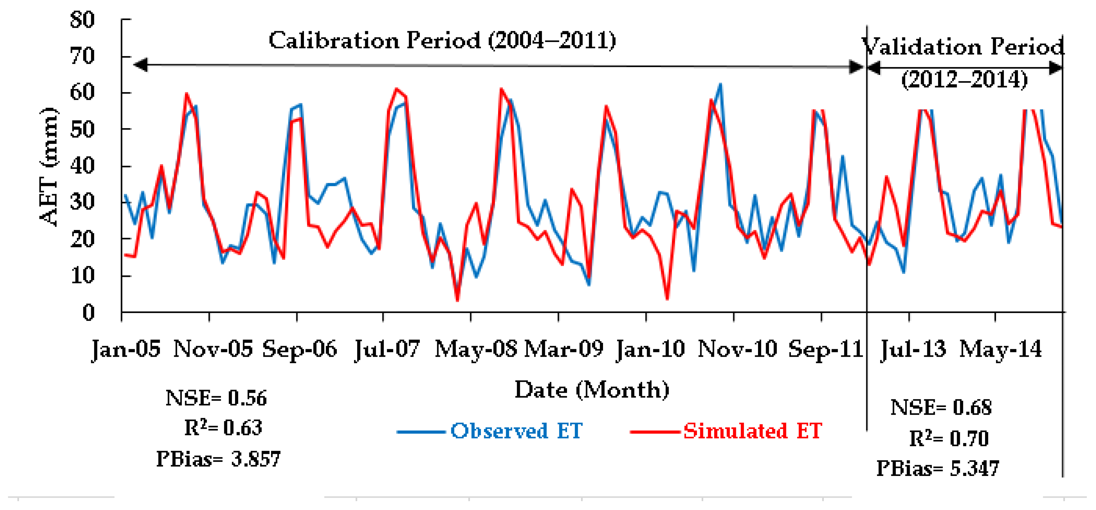
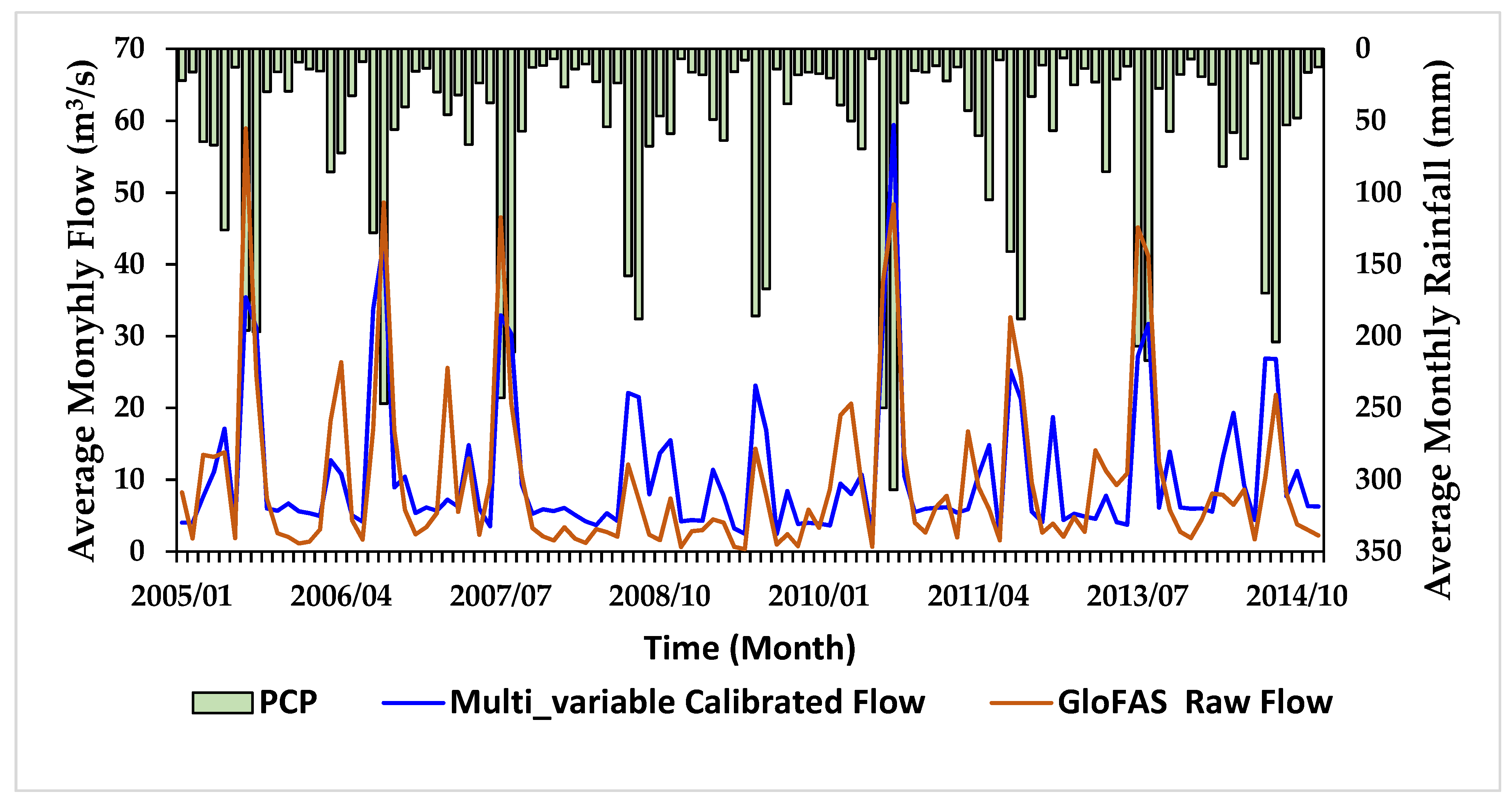
3.2.5. Model Calibration and Validation Using GloFAS River Flow and MODIS AET Concurrently (Multivariable Calibration)

In multi-variable calibration, the basin has simulated flow performance of NSE (0.67) > 0.5, R2 (0.68) > 0.5, RSR (0.57) ≤ 0.7 with PBias (−9.675) ± 25%. For the validation, the basin has a simulated flow performance of NSE (0.54) > 0.5, R2 (0.54) > 0.5, RSR (0.67) ≤ 0.7 as well as with Pbias (−6.221) ± 25%. It is also found that in calibration, the resulting simulated AET does meet the required statical criteria for a satisfactory SWAT model performance (NSE (0.56), R2 (0.58) > 0.5, RSR (0.66) ≤ 0.7 and PBias (3.857) ± 25%). In the validation case also, the resulting simulated AET at the whole basin do meet the required statical criteria for a satisfactory SWAT model performance (NSE (0.68) > 0.5, R2 (0.7) > 0.5 and RSR (0.564) ≤ 0.7 and PBias (5.34) ± 25% (Figure 8 and Figure 9). In both cases, the performance values are within the satisfactory ranges proposed by [63,64]. Table 4 summarizes model calibration and validation efficiencies for all modeling scenarios.
Single and multivariable calibration scenarios attained different model performances for both calibration and validation periods. The single calibration variable, either streamflow or evapotranspiration led to high performance in terms of the calibration/validation variable but impaired performance in the other variable, whereas, the multi-variable calibration scenario reasonably attained the minimum satisfactory performance limit for both variables when compared with the single-variable calibration scenario. Similar studies conducted in Morocco [69], in the Myanmar river basin [68], in the Karkheh river basin of Iran [70], and over the continental USA [71] agreed with the findings of this study that multi-variable calibration performs better than the single variable calibration. Another similar study by [72,73] revealed that multi-variable calibration (evapotranspiration + streamflow) streamflow performance was superior to a single calibration strategy.
Since the multivariable calibration scenario gives reasonable performance for both variables, the parameters are employed to run the model for both the calibration and validation period (2001–2014) at a time to estimate the water balance terms and characterize catchment hydrology.

3.3. Water Balance of the Watershed

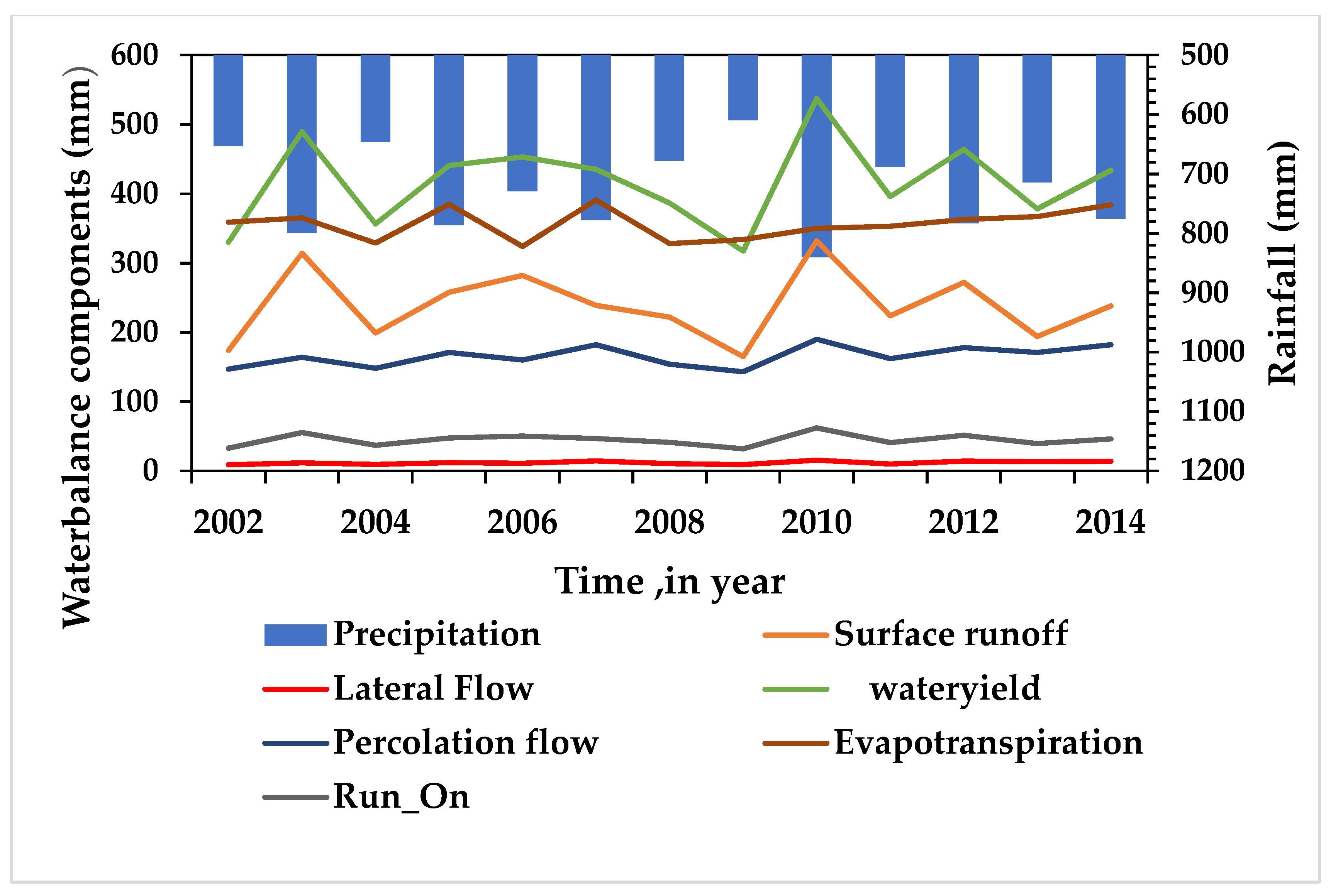
3.3.1. Annual Water Balance Components

To address the problems with water management in the basin, water balance components that are simulated by SWAT+ provide a baseline understanding of the hydrological processes.
The simulated water balance components for each year are presented in Table 5. The annual average precipitation is 729 mm. The percentage of precipitation falling in the dry (October to January), short rainy season (February to June), and the major rainy season (July, August, and September) are 11.9%, 27.64%, and 60.47%, respectively. Similar studies in the Kobo area confirmed that the majority of the rainfall (50%) of the total annual rainfall is derived from the long rain seasons (July, August, and September) in the Kobo area [12].
The surface runoff (SURQ) varied from 165 mm to 332 mm, respectively, with an average annual of 239.46 mm. The minimum and maximum lateral flows were 8.95 mm and 15.6 mm, respectively. The minimum and maximum percolations were also 143 mm and 190 mm, respectively. The minimum and maximum average annual water yields are 317.22 mm and 537.6 mm, respectively. In Table 5, it can be seen that all of the annual water balance components with a higher value are observed during the highest rainy year (2010), whereas, in dry years in which the rainfall is below average (2002, 2004, 2008, 2009, 2011, and 2013), the contribution of water balance components to the water budget decreased significantly. Previous studies in the upper Blue Nile of Ethiopia [74,75] have shown the same trend in that the contribution of water balance components declined with the fall of rainfall.
The year 2002 and 2010 were considered crucial for their minimum and maximum potential of producing water balance components in the catchment, respectively. It is observed that surface runoff, lateral flow, and percolation increase with the increase in rainfall (Figure 10).
The water balance during the simulation period (2002–2014) showed that the catchment receives an annual rainfall of 729 mm. SWAT+ with landscape unit (SWAT + LSU) assumed surface flow -and lateral flow run-on as an additional source of water in the catchment. Therefore the catchment receives 771.63 mm of water annually. Actual evapotranspiration and lateral flow took the major and minor share of the annual water budget, respectively. The actual evapotranspiration, surface runoff, lateral flow, and groundwater recharge (percolation) account for 47%, 30%,1.53%, and 21.4% of the total water in the catchment (precipitation + run-on), respectively.
The result of the water balance assessment showed that 47% of the annual precipitation in the catchment is transferred back to the atmosphere through evapotranspiration. Evapotranspiration holds a major share in the water balance of the catchment. Other previous studies in Ethiopia agree with the findings of this study. A SWAT modeling in the Borkena River Basin showed that evapotranspiration accounts for 48.1% of the total rainfall [76]. A study in the Hormat-Golina River of Ethiopia using the WetSpass model showed that about 68% of precipitation is lost through evapotranspiration [77]. The simulated results from the WEP modeling in the upper Blue Nile of Ethiopia showed that evapotranspiration accounts for a major share (58%) of the total rainfall [74]. In [78], the JGrass-NewAge model system was applied in the upper Blue Nile and found that evapotranspiration accounts for a major share (56%) of the total rainfall. The spatial distribution of water balance components at the HRU level is depicted in Figure 11.

3.3.2. Water Yield and Total Water Storage Assessment

The monthly water balance was also evaluated to see the water yield and storage condition of the catchment. The water yield (WY) accounts for 58.8%, 23.56%, and 17.63% in the main rainy, short rainy, and dry seasons, respectively (Figure 12).
The variation in water yield depends on surface runoff, groundwater, and lateral flow. As a result, water yield followed the same pattern in that it increased with the increase in rainfall. Following the rainfall and runoff pattern, positive storage is obtained (water is stored in soil and ground) for March and April (short rainy season) and July and August (main rainy season).
This is due to the high precipitation and limited evapotranspiration in the rainy seasons, whereas, in the rest of the months (dry season), negative storage was observed, and as a result, water that was stored during the wet seasons is released from the soil and ground to compensate for the deficiency.
Following the precipitation and runoff patterns, maximum positive storage (both in soil and ground) was observed in July (+46.7 mm/month) and August (+26.85 mm/month). Maximum negative storage was observed in September (−53.46 mm/month) and October (−36.36 mm/month). The water stored in the soil during the rainy season will be lost as evapotranspiration in the dry season.

3.4. Surface Runoff Conditions

The spatial pattern of surface runoff follows the rainfall pattern of the catchment. A significant amount of rainfall generated a considerable amount of runoff. The simulated average annual basin surface runoff (SURQ) is 239.46 mm. This shared 30% of the input water of the watershed. The simulated maximum and minimum monthly runoff are attained in August and December with a value of 86.12 mm and 0.67 mm, respectively. Surface runoff generation was found higher in the floodplain areas than in upland areas (Figure 11a). The runoff and rainfall have a direct relationship because of the topography, land cover, and soil infiltration capacity of the catchment. A previous modeling study conducted by [77] around the study area using WetSpass and MODFLOW revealed that the share of surface runoff in the water balance is 27%, which is similar to the findings of the current study.

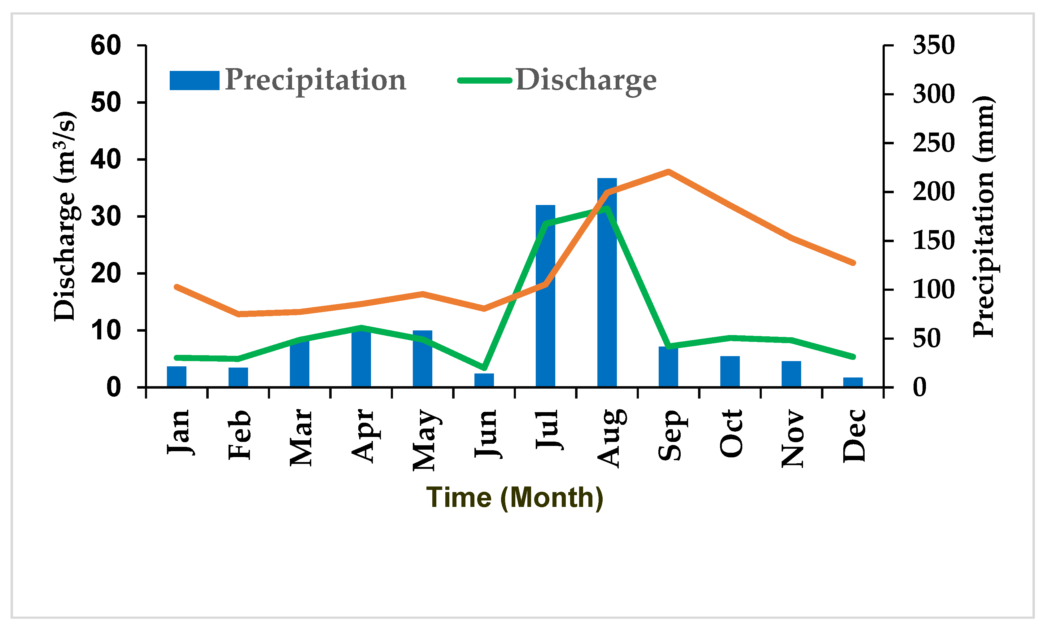
3.5. Streamflow Conditions

Figure 13 showed that the stream flow closely follows the precipitation pattern of the basin. The Mann–Kendall trend test indicated that the daily streamflow showed a significant increasing trend (p < 0.05).
The monthly low flow occurs from October to February and from May to June with a median flow of 1.43 m3/s in June and a coefficient of dispersion of 0.67 and high flows occur in July and August, with a median flow of 16.55 m3/s in August with a coefficient of dispersion of 1.55. The highest coefficient of dispersion (COD) was found in August (the wettest month) and a low coefficient of dispersion was found for the driest month (June) (Table 6).
The simulated minimum and maximum mean annual stream flow at the basin outlet are 7.95 m3/s and 13.2 m3/s (2010), respectively. The maximum flow occurs in the highest rainy year and the lowest flow is observed in the small rainy year (2009). Previous studies showed similar results that in areas where saturation excess runoff dominates, daily discharge is the function of daily rainfall [79,80,81].

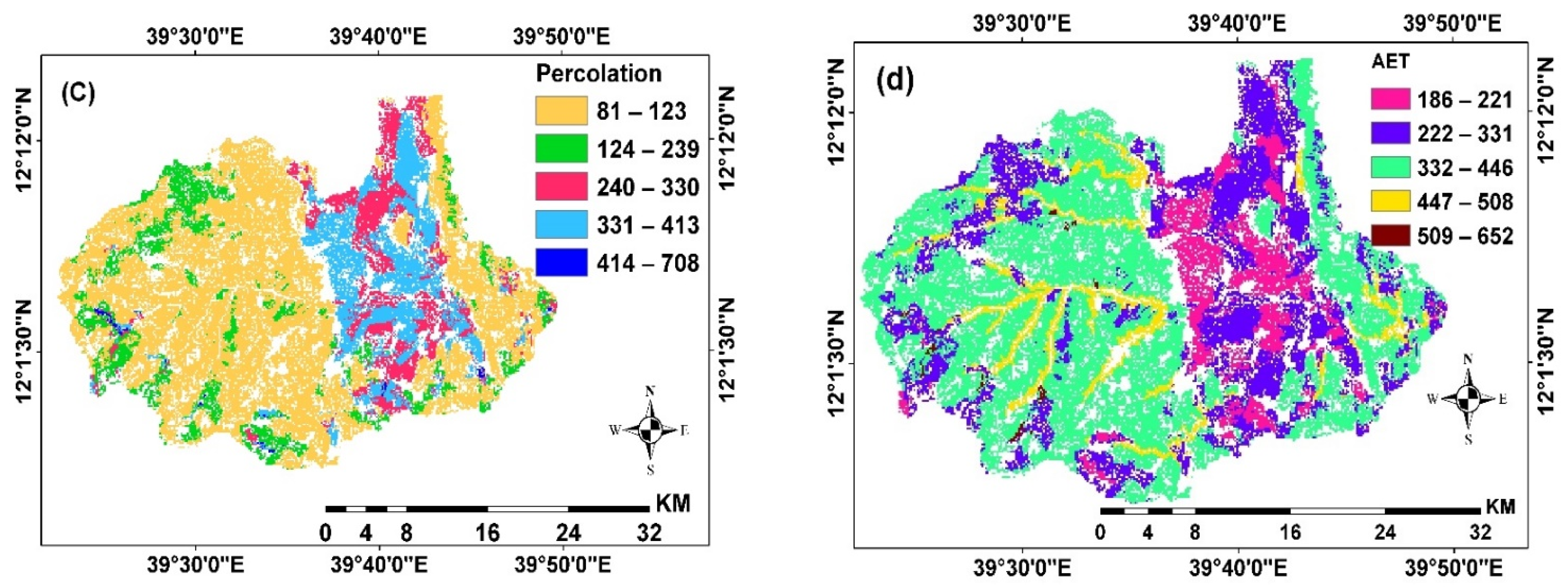
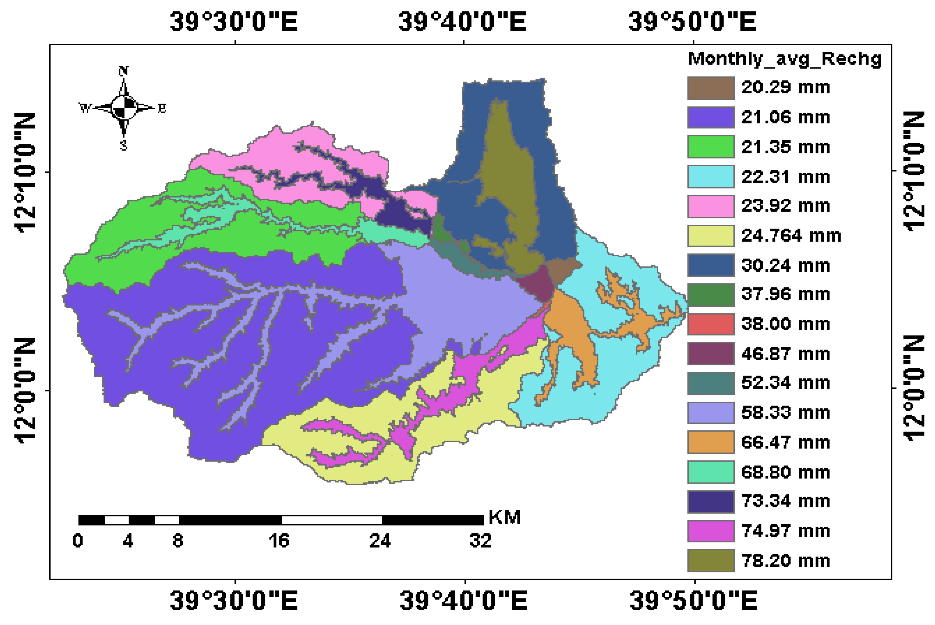
3.6. Recharge Conditions

Groundwater recharge has no real data to prove the performance of the model. Most of the current studies have encountered a similar challenge because of the difficulty in obtaining real data on groundwater recharge. Illuminated by many of the existing studies, we did not directly validate the reliability of groundwater recharge, but validated simulating streamflow instead, assuming that streamflow has a strong correlation to groundwater recharge; this correlation has been substantially represented in the SWAT+ model.
Based on this fact, the simulated model recharge value showed an increasing trend from the upland to the floodplain areas. The minimum and maximum annual recharge are 208 and 276 mm with mean annual recharge of 244.36 mm. The maximum mean monthly simulated recharge is obtained in September (one month later than the month of maximum rainfall) with a value of 78.2 mm (Figure 14). Since the dominant soil in the floodplain area is vertisols, it has a good water-holding capacity and as a result, has a good potential for recharge to the shallow aquifer.
Even if the main rainy season is from June to August, the simulated maximum volume of recharge is observed from September to November. This might be because of the poor capacity of vertisol to release water immediately to the shallow aquifer. This caused a delay in recharge to the aquifer (one month later than the main rainy month). In Figure 14, it is also observed that recharge increases while surface runoff falls from September to December. It can be easily understood that the magnitude of surface runoff is affected by the recharge condition during the storage deficient period.

4. Conclusions

Random utilization of water resources is a threat to the environment. The use of water resources should be based on the recommended exploitable potential. So, understanding the hydrological processes and applying a good hydrological model is the most important aspect of water resource management works. The hydrology of ungauged catchments is still an issue for hydrologists for better management of water resources at different scales. The issue is very critical in developing nations like Ethiopia where there are numerous ungauged catchments. A solution has to be found to tackle the challenge, and hydrological models were considered as one of the means. The SWAT+ model was used to characterize the hydrology of the ungauged catchments of Kobo-Golina.
The water balance terms were properly characterized based on the model simulated result. The study suggested that both surface water harvesting and groundwater exploitation can be sought in floodplain areas while conserving the uplands. It was also found that the use of open-source remote sensing data for model simulation is promising for ungauged areas. CHIRPS reanalysis rainfall can be used as alternative input data for model simulation in the study area. The SWAT+ model simulations also demonstrated that MODIS AET and GloFAS flow present good potential for hydrological model calibration in the study region.
The SWAT+ with LSU (Landscape unit) model setup is very promising with regard to a better representation of hydrological processes in the saturated excess humid areas. This approach paves a new path for characterizing ungauged catchments by SWAT+ hydrological models based on open-source satellite data. The SWAT+ may be used to assess the hydrological processes and quantification of the water balance terms in catchments with similar hydrological and geomorphological features.

Supplementary Materials

The following supporting information can be downloaded at: https://www.mdpi.com/article/10.3390/su15043337/s1, Figure S1. Physical land resources of the study area (A) DEM, (B) Land use, (C) Soil. Figure S2. Landscape of the study area. Table S1: Parameter range and change type to simulated SWAT using MODIS AET and GloFAS river flow.

Author Contributions

Conceptualization, B.Z.A., L.H.; Data curation, B.Z.A.; Formal analysis, B.Z.A., L.H., T.B.T., T.T.A., W.B.A., Funding acquisition, B.Z.A. and L.H.; Investigation, B.Z.A.; Methodology, B.Z.A., L.H., W.B.A., T.T.A.; Project administration, L.H.; Resources, L.H.; Supervision; L.H.; Validation, L.H.; Writing—original draft, B.Z.A.; Writing—review and editing, B.Z.A., L.H., W.B.A., T.B.T., T.T.A. All authors have read and agreed to the published version of the manuscript.

Funding

This research was supported by the National Natural Science Foundation of China (Grant No. 52079088), the Key R&D Program of China (Grant No 2020YFC1807904), and Amhara Design and Supervision Works Enterprise and Tianjin university.

Institutional Review Board Statement

Not applicable.

Informed Consent Statement

Not applicable.

Data Availability Statement

Not applicable.

Acknowledgments

The climate data were obtained from the National Meteorological Agency of Ethiopia. The authors acknowledged financial and technical support from Tianjin University and Amhara Design and Supervision Works Enterprise. The authors acknowledged the three anonymous reviewers who provided comments on the manuscript.

Conflicts of Interest

The authors declare that there is no conflict of interest.

References

  1. Hiwasaki, L. International Decade for Action ‘Water for Life’ 2005–2015. Focus Areas: Water and sustainable development. In Cultural Diversity, and Global Environmental Change; UNESCO: Jakarta, Indonesia, 2011. [Google Scholar]
  2. WBG. Water Resources Management Overview: Development News, Research, Data|World Bank. World Bank Group. 2022. Available online: https://www.worldbank.org/en/topic/waterresourcesmanagement (accessed on 20 December 2022).
  3. Butler, D.; Ward, S.; Sweetapple, C.; Astaraie-Imani, M.; Diao, K.; Farmani, R.; Fu, G. Reliable, resilient and sustainable water management: The Safe & SuRe approach. Glob. Chall. 2017, 1, 63–77. [Google Scholar] [CrossRef] [PubMed]
  4. USAID. Water Resources Profile. 2017. Available online: https://winrock.org/wp-content/uploads/2021/08/Ghana_Country_Profile_Final.pdf (accessed on 20 December 2022).
  5. Adane, Z.; Yohannes, T.; Swedenborg, E.L. Balancing Water Demands and Increasing Climate Resilience: Establishing a Baseline Water Risk Assessment Model in Ethiopia. World Resour. Inst. 2021, 17–18. [Google Scholar] [CrossRef]
  6. WWAP. The United Nations World Water Development Report 2018: Nature-Based Solutions for Water. 2018. Available online: www.unwater.org/publications/%0Aworld-water-development-report-2018/ (accessed on 20 December 2022).
  7. UNICEF. Water Scarcity|UNICEF. Water Scarcity. 2021. Available online: https://www.unicef.org/wash/water-scarcity (accessed on 20 December 2022).
  8. Beyene, M.; Tekle, S.M.; Alemneh, D.G. Open Access Initiatives in Ethiopia’s Higher Learning Institutions. In Handbook of Research on the Global View of Open Access and Scholarly Communications; Alemneh, D.G., Ed.; IGI Global: Hershey, PA, USA, 2022; Available online: https://openresearch.community/documents/pdf-4-1 (accessed on 17 December 2022).
  9. Awulachew, S.B.; Yilma, A.D.; Loulseged, M.; Loiskandl, W.; Ayana, M.; Alamirew, T. Water Resources and Irrigation Development in Ethiopia; Working Paper 123; International Water Management Institute: Colombo, Sri Lanka, 2007; 78p, Available online: https://www.scirp.org/(S(i43dyn45teexjx455qlt3d2q))/reference/referencespapers.aspx?referenceid=1918607 (accessed on 20 October 2022).
  10. Aftab, O. Climate change and water scarcity. In Urban Poverty and Climate Change; Routledge: Oxfordshire, UK, 2018; pp. 167–184. [Google Scholar] [CrossRef]
  11. Adane, Z.; Swedenborg, E.; Yohannes, T. 3 Strategies for Water-Wise Development in Ethiopia. 2021. Available online: https://www.wri.org/insights/strategies-water-risk-insecurity-ethiopia (accessed on 16 December 2022).
  12. Eshetu, Z.; Gebre, H.; Lisanework, N. Impacts of climate change on sorghum production in North Eastern Ethiopia. Afr. J. Environ. Sci. Technol. 2020, 14, 49–63. [Google Scholar] [CrossRef]
  13. Bayable, G.; Amare, G.; Alemu, G.; Gashaw, T. Spatiotemporal variability and trends of rainfall and its association with Pacific Ocean Sea surface temperature in West Harerge Zone, Eastern Ethiopia. Environ. Syst. Res. 2021, 10, 7. [Google Scholar] [CrossRef]
  14. Wondatir, S.; Getnet, A. Determination of supplementary irrigation water requirement and schedule for Sorghum in Kobo-Girana Valley, Ethiopia. Int. J. Agric. Technol. 2021, 17, 385–398. [Google Scholar]
  15. Adane, A. Determinants of adaptation to dry spell in the context of agrarian economy: Insights from Wollo area (Kobo district), Ethiopia. J. Environ. Earth Sci. 2015, 5, 100–115. [Google Scholar]
  16. Adane, G.W. Groundwater Modelling and Optimization of Irrigation Water Use Efficiency to Sustain Irrigation in Kobo Valley, Ethiopia. Master’s Thesis, UNESCO-IHE Institute for Water Education, Delft, The Netherlands, April 2014. [Google Scholar]
  17. Tadesse, N.; Nedaw, D.; Woldearegay, K.; Gebreyohannes, T.; Van Steenbergen, F. Groundwater management for irrigation in the raya and kobo valleys, Northern Ethiopia. Int. J. Earth Sci. Eng. 2015, 8, 1104–1114. [Google Scholar]
  18. Kidane, H. Community Spate Irrigation in Raya Valley: The Case of Three Spate Irrigation Systems; Addis Ababa University: Addis Ababa, Ethiopia, 2009; Available online: http://etd.aau.edu.et/handle/123456789/12122 (accessed on 16 December 2022).
  19. Mengistu, H.A.; Demlie, M.B.; Abiye, T.A. Review: Groundwater resource potential and status of groundwater resource development in Ethiopia. Hydrogeol. J. 2019, 27, 1051–1065. [Google Scholar] [CrossRef]
  20. Abera, K.; Mehari, M. Performance Evaluation of Pressurized Irrigation System (A Case of Kobo Girana Irrigation System, Ethiopia). In Lecture Notes of the Institute for Computer Sciences, Social-Informatics and Telecommunications Engineering, LNICST; Springer: Berlin/Heidelberg, Germany, 2021; Volume 385, pp. 85–97. [Google Scholar] [CrossRef]
  21. Nedaw, D.; Tafesse, N.T.; Woldearegay, K.; Gebreyohannes, T.; Van Steenbergen, F.; Willibald, L. Groundwater Based Irrigation and Food Security in Raya-Kobo Valley, Northern Ethiopia. Asian Rev. Environ. Earth Sci. 2018, 5, 15–21. [Google Scholar] [CrossRef]
  22. Chow, V.T.; Maidment, D.R.; Mays, L.W.; Chow, L.W.M.V.T.; Maidment, D.R. Applied Hydrology Chow; McGraw-Hill: New York, NY, USA, 1998; pp. 1–294. Available online: http://ponce.sdsu.edu/Applied_Hydrology_Chow_1988.pdf (accessed on 15 October 2022).
  23. Gupta, A.; Himanshu, S.K.; Gupta, S.; Singh, R. Evaluation of the SWAT Model for Analysing the Water Balance Components for the Upper Sabarmati Basin. In Lecture Notes in Civil Engineering; Springer: Singapore, 2020; Volume 39, pp. 141–151. [Google Scholar] [CrossRef]
  24. Abbaspour, K.C.; Rouholahnejad, E.; Vaghefi, S.; Srinivasan, R.; Yang, H.; Kløve, B. A continental-scale hydrology and water quality model for Europe: Calibration and uncertainty of a high-resolution large-scale SWAT model. J. Hydrol. 2015, 524, 733–752. [Google Scholar] [CrossRef]
  25. Akoko, G.; Le, T.; Gomi, T.; Kato, T. A review of swat model application in africa. Water 2021, 13, 1313. [Google Scholar] [CrossRef]
  26. Dile, Y.T.; Srinivasan, R. Evaluation of CFSR climate data for hydrologic prediction in data-scarce watersheds: An application in the blue nile river basin. J. Am. Water Resour. Assoc. 2014, 50, 1226–1241. [Google Scholar] [CrossRef]
  27. Duan, Z.; Tuo, Y.; Liu, J.; Gao, H.; Song, X.; Zhang, Z.; Yang, L.; Mekonnen, D.F. Hydrological evaluation of open-access precipitation and air temperature datasets using SWAT in a poorly gauged basin in Ethiopia. J. Hydrol. 2019, 569, 612–626. [Google Scholar] [CrossRef]
  28. Bekele, D.; Alamirew, T.; Kebede, A.; Zeleke, G.; Melesse, A.M. Modeling Climate Change Impact on the Hydrology of Keleta Watershed in the Awash River Basin, Ethiopia. Environ. Model. Assess. 2019, 24, 95–107. [Google Scholar] [CrossRef]
  29. Fentaw, F.; Hailu, D.; Nigussie, A.; Melesse, A.M. Climate Change Impact on the Hydrology of Tekeze Basin, Ethiopia: Projection of Rainfall-Runoff for Future Water Resources Planning. Water Conserv. Sci. Eng. 2018, 3, 267–278. [Google Scholar] [CrossRef]
  30. Hailu, M.B. Identifying and prioritizing Sediment-prone areas at the sub-basin level of Tekeze watershed, Ethiopia. Res. Sq. 2022, PPR524327. [Google Scholar] [CrossRef]
  31. Steenhuis, T.S.; Schneiderman, E.M.; Mukundan, R.; Hoang, L.; Moges, M.; Owens, E.M. Revisiting SWAT as a saturation-excess runoff model. Water 2019, 11, 1427. [Google Scholar] [CrossRef]
  32. Bieger, K.; Arnold, J.G.; Rathjens, H.; White, M.J.; Bosch, D.D.; Allen, P.M.; Volk, M.; Srinivasan, R. Introduction to SWAT+, A Completely Restructured Version of the Soil and Water Assessment Tool. J. Am. Water Resour. Assoc. 2017, 53, 115–130. [Google Scholar] [CrossRef]
  33. Odusanya, A.E.; Schulz, K.; Biao, E.I.; Degan, B.A.; Mehdi-Schulz, B. Evaluating the performance of streamflow simulated by an eco-hydrological model calibrated and validated with global land surface actual evapotranspiration from remote sensing at a catchment scale in West Africa. J. Hydrol. Reg. Stud. 2021, 37, 100893. [Google Scholar] [CrossRef]
  34. Bennour, A.; Jia, L.; Menenti, M.; Zheng, C.; Zeng, Y.; Barnieh, B.A.; Jiang, M. Calibration and Validation of SWAT Model by Using Hydrological Remote Sensing Observables in the Lake Chad Basin. Remote Sens. 2022, 14, 1511. [Google Scholar] [CrossRef]
  35. Wedajo, G.K.; Muleta, M.K.; Awoke, B.G. Performance evaluation of multiple satellite rainfall products for Dhidhessa River Basin (DRB), Ethiopia. Atmos. Meas. Tech. 2021, 14, 2299–2316. [Google Scholar] [CrossRef]
  36. Mengistu, A.G.; Woldesenbet, T.A.; Dile, Y.T. Evaluation of observed and satellite-based climate products for hydrological simulation in data-scarce Baro -Akob River Basin, Ethiopia. Ecohydrol. Hydrobiol. 2022, 22, 234–245. [Google Scholar] [CrossRef]
  37. Bennett, N.D.; Croke, B.F.W.; Guariso, G.; Guillaume, J.H.A.; Hamilton, S.H.; Jakeman, A.J.; Marsili-Libell, S.; Newham, L.T.H.; Norton, J.P.; Perrin, C.; et al. Characterising performance of environmental models. Environ. Model. Softw. 2013, 40, 1–20. [Google Scholar] [CrossRef]
  38. Kessete, N.; Moges, M.A.; Steenhuis, T.S. Evaluating the applicability and scalability of bias corrected CFSR climate data for hydrological modeling in upper Blue Nile basin, Ethiopia. Extrem. Hydrol. Clim. Var. 2019, 2019, 11–22. [Google Scholar]
  39. Rajib, A.; Evenson, G.R.; Golden, H.E.; Lane, C.R. Hydrologic model predictability improves with spatially explicit calibration using remotely sensed evapotranspiration and biophysical parameters. J. Hydrol. 2018, 567, 668–683. [Google Scholar] [CrossRef]
  40. Ha, L.T.; Bastiaanssen, W.G.M.; van Griensven, A.; van Dijk, A.I.J.M.; Senay, G.B. Calibration of spatially distributed hydrological processes and model parameters in SWAT using remote sensing data and an auto-calibration procedure: A case study in a Vietnamese river basin. Water 2018, 10, 212. [Google Scholar] [CrossRef]
  41. Karra, K.; Kontgis, C.; Statman-Weil, Z.; Mazzariello, J.C.; Mathis, M.; Brumby, S.P. Global land use/land cover with Sentinel 2 and deep learning. In Proceedings of the 2021 IEEE International Geoscience and Remote Sensing Symposium IGARSS, Brussels, Belgium, 11–16 July 2021; IEEE: Piscataway, NJ, USA, 2021; pp. 4704–4707. [Google Scholar] [CrossRef]
  42. Hengl, T.; Heuvelink, G.B.M.; Kempen, B.; Leenaars, J.G.B.; Walsh, M.G.; Shepherd, K.D.; Sila, A.; Macmillan, R.A.; De Jesus, J.M.; Tamene, L.; et al. Mapping soil properties of Africa at 250 m resolution: Random forests significantly improve current predictions. PLoS ONE 2015, 10, e0125814. [Google Scholar] [CrossRef]
  43. Harrigan, S.; Zsoter, E.; Alfieri, L.; Prudhomme, C.; Salamon, P.; Wetterhall, F.; Barnard, C.; Cloke, H.; Pappenberger, F. GloFAS-ERA5 operational global river discharge reanalysis 1979–present. Earth Syst. Sci. Data 2020, 12, 2043–2060. [Google Scholar] [CrossRef]
  44. Senent-aparicio, J.; Blanco-gómez, P.; López-ballesteros, A.; Jimeno-sáez, P.; Pérez-sánchez, J. Evaluating the potential of glofas-era5 river discharge reanalysis data for calibrating the swat model in the grande san miguel river basin (El salvador). Remote Sens. 2021, 13, 3299. [Google Scholar] [CrossRef]
  45. Beven, K.; Freer, J. Equifinality, data assimilation, and uncertainty estimation in mechanistic modelling of complex environmental systems using the GLUE methodology. J. Hydrol. 2001, 249, 11–29. [Google Scholar] [CrossRef]
  46. Favis-Mortlock, D. Self-Organization and Cellular. In Environmental Modelling: Finding Simplicity in Complexity; Wiley Blackwell: New York, NY, USA, 2004; p. 349. [Google Scholar]
  47. Beven, K. Rainfall-Runoff Modelling; John Wiley & Sons: Hoboken, NJ, USA, 2012. [Google Scholar] [CrossRef]
  48. Bitew, M.M.; Gebremichael, M. Evaluation of satellite rainfall products through hydrologic simulation in a fully distributed hydrologic model. Water Resour. Res. 2011, 47, W06526. [Google Scholar] [CrossRef]
  49. Shah, S.; Duan, Z.; Song, X.; Li, R.; Mao, H.; Liu, J.; Ma, T.; Wang, M. Evaluating the added value of multi-variable calibration of SWAT with remotely sensed evapotranspiration data for improving hydrological modeling. J. Hydrol. 2021, 603, 127046. [Google Scholar] [CrossRef]
  50. Abiodun, O.O.; Guan, H.; Post, V.E.A.; Batelaan, O. Comparison of MODIS and SWAT evapotranspiration over a complex terrain at different spatial scales. Hydrol. Earth Syst. Sci. 2018, 22, 2775–2794. [Google Scholar] [CrossRef]
  51. Herman, M.R.; Nejadhashemi, A.P.; Abouali, M.; Hernandez-Suarez, J.S.; Daneshvar, F.; Zhang, Z.; Anderson, M.C.; Sadeghi, A.M.; Hain, C.R.; Sharifi, A. Evaluating the role of evapotranspiration remote sensing data in improving hydrological modeling predictability. J. Hydrol. 2018, 556, 39–49. [Google Scholar] [CrossRef]
  52. Kunnath-Poovakka, A.; Ryu, D.; Renzullo, L.J.; George, B. The efficacy of calibrating hydrologic model using remotely sensed evapotranspiration and soil moisture for streamflow prediction. J. Hydrol. 2016, 535, 509–524. [Google Scholar] [CrossRef]
  53. Immerzeel, W.; Droogers, P. Calibration of a distributed hydrological model based on satellite evapotranspiration. J. Hydrol. 2008, 349, 411–424. [Google Scholar] [CrossRef]
  54. Dile, Y.T.; Ayana, E.K.; Worqlul, A.W.; Xie, H.; Srinivasan, R.; Lefore, N.; You, L.; Clarke, N. Evaluating satellite-based evapotranspiration estimates for hydrological applications in data-scarce regions: A case in Ethiopia. Sci. Total Environ. 2020, 743, 140702. [Google Scholar] [CrossRef] [PubMed]
  55. Mu, Q.; Zhao, M.; Running, S.W. Improvements to a MODIS global terrestrial evapotranspiration algorithm. Remote Sens. Environ. 2011, 115, 1781–1800. [Google Scholar] [CrossRef]
  56. Monteith, J.L. Reply. Q. J. R. Meteorol. Soc. 1964, 90, 107. [Google Scholar] [CrossRef]
  57. SWAT+ Toolbox - Home. Available online: https://celray.github.io/docs/swatplus-toolbox/v1.0/index.html (accessed on 22 October 2022).
  58. Nash, J.E.; Sutcliffe, J. River flow forecasting through conceptual models part I—A discussion of principles. J. Hydrol. 1970, 10, 282–290. [Google Scholar] [CrossRef]
  59. Perez-Valdivia, C.; Cade-Menun, B.; McMartin, D.W. Hydrological modeling of the pipestone creek watershed using the Soil Water Assessment Tool (SWAT): Assessing impacts of wetland drainage on hydrology. J. Hydrol. Reg. Stud. 2017, 14, 109–129. [Google Scholar] [CrossRef]
  60. Yen, H.; Wang, X.; Fontane, D.G.; Harmel, R.D.; Arabi, M. A framework for propagation of uncertainty contributed by parameterization, input data, model structure, and calibration/validation data in watershed modeling. Environ. Model. Softw. 2014, 54, 211–221. [Google Scholar] [CrossRef]
  61. Saltelli, A.; Ratto, M.; Andres, T.; Campolongo, F.; Cariboni, J.; Gatelli, D.; Saisana, M.; Tarantola, S. Sensitivity Analysis: From Theory to Practice; John Wiley & Sons: Hoboken, NJ, USA, 2008. [Google Scholar] [CrossRef]
  62. Onyutha, C. Statistical Uncertainty in Hydrometeorological Trend Analyses. Adv. Meteorol. 2016, 2016, 8701617. [Google Scholar] [CrossRef]
  63. Moriasi, D.N.; Arnold, J.G.; Van Liew, M.W.; Bingner, R.L.; Harmel, R.D.; Veith, T.L. Model evaluation guidelines for systematic quantification of accuracy in watershed simulations. Trans. ASABE 2007, 50, 885–900. [Google Scholar] [CrossRef]
  64. Kouchi, D.H.; Esmaili, K.; Faridhosseini, A.; Sanaeinejad, S.H.; Khalili, D.; Abbaspour, K.C. Sensitivity of calibrated parameters and water resource estimates on different objective functions and optimization algorithms. Water 2017, 9, 384. [Google Scholar] [CrossRef]
  65. Wassie, S.B.; Mengistu, D.A.; Berlie, A.B. Trends and spatiotemporal patterns of meteorological drought incidence in North Wollo, northeastern highlands of Ethiopia. Arab. J. Geosci. 2022, 15, 1158. [Google Scholar] [CrossRef]
  66. Hordofa, A.T.; Leta, O.T.; Alamirew, T.; Kawo, N.S.; Chukalla, A.D. Performance evaluation and comparison of satellite-derived rainfall datasets over the Ziway lake basin, Ethiopia. Climate 2021, 9, 113. [Google Scholar] [CrossRef]
  67. Reda, K.W.; Liu, X.; Haile, G.G.; Sun, S.; Tang, Q. Hydrological evaluation of satellite and reanalysis-based rainfall estimates over the Upper Tekeze Basin, Ethiopia. Hydrol. Res. 2022, 53, 584–604. [Google Scholar] [CrossRef]
  68. Sirisena, T.A.J.G.; Maskey, S.; Ranasinghe, R. Hydrological model calibration with streamflow and remote sensing based evapotranspiration data in a data poor basin. Remote Sens. 2020, 12, 3768. [Google Scholar] [CrossRef]
  69. López, P.L.; Sutanudjaja, E.H.; Schellekens, J.; Sterk, G.; Bierkens, M.F.P. Calibration of a large-scale hydrological model using satellite-based soil moisture and evapotranspiration products. Hydrol. Earth Syst. Sci. 2017, 21, 3125–3144. [Google Scholar] [CrossRef]
  70. Rientjes, T.H.M.; Muthuwatta, L.P.; Bos, M.G.; Booij, M.J.; Bhatti, H.A. Multi-variable calibration of a semi-distributed hydrological model using streamflow data and satellite-based evapotranspiration. J. Hydrol. 2013, 505, 276–290. [Google Scholar] [CrossRef]
  71. Ferguson, C.R.; Sheffield, J.; Wood, E.F.; Gao, H. Quantifying uncertainty in a remote sensing-based estimate of evapotranspiration over continental USA. Int. J. Remote Sens. 2010, 31, 3821–3865. [Google Scholar] [CrossRef]
  72. Franco, A.C.L.; Bonumá, N.B. Multi-variable SWAT model calibration with remotely sensed evapotranspiration and observed flow. RBRH 2017, 22, 011716090. [Google Scholar] [CrossRef]
  73. Koltsida, E.; Kallioras, A. Multi-Variable SWAT Model Calibration Using Satellite-Based Evapotranspiration Data and Streamflow. Hydrology 2022, 9, 112. [Google Scholar] [CrossRef]
  74. Abebe, S.A.; Qin, T.; Zhang, X.; Li, C.; Yan, D. Estimating the Water Budget of the Upper Blue Nile River Basin with Water and Energy Processes (WEP) Model. Front. Earth Sci. 2022, 10, 923252. [Google Scholar] [CrossRef]
  75. Leta, M.K.; Demissie, T.A.; Tränckner, J. Modeling and prediction of land use land cover change dynamics based on land change modeler (Lcm) in nashe watershed, upper blue nile basin, Ethiopia. Sustainability 2021, 13, 3740. [Google Scholar] [CrossRef]
  76. Yesuf, H.M.; Melesse, A.M.; Zeleke, G.; Alamirew, T. Streamflow prediction uncertainty analysis and verification of SWAT model in a tropical watershed. Environ. Earth Sci. 2016, 75, 806. [Google Scholar] [CrossRef]
  77. Bezabih, S.; Alemayehu, T. “Groundwater Recharge Assessment Using WetSpass and MODFLOW Coupling: The Case of Hormat-Golina Sub-basin, Northern Ethiopia. Am. J. Water Sci. Eng. 2022, 8, 7. [Google Scholar] [CrossRef]
  78. Abera, W.; Formetta, G.; Brocca, L.; Rigon, R. Modeling the water budget of the Upper Blue Nile basin using the JGrass-NewAge model system and satellite data. Hydrol. Earth Syst. Sci. 2017, 21, 3145–3165. [Google Scholar] [CrossRef]
  79. Enku, T.; Melesse, A.M.; Ayana, E.K.; Tilahun, S.A.; Abate, M.; Steenhuis, T.S. Groundwater use of a small Eucalyptus patch during the dry monsoon phase. Biologia 2020, 75, 853–864. [Google Scholar] [CrossRef]
  80. Abebe, W.B.; Tilahun, S.A.; Moges, M.M.; Wondie, A.; Derseh, M.G.; Nigatu, T.A.; Mhiret, D.A.; Steenhuis, T.S.; Van Camp, M.; Walraevens, K.; et al. Hydrological foundation as a basis for a holistic environmental flow assessment of tropical highland rivers in ethiopia. Water 2020, 12, 547. [Google Scholar] [CrossRef]
  81. Li, M.; Di, Z.; Duan, Q. Effect of sensitivity analysis on parameter optimization: Case study based on streamflow simulations using the SWAT model in China. J. Hydrol. 2021, 603, 126896. [Google Scholar] [CrossRef]
Figure 1. Location of the study area.
Sustainability 15 03337 g001
Figure 2. Scatter plot and correlation coefficient determination of rain gauge station and CHIRPS rainfall data.
Sustainability 15 03337 g002
Figure 3. Scatter plot and correlation coefficient determination of measured streamflow and GloFAS flow data at the upper Golina weir site.
Sustainability 15 03337 g003
Figure 4. MODIS AET and simulated AET based on MODIS AET calibration.
Sustainability 15 03337 g004
Figure 5. GloFAS and simulated hydrograph based on MODIS AET calibration.
Sustainability 15 03337 g005
Figure 6. GloFAS and simulated hydrographs based on GloFAS flow calibration.
Sustainability 15 03337 g006
Figure 7. MODIS AET and simulated AET based on GloFAS flow calibration.
Sustainability 15 03337 g007
Figure 8. MODIS AET and simulated AET based on Calibration of multiple variables.
Sustainability 15 03337 g008
Figure 9. GloFAS flow and simulated hydrographs based on Calibration of multiple variables.
Sustainability 15 03337 g009
Figure 10. Distribution of mean annual value of simulated water balance components (2002–2014).
Sustainability 15 03337 g010
Figure 11. Spatial distribution of average annual water balance components at HRU level. (a) Surface runoff generated (b) Lateral flow (c) Percolation, and (d) Actual evapotranspiration.
Sustainability 15 03337 g011aSustainability 15 03337 g011b
Figure 12. Mean monthly simulated (2002–2014) water balance Kobo-Golina (Long time simulated value based on parameters from multivariable calibration).
Sustainability 15 03337 g012
Figure 13. A rainfall-runoff pattern of the Kobo-Golina sub-basin at the main outlet (2002–2014).
Sustainability 15 03337 g013
Figure 14. Average monthly recharge for September.
Sustainability 15 03337 g014
Table 2. Landscape/Land use/Soil/Slope and HRU distribution in the basin.
Id No Area [ha]% Watershed
1Watershed104,092.2
2Landscape units
Floodplain30,021.3928.84
Upslope74,070.8171.16
3Land use
URML (Urban Medium Density)2331.552.24
AGRL (Agricultural land generic)70,584.967.81
FRST (Forest)6319.86.07
RNGB (Range Shrubland)23,834.7422.9
South Western Range +Bed rock (SWRN)80.610.08
PAST (Pasture land)633.430.61
WETW (Water)307.170.3
4Soil
LP (Leptosols)73,768.4670.87
CM (CambiSols)5973.075.74
VR (VertiSols)23,983.1323.04
LV (LuviSols)367.540.35
5Slope
0–5.018,590.417.86
5.0–8.07269.696.98
8.0–15.010,796.8110.37
15.0–30.018,645.8117.91
30.0–999948,789.4946.87
Table 3. Sensitivity analysis of calibrated parameters with their optimal values and rank.
SWAT ParameterDescriptionGloFAS Flow-Based CalibrationMODIS AET- Based CalibrationGloFAS Flow and MODIS ET
Based Calibration
1st-Order Sensitivity ValueRank1st-Order Sensitivity ValueRank1st-Order Sensitivity ValueRank
r_ cn2.hruSCS Curve Number0.7410210.1081930.96151
v_ esco.hruSoil evaporation compensation factor−0.00200680.0333350.013675
a_ canmx.hruMaximum canopy storage0.000NS0.000NS0.000NS
r_bd.sol (mg/ cm3)Moist bulk density0.0000260.000NS0.000NS
r_ bd.sol (g/m3)Moist bulk density0.0027950.002287−0.00846
v_ alpha.aquBase flow alpha factor−0.00636100.000NS−0.01757
a_ k.solSaturated hydraulic conductivity−0.0234190.0109360.02434
v_ epco.hruPlant uptake compensation factor0.0617830.209322−0.031189
a_ awc.solAvailable water capacity of the soil layer0.1453120.5916410.19502
v_ perco.hruPercolation coefficient0.0432140.0488640.05613
v_ revap_min.aquThreshold depth of water in the shallow aquifer for “revap” or percolation to the deep aquifer to occur0.000NS0.000NS0.000NS
r_cn3_ swf.hruPothole evaporation coefficient−0.000570.000878−0.024268
v_ flo_min.aquMinimum aquifer storage to allow return flow−0.13588110.00NS−0.0595310
NS: Not sensitive, “v_” represents a replacement (existing parameter value is to be replaced by a given value); “r_” represents a relative change (existing parameter value is multiplied by 1+ given value within the range); “a_” represents the given value is added to the existing parameter values. The parameter with the most sensitive values is shown in bold type. Sensitivity rank is indicated by the values in brackets.
Table 4. Model calibration and validation efficiencies for all scenarios.
Model ScenarioVariablePerformance Evaluation for the Calibration Period (2004–2011)Performance Evaluation for the Validation Period (2012–2014)
DefaultGloFAS river flowNSE 0.06
R2 0.48
PBias 30.09
RSR 0.96
NSE 0.21
R2 0.59
PBias 31.10
RSR 0.88
MODIS AETNSE −1.68
R2 0.23
PBias −39.66
RSR 1.63
NSE −0.38
R2 0.31
PBias −30.03
RSR 1.17
Calibration/validation based on GloFAS flow onlyComparison between raw GloFAS flow and simulated flow dataNSE 0.67
R2 0.68
PBias −6.607
RSR 0.572
NSE 0.54
R2 0.54
PBias −3.348
RSR 0.68
Comparison between raw MODIS AET and simulated AET dataNSE 0.51
R2 0.58
PBias 1.18
RSR 0.7
NSE 0.64
R2 0.64
PBias 3.32
RSR 0.60
Calibration/validation based on MODIS AET onlyComparison between raw MODIS AET and simulated AET dataNSE 0.64
R2 0.65
PBias 1.68
RSR 0.599
NSE 0.69
R2 0.73
PBias 4.77
RSR 0.554
Comparison between raw GloFAS flow and simulated flow dataNSE 0.5
R2 0.5
PBias 2.36
RSR 0.74
NSE 0.4
R2 0.5
PBias −16.23
RSR 0.752
Calibration/validation based on both GloFAS and MODIS AETComparison between raw GloFAS flow and simulated flow dataNSE 0.67
R2 0.68
PBias −9.675
RSR 0.57
NSE 0.54
R2 0.54
PBias −6.22
RSR 0.67
Comparison between raw MODIS AET and simulated AET dataNSE 0.56
R2 0.63
PBias 3.857
RSR 0.66
NSE 0.68
R2 0.70
PBias 5.347
RSR 0.56
Table 5. Mean annual Water Balance components of Kobo-Golina catchment (2002–2014).
YearAnnual Input Water (PCP + Run On)SURQLATQPerc.Water YieldAETRun_OnSum of Water Balance Components
2002685.751748.95147329.9535932.75688.95
2003854.2931411.7164489.736555.29854.7
2004682.851999.36148356.3632936.85685.36
2005833.72581217144138547.7826
2006779.3928211.2160453.232450.39777.2
2007824.623914.3182435.339146.6826.3
2008719.2522210.6154386.632841.25714.6
2009641.871659.22143317.2233431.87651.22
2010902.133215.6190537.635062.1887.6
2011728.8222410.1162396.135340.82749.1
2012834.427214.1178464.136351.4827.1
2013753.519413.2171378.236739.5745.2
2014821.123813.9182433.938446.1817.9
Annual average773.9723911.86165.5416.8356.344.8773.17
Table 6. Monthly median flows (m3/s) of Kobo-Golina at the outlet (2002–2014). Q25 is the flow that is exceeded 25% of the time, Q50 is the median, and Q75 is the flow that exceeded 75% of the time.
MonthMedian Flow (Q50)Coefficient of Dispersions (Q75 − Q25)/Q50)MonthMedian Flow (Q50)Coefficient of Dispersions (Q75 − Q25)/Q50)
Jan2.9181.028Jul15.131.59
Feb2.1520.96Aug16.551.55
Mar5.8751.01Sep6.3341.21
Apr8.9141.22Oct2.5270.88
May2.1091.18Nov1.7670.59
Jun1.430.67Dec1.6911.1
Disclaimer/Publisher’s Note: The statements, opinions and data contained in all publications are solely those of the individual author(s) and contributor(s) and not of MDPI and/or the editor(s). MDPI and/or the editor(s) disclaim responsibility for any injury to people or property resulting from any ideas, methods, instructions or products referred to in the content.

