Influence of Clean Energy and Financial Structure on China’s Provincial Carbon Emission Efficiency—Empirical Analysis Based on Spatial Spillover Effects

Abstract

Clean energy is an essential means to limiting carbon emissions and improving economic transformation, and a market-oriented financial structure is the inevitable result of the deepening of supply-side financial reforms. Exploring whether clean energy enhances carbon emission efficiency (CEE) through financial structural adjustment is essential in formulating policies intended to achieve the dual goals of “carbon peaking” and “carbon neutrality”. As part of the evaluation of China’s provincial CEE using panel data of 30 provinces from 2000 to 2019, this paper adopts an improved nonradial directional distance function (NDDF), while empirically analyzing the influence of clean energy and a market-oriented financial structure on CEE using a spatial econometric model. The results indicate the following findings: (1) The provincial CEE in China is characterized by significant spatial autocorrelation. (2) A 1% increase in the integration of clean energy and a market-oriented financial structure leads to a 0.0032% increase in the local CEE and a 0.0076% increase in neighboring regions’ CEE through the spatial spillover effect. Clean energy can efficiently enhance CEE through the stock market, while it has a passive impact through bank credit. (3) The interactive effect between clean energy and a market-oriented financial structure varies according to the provincial CEE. From the 25th to the 90th quantiles, the role of clean energy in promoting CEE through the capital market is very significant, while clean energy inhibits CEE through bank credit in most provinces. Therefore, China’s clean energy development will bolster its competitiveness in the global market through a market-oriented financial structure that will bring economic development and environmental pollution into balance and provide a theoretical foundation for China’s double carbon reduction.

1. Introduction

Climate warming has a profound influence on the continued survival of human beings and has thus become a priority in the global community. At present, China is already the world’s largest carbon dioxide (CO₂) emitter. As an accountable country, China has committed to reducing carbon emissions as outlined at the Copenhagen Conference, as well as to the dual carbon emission goals (i.e., achieving carbon peak by 2030 and carbon neutrality by 2060) at the General Assembly of the United Nations. China is therefore under tremendous pressure to reduce its CO₂ emissions. China has emerged as the world’s second-largest economy and has enjoyed moderate to high economic growth since the country’s reform and opening up over the last 40 years. However, China’s past economic growth was the result of industrial production that required excessive energy consumption and created excessive pollution and emissions, which urgently requires the transformation to high-quality economic development. Lowering CO₂ emissions is fundamental for China’s sustainable development, but the government should also continue to develop the economy and raise living conditions [1]. It has therefore become an urgent issue for both scholars and policymakers to achieve the dual carbon goals while maintaining steady economic development. For the developing countries that are represented by China, enhancing carbon emission efficiency (CEE) is an advantageous way to meet this demand [2], while coordinating CO₂ emissions with economic activity [3].

Energy is the backbone of manufacturing and people’s living standards and thus drives socioeconomic improvement [4]. However, traditional fossil fuels create welfare while producing a massive amount of CO₂ emissions [5,6]. Given the concern for global warming, most scholars view clean energy as a vital alternative to fossil energy [7,8,9]. It is therefore beneficial to explore the relationship between clean energy development and CEE to support decision making for promoting sustainable economic growth and limiting CO₂ emissions [10]. Meanwhile, a stable financial system also has a crucial role to play in economic and environmental terms. From the perspective of structural transformation, different stages of economic growth will face various environmental issues; then there are also structural differences in the financial system’s response to environmental problems. Some studies have shown that the market-oriented financial structure has an important impact on economic development and carbon emission reduction [11,12]. Theoretically, the change of financial structure also plays a crucial role in CEE. As China’s structural supply-side financial reforms continue to deepen, it may facilitate the flow of capital to clean industries and mitigate environmental pollution [13]. However, bank credit tends to be less good at financing clean energy, while capital market is more conducive to clean energy development [14]. As such, whether the integration of clean energy development and financial structure transformation can become a key way to enhance CEE, so as to achieve carbon emission reduction targets and long-term economic development, is of critical value to both China and the world.

At present, the research on CEE is focused on the following two aspects: On the one hand, it is about the definition and calculation of CEE. The early definition of CEE involved single-factor indicators, and its ease of use has received significant interest from academics. Other scholars have adopted other indicators to define carbon emission performance [15,16]. Despite this, the one-factor approach can only capture a small portion of carbon efficiency and fails to reveal the importance of other factors that affect CEE (such as labor force, capital accumulation, and energy inputs) [17]. It is for this reason that total factor indicators, which include more than one input and output involved in the production process, have attracted a great deal of attention [17]. Generally, total factor performance indicators have been calculated using the frontier approach, which measures performance as the distance between the inputs and outputs and the production frontier. There are two methods to measure performance: stochastic frontier analysis (SFA) and data envelopment analysis (DEA). SFA is a parametric method that requires a predetermined production function and is exceedingly subjective, which may lead to deviations in the calculating results [18]. However, DEA is a nonparametric method that does not need to assume a function form or random component distribution, and is suitable for evaluating performance through multi-input/output indicators. Accordingly, some researchers incorporate CO₂ into the undesirable output and obtain CEE through slack-based measure (SBM), directional distance function (DDF), and nonradial directional distance function (NDDF) [19,20,21,22]. It should be noted that the technological heterogeneity among regions [20] and the inconsistency between desirable and undesirable outputs [23] are not considered in the efficiency calculation, which will lead to some deviations and errors in the results.

On the other hand, enhancing CEE has also been explored. Some researchers have produced promising results in terms of industrial structure [24], green technology [22], urbanization, and foreign direct investment [25]. However, as an effective way to limit CO₂ emissions and achieve the sustainable development goals [26], the influence of clean energy on CEE has been broadly ignored. Previous studies have focused more on the impact of clean (or renewable) energy on economic growth and CO₂ emissions, but have not yet reached a consensus [27,28,29]. Meanwhile, as China’s financial system continues to improve, it has shifted from a single banking system to a multilevel financial market system. Whether structural financial reforms should contribute to economic growth and promote energy conservation and emission reduction cannot be ignored. Some researchers have also begun to examine the role of financial structure in reducing carbon emissions [11,12]. In addition, compared with the bank-led financial structure, the capital market is more conducive to promoting clean energy development [30,31]. However, there is little literature that provides in-depth analysis of clean energy and financial structure as an effective way to enhance CEE.

Considering that China is a large country with regional heterogeneity, regional differences are apparent in CEE due to its economic development, industrial distribution, energy endowment, environmental pollution, and other factors [21,22]. Clean energy development is inconsistent across regions [32], and there is also variability in the extent to which market-oriented financial structures affect each region [33]. Therefore, clean energy development and financial structure transformation may have different impacts and extents across different regions when it comes to carbon efficiency. The aim of this article is therefore to further elaborate on our discussion by applying a spatial econometric model.

In view of the gap in the existing literature, this paper aims to analyze the influence of clean energy and financial restructuring on provincial CEE in China. Specifically, the principal contributions of this study are as follows: First, this study applies the improved NDDF to calculate the CEE at the provincial level in China. We find that there is a sizeable spatial imbalance, which provides a basis for policy makers to recognize the current status of CEE and take robust measures. Second, unlike previous studies, we put clean energy, financial structure, and CEE into a single framework. Third, we systematically explore the influence of clean energy and a market-oriented financial structure on CEE and include the spillover effects. Meanwhile, we classify Chinese provinces into groups according to their CEE level to explore the variability in the influence of regional clean energy under different financing channels. This method provides a theoretical foundation for enhancing CEE in each region in China and formulating financial support mechanisms for clean energy in a localized manner.

Following is a description of the rest of this study. Review of the literature is provided in Section 2. The hypotheses of the study are presented in Section 3. The data and methods of research are described in Section 4. An analysis and presentation of the empirical results are provided in Section 5. A discussion of policy implications concludes Section 6.

2. Literature Review

2.1. The Influence of Clean Energy on Economic Growth and Carbon Emissions

Clean energy development is considered a vital way to rebalance economic growth and improve environmental quality. However, it is a double-edged sword in that its economic benefits remain controversial. It was argued by Salim et al. [27] that renewable energy was an alternative to fossil fuels that could stimulate the economy. The study of Inglesi-Lotz [34] focused on the economic growth of OECD countries and found that renewable energy consumption had a positive effect on growth. Based on studying the 10 countries with the highest CO₂ emissions, Azam et al. [28] found that expanding and improving renewable and nuclear energy supplies could result in the economic growth and reduction of greenhouse gas emissions. In addition, some research has discovered that renewable energy could stimulate economic growth through mechanisms such as boosting employment and increasing per capita income [35]. It has been demonstrated that developing (or non-OECD) countries can only increase their economic growth when their renewable energy consumption meets a certain threshold based on the scale effect [36]. However, initial fixed costs are high for clean energy development, usually borne by the government at the beginning [37]. Subsidies for clean energy not only distort the energy market but also have a crowding-out effect on other government expenditures [10]. Thus, clean energy development may also dampen economic growth.

In fact, some studies have disputed the emission reduction benefits of clean energy. From the perspective of the substitution effect, clean energy replaces traditional fossil energy and optimizes the energy mix, which is beneficial to CO₂ emissions reduction [7,8,29]. However, it has also been found that the technology and rebound effects of clean energy have a potentially negative impact on CO₂ emissions. For instance, Qi et al. [38] found that renewable energy storage technology was still immature, while it could not meet peak load demand, so suppliers had to use fossil energy, which offset the substitution effect from renewables. Based on their research, Balsalobre-Lorente et al. [5] concluded that generating renewable energy stimulates economic growth while increasing fossil fuel consumption, which in turn contributes to greenhouse gas emissions. Based on spatial effects, Chen et al. [9] documented that clean energy had a small impact on local CO₂ emissions, but a large impact on CO₂ emissions in neighboring regions. Furthermore, some scholars argue that renewable energy does not contribute to carbon emission reduction until a critical threshold is reached [39]. In the context of declining subsidies, capital markets play an increasingly important role in clean energy’s role in reducing carbon emissions [14].

2.2. The Influence of Financial Structure on Economic Growth and Carbon Emissions

It cannot be ignored that structural financial reforms can contribute to economic growth while also increasing energy efficiency and reducing emissions. In the existing studies, the roles of banks and financial markets in promoting economic growth are treated differently. On the one hand, a major advantage of banks is that they are capable of allocating resources, managing risks, and providing credit, which promotes economic growth and alleviates concerns with external financing [40,41]. On the other hand, firms can obtain significant capital and information from the market to improve their operations, which enhances economic growth to some extent [42,43]. Due to the variety of financing services provided by banks and financial markets, differentiated financial structures have become more crucial to economic growth, especially in the current phase of economic transformation and upgrading [44,45].

Previous studies have focused on financial development, and with the increasing importance of financial structure, scholars have begun to emphasize its role in carbon emission reduction [11,46]. However, there are inconsistent views on the impact of market-oriented financial structures on CO₂ emissions. By taking traditional manufacturing industries with high levels of energy consumption and pollution as an example, Matemilola et al. [47] found that firms from these industries were generally highly leveraged, and when they experienced difficulty in obtaining loans from banks, they raised funds from the stock market by making a public offering. Increasing the proportion of direct financing will inevitably increase energy consumption and drive up CO₂ emissions. Other studies identify the disincentive effect, where the market-oriented financial structure is more conducive to technological innovation than the bank-led financial structure [48], which implies that the former may form an innovative emission reduction mechanism. In the environmentally friendly companies that have gone public, Yao and Tang [46] found that financing ratios were negatively related to CO₂ emissions.

3. Research Hypothesis

Carbon emission efficiency is an important evaluation indicator of low carbon economy, that is, an effective basis for reconciling economic growth with carbon emission reduction [10]. Theoretically, the factor and substitution effects of clean energy can effectively promote economic development and reduce CO₂ emissions, which implies that clean energy has great potential to enhance CEE. However, this potential has been greatly diminished by the lack of mature technologies and the large capital requirements needed in the early developmental stages. With the gradual removal of government subsidies further constraining clean energy development, external financing has become an inevitable choice for companies. Unlike the risk-averse nature of the banking industry, the stock market favors high-risk, high-return projects such as clean energy [30], and is therefore willing to provide direct financing opportunities for concepts such as clean energy [14]. Additionally, the capital market can mitigate the adverse selection and moral hazard issues to a large extent. Clean energy companies have increased in valuation because of investor demand for social responsibility and more informative disclosure requirements [49], which has provided reliable sources of financing for the clean energy industry. As capital funds gradually flow to the green sector, it will alleviate the difficulty of financing the clean energy industry, thus unleashing the potential of clean energy in enhancing CEE. Therefore, we propose our first hypothesis.

H1. 

The integration of clean energy and stock market can improve CEE.

Currently, the banking industry remains the most important component of China’s financial system. Functionally, banks are more sophisticated than capital markets in terms of capital reserves, information management, and risk control, so they can play a more important role in promoting economic growth [14]. Despite China undergoing a period of economic transition, there is significant credit discrimination in financial institutions, particularly in state-owned commercial banks [50]. As a result of this, commercial banks are more likely to provide credit to state-owned or listed companies, which limits access to financial services and loans for green firms. In addition, the banking industry is risk-averse, and its loan review processes are not only very strict but also time-consuming [11]. For example, Nasir et al. [51], in studying ASEAN economies, found that the banking industry provides more credit channels for energy-intensive sectors, while green industries obtain very little. In turn, this phenomenon is causing the clean energy industry and its related technology R&D projects to have difficulty obtaining sufficient funding from commercial banks, which may adversely affect CEE. On the basis of the above analysis, we propose the second hypothesis.

H2. 

The combination of clean energy and the banking industry may reduce CEE.

Existing studies have shown that if one region produces and consumes energy, it is likely to affect the production and consumption of energy in adjoining regions and vice versa [52]. Clean energy is mainly supplied and consumed in the form of electricity, and the impact between regions is particularly evident [9]. Chica-Olmo et al. [53], for example, found that stimulated renewable energy consumption promoted both domestic economic growth and the economic growth of neighboring countries, thus showing the spatial spillover effects of renewable energy use. Compared with banking institutions, which are restricted by business premises, financial markets have stronger liquidity and wider distribution characteristics and can therefore improve the cross-regional allocation of financial resources, reduce transaction costs and mitigate information asymmetries, and provide a favorable financing environment for clean energy enterprises in neighboring regions. As clean energy is incorporated more widely in neighboring regions, economic growth is promoted, and carbon emissions are reduced, which improves the quality of the environment. Therefore, we propose our third hypotheses.

H3: 

The neighboring CEE can be enhanced through a spatial spillover effect, which combines clean energy with a market-oriented financial structure.

4. Methodology and Data

4.1. Evaluation of Carbon Emission Efficiency

In this study, the CEE at the provincial level in China is evaluated using the DEA method based on its definition of environment production technology function. It is the provinces that are considered decision-making units (DMUs). Each DMU takes capital stock, labor force, and energy consumption as input variables to produce gross domestic product (GDP), which then generates carbon dioxide emissions. It is also necessary to ensure that the production set is compatible with the weak disposability and null jointness assumptions [54], and the extent to which CO₂ emissions are reduced should be measured by GDP, since GDP alone can serve as a means of eliminating CO₂. Therefore, the production technology set (P) is constructed as follows:

$$P=\{(K,L,E,Y,C):(K,L,E) can produce (Y,C)\}$$

(1)

where K means capital stock, L indicates the labor force, E implies energy consumption, Y is actual GDP as desirable output, and C represents CO₂ emissions as undesirable output.

Due to differences in the levels of socioeconomic development among provinces in China, the technological heterogeneity among regions is high [20]. As a result, when all regions are included in a single production frontier, there can be no accurate representation of technological differences between them. Considering the technology gaps between different DMUs [55,56], this paper divides all DMUs into h groups, with each h containing N^h DMUs and satisfying ${\displaystyle {\sum }_{h=1}^H{N}^h}=N$ [21]. The inputs and outputs of all DMUs in each group are taken into the same P. Suppose that $P_h^C$ is defined as the contemporaneous frontier, thus denoting that all observations are contained in group h during the period. The intertemporal frontier of group h can be defined as $P_h^I=\left\{P_h^1\cup P_h^2\cdots P_h^T\right\}$, which contains all observations of all periods of group h. The global frontier can be defined as $P^G=\left\{P_{h1}^I\cup P_{h2}^I\cdots P_H^I\right\}$, which contains all observations of all group h’s in all periods.

Environmental performance is usually evaluated by distance function. To calculate efficiency, Chambers et al. [57] developed a directional distance function (DDF). Fukuyama and Weber [58] pointed out that this radical measure overestimates efficacy in situations of slack. In order to overcome the problem of equal proportional variation of inputs and outputs in DDF, Zhou et al. [19] proposed NDDF as follows:

$$\overrightarrow{ND}=(K,L,E,Y,C;g)=sup\left\{{\omega }^T\beta :((K,L,E,Y,C)+g\times diag(\beta ))\in P\right\}$$

(2)

where ${\omega }^T={({\omega }_K,{\omega }_L,{\omega }_E,{\omega }_Y,{\omega }_C)}^T$ denotes the weight vector of input variables, desirable output and undesirable output; $g=(-g_K,-g_L,-g_E,g_Y,-g_C)$ represents a directional vector; $\beta ={({\beta }_K,{\beta }_L,{\beta }_E,{\beta }_Y,{\beta }_C)}^T\ge 0$ indicates a scale factor vector that measures the inefficiency of inputs and outputs; and $diag(\beta )$ is the diagonal matrix where the diagonal element equals $\beta$.

Zhang and Choi [59] argue that input and output variables should be given equal weight due to DEA not having a specific functional form. Therefore, following Zhang and Liu [60], we select ${\omega }^T={(0,0,\frac{1}{3},\frac{1}{3},\frac{1}{3})}^T$ and define the directional vector as $g=(0,0,-E,Y,-C)$.

Following Cheng et al. [23] and Zhang and Liu [60], the optimal ${\beta }^{*C}$ of the contemporaneous frontier can be obtained using linear programming and by excluding the influence of K and L.

$$\begin{array}{l}{\overrightarrow{ND}}^C(K,L,E,Y,C;g^C)=\max \{\frac{1}{3}{\beta }_E^C+\frac{1}{3}{\beta }_Y^C+\frac{1}{3}{\beta }_C^C\}\\ s.t.{\displaystyle \sum _{n=1}^{N^h}{\lambda }_n^t{K}_n^t}\le K,{\displaystyle \sum _{n=1}^{N^h}{\lambda }_n^t{L}_n^t}\le L,{\displaystyle \sum _{n=1}^{N^h}{\lambda }_n^t{E}_n^t}\le (1-{\beta }_E^C)E,\\ {\displaystyle \sum _{n=1}^{N^h}{\lambda }_n^t{Y}_n^t}\ge (1+{\beta }_Y^C)Y,{\displaystyle \sum _{n=1}^{N^h}{\lambda }_n^t{C}_n^t}=(1-{\beta }_C^C)C\\ {\lambda }_n^t\ge 0, {\beta }_Y^C\ge 0, 0\le {\beta }_K^C,{\beta }_L^C,{\beta }_E^C,{\beta }_C^C\le 1,\\ n=1,2,\cdots ,N^h\end{array}$$

(3)

Furthermore, the optimal ${\beta }^{*I}$ of the group intertemporal frontier can be obtained by solving Equation (4).

$$\begin{array}{l}{\overrightarrow{ND}}^I(K,L,E,Y,C;g^I)=\max \{\frac{1}{3}{\beta }_E^I+\frac{1}{3}{\beta }_Y^I+\frac{1}{3}{\beta }_C^I\}\\ s.t.{\displaystyle \sum _{t=1}^T{\displaystyle \sum _{n=1}^{N^h}{\lambda }_n^t{K}_n^t}}\le K,{\displaystyle \sum _{t=1}^T{\displaystyle \sum _{n=1}^{N^h}{\lambda }_n^t{L}_n^t}}\le L\\ {\displaystyle \sum _{t=1}^T{\displaystyle \sum _{n=1}^{N^h}{\lambda }_n^t{E}_n^t}}\le (1-{\beta }_E^I)(1-{\beta }_E^C)E\\ {\displaystyle \sum _{t=1}^T{\displaystyle \sum _{n=1}^{N^h}{\lambda }_n^t{Y}_n^t}}\ge (1+{\beta }_Y^I)(1+{\beta }_Y^C)Y\\ {\displaystyle \sum _{t=1}^T{\displaystyle \sum _{n=1}^{N^h}{\lambda }_n^t{C}_n^t}}=(1-{\beta }_C^I)(1-{\beta }_C^C)C\\ {\lambda }_n^t\ge 0, {\beta }_Y^I\ge 0, 0\le {\beta }_K^I,{\beta }_L^I,{\beta }_E^I,{\beta }_C^I\le 1,\\ t=1,2,\cdots ,T,n=1,2,\cdots ,N^h\end{array}$$

(4)

Finally, the optimal ${\beta }^{*G}$ of the global frontier of NDDF can be obtained by solving Equation (5).

$$\begin{array}{l}{\overrightarrow{ND}}^G(K,L,E,Y,C;g^G)=\max \{\frac{1}{3}{\beta }_E^G+\frac{1}{3}{\beta }_Y^G+\frac{1}{3}{\beta }_C^G\}\\ s.t.{\displaystyle \sum _{h=1}^H{\displaystyle \sum _{t=1}^T{\displaystyle \sum _{n=1}^{N^h}{\lambda }_n^t{K}_n^t}}}\le K,{\displaystyle \sum _{h=1}^H{\displaystyle \sum _{t=1}^T{\displaystyle \sum _{n=1}^{N^h}{\lambda }_n^t{L}_n^t}}}\le L\\ {\displaystyle \sum _{h=1}^H{\displaystyle \sum _{t=1}^T{\displaystyle \sum _{n=1}^{N^h}{\lambda }_n^t{E}_n^t}}}\le (1-{\beta }_E^G)(1-{\beta }_E^I)(1-{\beta }_E^C)E\\ {\displaystyle \sum _{h=1}^H{\displaystyle \sum _{t=1}^T{\displaystyle \sum _{n=1}^{N^h}{\lambda }_n^t{Y}_n^t}}}\ge (1+{\beta }_Y^G)(1+{\beta }_Y^I)(1+{\beta }_Y^C)Y\\ {\displaystyle \sum _{h=1}^H{\displaystyle \sum _{t=1}^T{\displaystyle \sum _{n=1}^{N^h}{\lambda }_n^t{C}_n^t}}}=(1-{\beta }_C^G)(1-{\beta }_C^I)(1-{\beta }_C^C)C\\ {\lambda }_n^t\ge 0, {\beta }_Y^G\ge 0, 0\le {\beta }_K^G,{\beta }_L^G,{\beta }_E^G,{\beta }_C^G\le 1,\\ t=1,2,\cdots ,T,n=1,2,\cdots ,N^h,h=1,2,\cdots ,H\end{array}$$

(5)

Based on the optimal solution obtained above, following Zhang and Liu [60], the CEE can be formulated as:

$$CE{E}_{it}=\frac{1/2[(1-{\beta }_{E,it}^{*G})(1-{\beta }_{E,it}^{*I})(1-{\beta }_{E,it}^{*C})]+1/2[(1-{\beta }_{C,it}^{*G})(1-{\beta }_{C,it}^{*I})(1-{\beta }_{C,it}^{*C})]}{(1+{\beta }_{Y,it}^{*G})(1+{\beta }_{Y,it}^{*I})(1+{\beta }_{Y,it}^{*C})}$$

(6)

It is clear that CEE ranges from 0 to 1, and the greater the score is, the better the CEE is.

4.2. Methodology and Data

This paper first constructs the benchmark model following this format to test clean energy’s impact on CEE:

$$CE{E}_{it}={\alpha }_0+{\alpha }_1{X}_{it}+{\displaystyle \sum _k{\alpha }_k}Control{s}_{k,it}+{\mu }_i+{\lambda }_t+{\epsilon }_{it}$$

(7)

In Equation (7), i and t represent the province and year, respectively. CEE is the explained variable; X is the core explanatory variable, which contains clean energy (CE) and the financial structure (FS). As part of the Controls, we refer to the variables related to government intervention (GOV), industrial structure (IS), energy structure (ES), trade openness (TO), and environmental regulation (ER). ${\mu }_i$, ${\lambda }_t$, and ${\epsilon }_{it}$ denote individual fixed effects, time fixed effects, and the random error term, respectively. In past studies, clean energy [9], financial development [61], and CEE [22] are all variables with significant spatial geographic characteristics, and ignoring these spatial correlations may result in biased empirical results. To avoid this bias, we incorporate spatial variables into the above benchmark model. It has been proposed that spatial econometric models can be divided into spatial lag models (SLM), spatial error models (SEM), and spatial Durbin models (SDM) based on the research framework presented by Elhorst et al. [62]. Compared with SLM and SEM, SDM can effectively estimate the influence of local and neighboring independent variables on dependent variables and thus reflect spatial effects between regions [63]. Therefore, this paper constructs SDM as follows:

$$\begin{array}{ll}CE{E}_{it}=& \rho WCE{E}_{it}+{\beta }_{1}lnC{E}_{it}+{\beta }_{2}F{S}_{it}+{\displaystyle \sum _k{\beta }_{k}Control{s}_{k,it}}\\ & +{\theta }_{1}WlnC{E}_{it}+{\theta }_{2}WF{S}_{it}+{\displaystyle \sum _k{\theta }_{k}WControl{s}_{it}}+{\mu }_i+{\lambda }_t+{\epsilon }_{it}\end{array}$$

(8)

$$\begin{array}{ll}CE{E}_{it}=& \rho WCE{E}_{it}+{\beta }_{1}lnC{E}_{it}+{\beta }_{2}STOC{K}_{it}+{\displaystyle \sum _k{\beta }_{k}Control{s}_{k,it}}\\ & +{\theta }_{1}WlnC{E}_{it}+{\theta }_{2}WSTOC{K}_{it}+{\displaystyle \sum _k{\theta }_{k}WControl{s}_{it}}+{\mu }_i+{\lambda }_t+{\epsilon }_{it}\end{array}$$

(9)

$$\begin{array}{ll}CE{E}_{it}=& \rho WCE{E}_{it}+{\beta }_{1}lnC{E}_{it}+{\beta }_{2}BAN{K}_{it}+{\displaystyle \sum _k{\beta }_{k}Control{s}_{k,it}}\\ & +{\theta }_{1}WlnC{E}_{it}+{\theta }_{2}WBAN{K}_{it}+{\displaystyle \sum _k{\theta }_{k}WControl{s}_{it}}+{\mu }_i+{\lambda }_t+{\epsilon }_{it}\end{array}$$

(10)

In Equations (8)–(10), FS is the proportion of total stock market transactions in bank loans and thus indicates the financial structure; STOCK is the proportion of total stock market transactions in GDP, thus representing the financial market; and BANK is the ratio of bank loans to GDP, which represents the banking industry. Spatial regression coefficient $\rho$ indicates the strength of the spatial spillover effect, while spatial lag variables ${\theta }_i (i=1,2,\cdots )$ indicate how neighboring variables affect the variables that are explained. ln indicates that the variables take the natural logarithm form.

Furthermore, to investigate the effect of combining clean energy and financial structure on CEE, the interaction term of clean energy and the financial structure is introduced into Equations (8)–(10). The resulting models are as follows:

$$\begin{array}{ll}CE{E}_{it}=& \rho WCE{E}_{it}+{\beta }_{1}lnC{E}_{it}+{\beta }_{2}F{S}_{it}+{\beta }_{3}lnC{E}_{it}*F{S}_{it}+{\displaystyle \sum _k{\beta }_{k}Control{s}_{it}}\\ & +{\theta }_{1}WlnC{E}_{it}+{\theta }_{2}WF{S}_{it}+{\theta }_{3}WlnC{E}_{it}*F{S}_{it}+{\displaystyle \sum _k{\theta }_{k}WControl{s}_{it}}+{\mu }_i+{\lambda }_t+{\epsilon }_{it}\end{array}$$

(11)

$$\begin{array}{ll}CE{E}_{it}=& \rho WCE{E}_{it}+{\beta }_{1}lnC{E}_{it}+{\beta }_{2}STOC{K}_{it}+{\beta }_{3}lnC{E}_{it}*STOC{K}_{it}+{\displaystyle \sum _k{\beta }_{k}Control{s}_{it}}\\ & +{\theta }_{1}WlnC{E}_{it}+{\theta }_{2}WSTOC{K}_{it}+{\theta }_{3}WlnC{E}_{it}*STOC{K}_{it}+{\displaystyle \sum _k{\theta }_{k}WControl{s}_{it}}+{\mu }_i+{\lambda }_t+{\epsilon }_{it}\end{array}$$

(12)

$$\begin{array}{ll}CE{E}_{it}=& \rho WCE{E}_{it}+{\beta }_{1}lnC{E}_{it}+{\beta }_{2}BAN{K}_{it}+{\beta }_{3}lnC{E}_{it}*BAN{K}_{it}+{\displaystyle \sum _k{\beta }_{k}Control{s}_{it}}\\ & +{\theta }_{1}WlnC{E}_{it}+{\theta }_{2}WBAN{K}_{it}+{\theta }_{3}WlnC{E}_{it}*BAN{K}_{it}+{\displaystyle \sum _k{\theta }_{k}WControl{s}_{it}}+{\mu }_i+{\lambda }_t+{\epsilon }_{it}\end{array}$$

(13)

In Equations (11)–(13), lnCE*FS denotes the interactive term between clean energy and the financial structure, lnCE*STOCK represents the combination of clean energy and the stock market, and lnCE*BANK implies the interaction between clean energy and bank credit. Zhang and Liu [60] present the spatial weight matrix W as a combination of distance and economy. W is constructed as follows:

$$W=w_{ij}*diag(\frac{\overline{P{G}_1}}{\overline{PG}},\frac{\overline{P{G}_2}}{\overline{PG}}, \cdots ,\frac{\overline{P{G}_n}}{\overline{PG}}) , w_{ij}=\{\begin{array}{ll}1/d_{ij}^2& , d_{ij}\le \overline{d}\\ 0& , \mathrm{Others}\end{array}$$

(14)

In Equation (14), W represents the spatial weight matrix, $\overline{P{G}_t}=({\displaystyle {\sum }_{t_0}^{t_1}P{G}_{it}})/(t_1-t_0+1)$ is the average actual per capita GDP in one region, $\overline{PG}=({\displaystyle {\sum }_{i=1}^n{\displaystyle {\sum }_{t_0}^{t_1}P{G}_{it}}})/[n(t_1-t_0+1)]$ is the average actual per capita GDP of the overall study sample, and t denotes the various periods. d_ij is the distance between provinces i and j on the earth surface, which is calculated from the latitude and longitude coordinates of each region, and the threshold $\overline{d}$ is the maximum distance of the nearest neighbor of order 1.

Considering the heterogeneity of CEE, this paper applies spatial quantile regression (SQR) to estimate the explanatory variables in different quantiles. Following Zhang and Liu [60], the specific expression of SQR can be formulated as:

$$CE{E}_{it}(\tau )=\rho (\tau )WCE{E}_{it}+{\displaystyle \sum {\beta }_i(\tau )}{X}_{it}+{\displaystyle \sum {\theta }_i(\tau )W{X}_{it}}+\alpha (\tau ){\iota }_n+{\lambda }_t+{\epsilon }_{it}(\tau )$$

(15)

In Equation (15), $\rho (\tau )$ implies the spatial autocorrelation coefficient between the explained variables, whose estimated value varies with quantile $\tau$. The estimators $\widehat{\rho },\widehat{\beta },\widehat{\theta },\widehat{\alpha }$ should satisfy the minimization by Equation (16):

$$\begin{array}{l}\underset{\rho ,\beta ,\theta ,\alpha }{min}\{{\displaystyle \sum _{i:CEE\ge \rho WCEE+\alpha +\beta X+\theta WX}^{n}q|CEE-\rho WCEE}-\alpha -\beta X-\theta WX|+\\ {\displaystyle \sum _{i:CEE<\rho WCEE+\alpha +\beta X+\theta WX}^n(1-q)|}CEE-\rho WCEE-\alpha -\beta X-\theta WX|\}\end{array}$$

(16)

Using instrumental variables, this paper solves the endogeneity problem of general quantiles. As suggested by Zhang and Liu [60], this study estimates spatial quantiles based on the spatial lag terms of the explanatory variables (i.e., W²X and W³X).

4.3. Variables and Data

4.3.1. Explained Variable

Carbon emission efficiency (CEE). In this study, each province’s CEE is calculated using the improved NDDF method. The specific description of the input and output indicators are as follows:

Input variable. In the absence of official statistics at the provincial level, capital stock (K) is estimated based on perpetual inventory methods; the base period is set at 2000; labor force (L) is measured as the number of people employed in each province at the end of the year (unit: 10⁴ people); and energy consumption (E) is given by the total energy consumption of each province (unit: 10⁴ tons of standard coal).

Desirable output. This paper employs the GDP index to deflate the regional GDP to the year 2000 constant price. We then adopt actual GDP (Y) to reflect regional economic growth (unit: 10⁸ yuan).

Undesirable output. We adopt CO₂ emissions (C) to measure provincial greenhouse gas emissions. However, CO₂ emissions have not yet been uniformly calculated in China and cannot be obtained from provincial statistical yearbooks. Following Cheng et al. [23], this study employs eight sources of energy generation to estimate CO₂ emissions, including coal, coke, crude oil, fuel oil, gasoline, kerosene, diesel, and natural gas. Then, we calculate total CO₂ emissions using the estimation method provided by the Intergovernmental Panel on Climate Change (IPCC) as follows:

$$C{O}_2={\displaystyle \sum _{i=1}^8{(C{O}_2)}_i}={\displaystyle {\sum }_{i=1}^8{E}_i\times NC{V}_i\times C{C}_i\times CO{F}_i\times 44/12}$$

(17)

In Equation (17), CO₂ is the total carbon dioxide emissions (unit: 10⁴ tons), i represents fossil fuel type, E represents fossil fuel consumption, NCV represents the average low calorific value, CC is the carbon content, COF is the carbon oxidation factor, and 44 and 12 represent the molecular weights of carbon dioxide and carbon, respectively. The specific composition of carbon sources is shown in

Table A1. Carbon emission coefficients of various fossil fuels.

Fossil Fuel	Low Calorific Value (kJ/kg)	Carbon Content (kgC/GJ)	Rate of Carbon Oxidation (-)	Carbon Emissions Coefficients (tC/t)
Coal	20,908	26.37	0.913	0.5034
Coke	28,435	29.5	0.928	0.7784
Crude oil	41,816	20.1	0.979	0.8229
Gasoline	43,070	18.9	0.980	0.7977
Kerosene	43,070	19.5	0.986	0.8281
Diesel	42,652	20.2	0.982	0.8461
Fuel oil	41,816	21.1	0.985	0.8691
Natural gas	38,931 (kJ/m3)	15.3	0.990	0.5897 (tC/m3)

.

4.3.2. Core Explanatory Variables

Clean energy (CE) is measured based on the Energy Law of the People’s Republic of China and the Strategic Action Plan for Energy Development (2021–2025) by defining hydropower, wind, biomass, solar, geothermal, marine, and nuclear energy as sources of clean energy.

It is possible to underestimate the development of the clean energy industry by measuring clean energy consumption only due to the consumption problem associated with clean energy production. Therefore, this paper takes clean energy production as a proxy indicator. Our method is to multiply the clean energy production of each province (unit: 10⁴ tons of standard coal) by multiplying the proportion of primary electricity (hydropower) and other energy sources in total energy production by the total energy production in each region. As some provinces lack complete data on clean energy production, this paper uses power generation data from various regions on hydropower, wind, solar, and nuclear energy and converts it to clean energy output.

A financial structure (FS) can be measured based on the ratio between total stock market transactions and bank loans in the region [11,64]. A higher indicator value indicates that the financial structure is dominated by financial markets, while the opposite represents a bank-based financial structure.

Table 1. Descriptive statistics of variables.

	Variable	Variable Description	Obs.	Mean	Std.Dev.	Min	Max
Variables for measuring CEE	K	Capital stock	600	12,236.82	9243.76	1570.00	43,241.90
	L	Labor force	600	2502.95	1666.94	238.57	7150.25
	E	Energy consumption	600	11,487.94	8164.74	480.00	41,390.00
	Y	GDP	600	10,915.60	11,243.20	263.70	70,792.50
	C	CO2 emissions	600	28,065.05	22,619.08	851.65	145,399.41
Variables for regressions	CEE	CEE	600	0.1724	0.2076	0.0016	1.0000
	FS	Financial structure	600	1.2029	1.3010	0.0744	14.6276
	STOCK	Stock market share	600	1.5856	2.2148	0.0825	29.0448
	BANK	Proportion of bank loan	600	1.2499	0.4178	0.5886	2.5772
	CE	Clean energy	600	756.1620	1204.5521	0.0136	10,357.30
	GOV	Government intervention	600	0.2147	0.1050	0.0691	0.7583
	IS	Industrial structure	600	1.1440	0.5944	0.5182	5.2340
	ES	Proportion of coal consumption	600	0.6814	0.2723	0.0177	1.7578
	TO	Trade openness	600	0.3121	0.3713	0.0128	1.7113
	ER	Environmental regulation	600	1.0806	0.6861	0.0777	4.7797

shows that the average of FS is 1.2029, thus indicating that China currently has a market-oriented financial structure. Meanwhile, in order to examine whether the stock market and bank credit have different impacts on CEE, this paper adopts the proportion of total stock market transactions (STOCK) and bank loans to GDP (BANK), respectively, as measurement indicators.

4.3.3. Control Variables

In addition to the core explanatory variables in this study, other variables that affect regional CEE are included.

A measure of government intervention (GOV) is the proportion of expenditures on local government made by the government in the GDP [60]. Government intervention is indispensable in addressing environmental problems. In order for the government to fully fulfill the role it has been given, it will have to actively pursue environmental policies, invest in pollution control, and enact emission controls.

In economic terms, industrial structure (IS) is measured by tertiary industry output compared with secondary industry output, which represents how advanced the economy is. Upgrading and optimizing the industrial structure are important ways to enhance CEE [24]. By restructuring an industry, resource-intensive industries with high energy use are converted to technology- and capital-intensive industries with low energy use, resulting in better factor allocation efficiency and a reduction in energy consumption and CO₂ emissions.

It is derived from the ratio of regional coal consumption to total energy consumption that determines energy structure (ES). Since China is a country with more coal than oil, and coal consumption has played an important role in China’s economic growth, but coal and other high-carbon energy sources also emit high levels of CO₂. Consequently, a high proportion of coal consumption is not conducive to improving CEE.

An indicator of trade openness (TO) refers to the proportion of total imports and exports in the GDP that are traded. Furthermore, trade-related variables are also important factors determining environmental efficiency, in addition to the substantial influence of per capita income [65]. The performance of carbon emissions is also profoundly affected by imports and exports [3].

Environmental regulation (ER) refers to the study of Long et al. [66], which constructs a revised intensity index of environmental regulation. Due to the existence of the Porter and cost hypotheses, the impact of environmental regulation on environmental performance remains uncertain [67].

4.4. Data Sources

The research sample consists of panel data from 30 provinces, autonomous regions, and municipalities in China (Tibet, Hong Kong, Macao, and Taiwan are not included due to missing data) from 2000 to 2019. The data come from the China Statistical Yearbook, China Financial Statistical Yearbook, China Energy Statistical Yearbook, National Bureau of Statistics, Statistical Yearbook of Provinces (2001–2021), and WIND database. The variable descriptions and descriptive statistics are presented in Table 1.

5. Empirical Results and Analysis

5.1. Spatial Characteristics of CEE

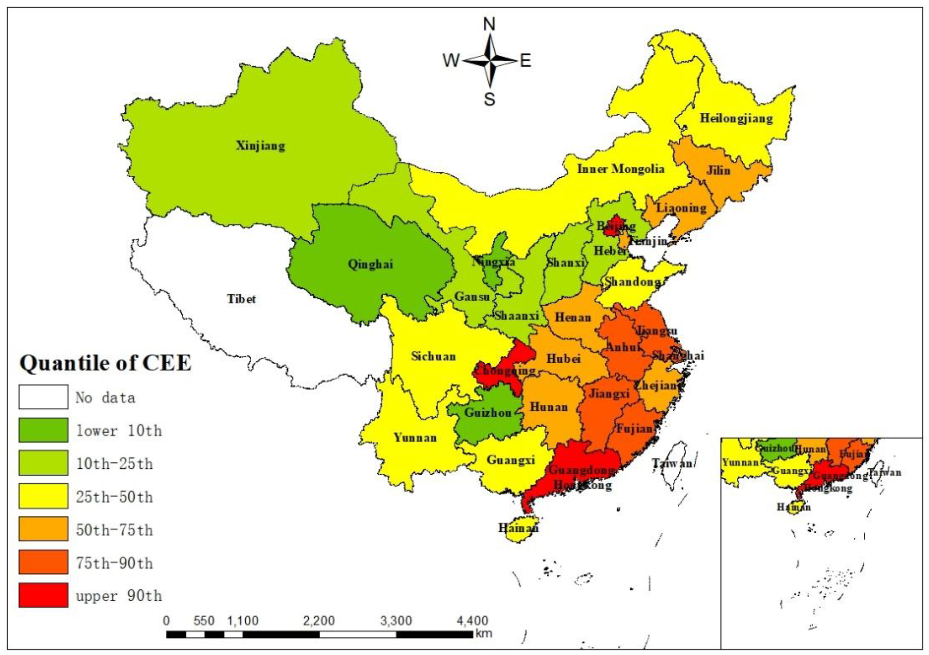
Based on Equation (6), this paper obtains the CEEs of 30 provinces in China from 2000 to 2019. The average value is only 0.172, thus indicating that the overall level of CEE is still low. Furthermore, according to the average of CEE, we choose five representative quantiles of 10%, 25%, 50%, 75%, and 90% and divide the 30 provinces into six groups (see Figure 1 and

Table A2. The grouping of China’s 30 provinces according to CEE level.

Quantile Group	Provinces
Lower 10%	Guizhou, Qinghai, Ningxia
10–25%	Shaanxi, Gansu, Hebei, Xinjiang, Shanxi
25–50%	Heilongjiang, Sichuan, Guangxi, Inner Mongolia, Hainan, Shandong, Yunnan
50–75%	Hunan, Tianjin, Hubei, Jilin, Henan, Zhejiang, Liaoning
75–90%	Fujian, Jiangxi, Anhui, Shanghai, Jiangsu
Upper 90%	Beijing, Guangdong, Chongqing

). It can be seen that roughly half of the provinces are below average, most of which are in the western region, and only Beijing, Guangdong, and Chongqing have efficiency values above the 90th quantile. From the perspective of regional distribution, provinces with higher efficiency are generally concentrated in eastern China, especially in the southeast region, and their efficiency values are significantly higher than those in the northwest region. In contrast, most northern provinces have low efficiency, especially those in the northwest, which demonstrates that there is an obvious imbalance in CEE across provinces and the spatial characteristics are very obvious.

5.2. Spatial Econometric Test

5.2.1. Spatial Autocorrelation Test

There is no doubt that CEE exhibits the spatial characteristics shown above. We further explore the spatial autocorrelation of CEE by estimating the Moran index (Moran’s I). The value of Moran’s I is typically from −1 to 1. If Moran’s I exceeds 0, then an observation has positive spatial correlation, whereas if it is less than 0, then it has negative spatial correlation. The specific formulation is as follows:

$$Moran’s I=\frac{{\displaystyle {\sum }_{i=1}^n{\displaystyle {\sum }_{j=1}^n{\omega }_{ij}}(X_i-\overline{X})(X_j-\overline{X})}}{S^2{\displaystyle {\sum }_{i=1}^n{\displaystyle {\sum }_{j=1}^n{\omega }_{ij}}}}$$

(18)

$$S^2=\frac{1}{n}{\displaystyle {\sum }_{i=1}^n(X_i}-\overline{X}{)}^2, \overline{X}=\frac{1}{n}{\displaystyle {\sum }_{i=1}^n{X}_i}$$

(19)

In Equations (18) and (19), n is the total number of regions and X_i and X_j are CEEs of regions i and j, respectively. $\overline{X}$ is the average value of all sample regions, S² is the sample variance, ${\omega }_{ij}$ is the spatial weight matrix, and ${\displaystyle {\sum }_{i=1}^n{\displaystyle {\sum }_{j=1}^n{\omega }_{ij}}}$ is the total of all spatial weights.

As shown in

Table 2. Moran’s I of carbon emission efficiency.

Year	Moran’s I	Z-Value	Year	Moran’s I	Z-Value
2000	0.445 ***	4.445	2010	0.238 **	2.501
2001	0.416 ***	4.194	2011	0.195 **	2.113
2002	0.403 ***	4.043	2012	0.218 **	2.320
2003	0.297 ***	3.065	2013	0.199 **	2.151
2004	0.322 ***	3.262	2014	0.240 **	2.519
2005	0.273 ***	2.822	2015	0.258 ***	2.684
2006	0.254 ***	2.642	2016	0.298 ***	3.052
2007	0.216 **	2.304	2017	0.304 ***	3.096
2008	0.253 ***	2.646	2018	0.304 ***	3.089
2009	0.253 ***	2.643	2019	0.277 ***	2.831

Note: **, *** denote significance at the 5% and 1% levels, respectively.

, Moran’s Is for CEE from 2000 to 2019 are all positive and significant, suggesting that CEE distribution has an apparent spatial autocorrelation.

5.2.2. Spatial Econometric Model Tests

For the analysis of the spatial econometric model, a set of estimations and statistical tests must be performed on the nonspatial panel regression model first. This indicates that the fixed effects model is more effective than the random effects model based on Hausman’s test, which rejects null hypothesis in all models (see

Table A3. Results of spatial econometric tests.

	(1)	(2)	(3)	(4)	(5)	(6)
Moran’s I	14.643 ***	14.359 ***	12.731 ***	14.704 ***	14.060 ***	12.492 ***
	(0.000)	(0.000)	(0.000)	(0.000)	(0.000)	(0.000)
LMerror	202.562 ***	194.790 ***	153.931 ***	203.825 ***	186.376 ***	147.413 ***
	(0.000)	(0.000)	(0.000)	(0.000)	(0.000)	(0.000)
R-LMerror	0.972	1.261	10.030 ***	0.835	1.681	12.166 ***
	(0.324)	(0.262)	(0.002)	(0.361)	(0.195)	(0.000)
LMlag	350.672 ***	344.478 ***	316.760 ***	349.744 ***	334.129 ***	313.562 ***
	(0.000)	(0.000)	(0.000)	(0.000)	(0.000)	(0.000)
R-LMlag	149.083 ***	150.948 ***	172.859 ***	146.753 ***	149.433 ***	178.314 ***
	(0.000)	(0.000)	(0.000)	(0.000)	(0.000)	(0.000)
SFE-LR	292.32 ***	291.95 ***	293.04 ***	287.52 ***	285.11 ***	297.88 ***
	(0.000)	(0.000)	(0.000)	(0.000)	(0.000)	(0.000)
TFE-LR	385.35 ***	389.33 ***	398.39 ***	379.64 ***	387.75 ***	398.27 ***
	(0.000)	(0.000)	(0.000)	(0.000)	(0.000)	(0.000)
Hausman	61.22 ***	64.58 ***	61.09 ***	65.78 ***	64.97 ***	57.18 ***
	(0.000)	(0.000)	(0.000)	(0.000)	(0.000)	(0.000)

Note: *** significant at the 1% level. The data in brackets are p-values.

). The two types of likelihood ratio (LR) individual and temporal effect tests pass the significance test at the 1% level, thus demonstrating that it is more appropriate that the individual and time double fixed effect model. As shown by the Lagrange multiplier test results, LMerror, R-LMerror, LMlag, and R-LMlag all pass the significance test at the 1% level, confirming Moran’s I results of the aforementioned CEE. An economic model should therefore include spatial factors as a component.

Table A4. Results of Wald and LR tests.

	(1)	(2)	(3)	(4)	(5)	(6)
Wald_lag	13.70 *	13.59 *	26.28 ***	18.06 **	21.57 ***	37.04 ***
	(0.057)	(0.059)	(0.000)	(0.021)	(0.006)	(0.000)
Wald_error	24.95 ***	24.64 ***	40.82 ***	30.88	34.93 ***	51.60 ***
	(0.001)	(0.001)	(0.000)	(0.000)	(0.000)	(0.000)
LR_lag	14.68 **	14.50 **	28.60 ***	20.31 ***	23.92 ***	39.59 ***
	(0.040)	(0.043)	(0.000)	(0.009)	(0.002)	(0.000)
LR_error	16.79 **	16.40 **	33.35 ***	23.59 ***	27.38 ***	44.78 ***
	(0.019)	(0.022)	(0.000)	(0.003)	(0.001)	(0.000)

Note: *, **, *** denote significance at the 10%, 5%, and 1% levels, respectively. The data in brackets are p-values.

presents the results of the Wald and LR tests, which both pass the significance test at the 1% level, demonstrating that the null hypothesis was rejected and SDM was not reduced to SLM and SEM. Hence, we adopt a double fixed effect SDM for subsequent empirical analysis.

5.3. Empirical Results and Discussion

The spatial lag term $\rho$ is estimated using the maximum likelihood estimation of SDM, along with the explanatory variables. The specific results are shown in

Table 3. The estimation results of SDM.

Variable	(1)	(2)	(3)	(4)	(5)	(6)
lnCE	0.0007	0.0005	0.0031	0.0011	0.0009	0.0031
	(0.133)	(0.098)	(0.574)	(0.202)	(0.160)	(0.564)
FS	0.0059			0.0107
	(0.822)			(1.207)
STOCK		0.0041			0.0102 *
		(1.127)			(1.847)
BANK			−0.0392			−0.0294
			(−1.382)			(−1.032)
lnCE×FS				0.0028 *
				(1.904)
lnCE×STOCK					0.0028 **
					(2.571)
lnCE×BANK						−0.0069
						(−0.984)
W×lnCE	0.0207 ***	0.0206 ***	0.0326 ***	0.0212 ***	0.0209 ***	0.0337 ***
	(2.666)	(2.655)	(4.021)	(2.736)	(2.731)	(4.162)
W×FS	0.0027			0.0103
	(0.270)			(0.782)
W×STOCK		0.0005			0.0132
		(0.095)			(1.438)
W×BANK			−0.1730 ***			−0.1941 ***
			(−3.350)			(−3.736)
W×lnCE×FS				0.0046 **
				(2.012)
W×lnCE×STOCK					0.0048 ***
					(2.639)
W×lnCE×BANK						−0.0376 ***
						(−3.222)
Controls	YES	YES	YES	YES	YES	YES
$\rho$	0.3151 ***	0.3173 ***	0.2207 ***	0.2905 ***	0.2765 ***	0.1727 **
	(4.989)	(5.028)	(3.295)	(4.523)	(4.275)	(2.504)
sigma2_e	0.0073 ***	0.0073 ***	0.0069 ***	0.0072 ***	0.0070 ***	0.0069 ***
	(17.434)	(17.439)	(18.065)	(17.531)	(17.785)	(17.867)
N	600	600	600	600	600	600
R2	0.1931	0.1915	0.0555	0.2336	0.2708	0.0490
Log-L	615.2968	615.4025	624.0231	619.9922	623.2845	630.6452

Note: *, **, *** denote significance at the 10%, 5%, and 1% levels, respectively. The data in brackets are t-values.

. This indicates that the local CEE is affected by a positive spatial spillover effect and that the distribution of the CEE among regions is not random, as the coefficients of $\rho$ are positive and pass the 1% significance test. The spatial distribution of regional CEE is not random.

From the empirical results shown in column (1), the coefficient of lnCE is positive but not significant, while the coefficient of W×lnCE is positive and significant, thus indicating that the positive effect of clean energy on local CEE is not obvious, but neighboring clean energy development promotes local CEE. The coefficients of FS and W×FS are both positive and nonsignificant, thus indicating that the positive effect of financial structure on CEE in local and surrounding areas is not obvious. After including lnCE×FS in column (4), the original sign and significance of lnCE and FS do not change, and the interactive coefficient is positive and passes the significance test at the 10% level, thus indicating that the combination of clean energy and the financial structure can be effective in enhancing local CEE. W×lnCE×FS is also positive and significant, thus indicating that the synergistic effect of neighboring regions can enhance local CEE.

Table 3 also shows the impact of clean energy on CEE through financial markets and bank credit. In column (5), the coefficient of lnCE×STOCK is positive and passes the significance test at the 5% level, thus illustrating that clean energy can effectively promote local CEE through the stock market, which confirms H1. W×lnCE×STOCK is also positive and significant, which indicates that neighboring clean energy generation has a positive spillover effect on local CEE through financial markets. In column (6), the coefficient of lnCE×BANK is negative and nonsignificant, thus indicating that clean energy cannot enhance local CEE through bank credit, which confirms H2. Moreover, W×lnCE×BANK is negative and significant, which reveals that neighboring clean energy generation inhibits local CEE through bank credit. The spatial spillover effect of the cointegration of clean energy and financial structure on CEE is the focus of this paper. To confirm H3, we will conduct a more in-depth empirical test.

LeSage and Pace [68] argued that the regression coefficient of SDM did not directly reflect the marginal effect of independent variables given the existence of spatial lag terms. Therefore, they decomposed the spatial effects of cross-sectional data using the partial derivative method. Then, this decomposition method was extended to spatial panel data [63]. The specific formulation of decomposition is as follows:

$$CE{E}_{it}={(I-\rho W)}^{-1}(X_{it}\alpha +W{X}_{it}\theta )+{(I-\rho W)}^{-1}{\mu }_i+{(I-\rho W)}^{-1}{\gamma }_t+{(I-\rho W)}^{-1}{\epsilon }_{it}$$

(20)

where Equation (20) is obtained by deriving explanatory variables from Equations (11)–(13). Calculating the partial derivative of the kth explanatory variable, n regions are considered, and a partial derivative matrix is generated, as shown in Equation (21):

$$[\frac{\partial CE{E}_t}{\partial X_{1k}}\cdots \frac{\partial CE{E}_t}{\partial X_{nk}}]=\left[\begin{array}{ccc}\frac{\partial CE{E}_{t1}}{\partial X_{1k}}& \cdots & \frac{\partial CE{E}_{t1}}{\partial X_{nk}}\\ ⋮& \ddots & ⋮\\ \frac{\partial CE{E}_{tn}}{\partial X_{1k}}& \cdots & \frac{\partial CE{E}_{tn}}{\partial X_{nk}}\end{array}\right]={(I-\rho W)}^{-1}\left[\begin{array}{cccc}{\beta }_k& W_{12}{\theta }_k& \cdots & W_{1n}{\theta }_k\\ W_{21}{\theta }_k& {\beta }_k& \cdots & W_{2n}{\theta }_k\\ ⋮& ⋮& \ddots & ⋮\\ W_{n1}{\theta }_k& W_{n2}{\theta }_k& \cdots & {\beta }_k\end{array}\right]$$

(21)

There are two effects in the right-hand matrix: the mean value of the main diagonal elements is direct effect, which indicates that the explanatory variable has an influence on local CEE; indirect effect occurs when the explanatory variable impacts neighboring CEEs through the mean value of nondiagonal elements. The indirect, direct, and total effects are further decomposed by using a partial derivative matrix to determine the spatial influence of independent variables on CEE. It can be seen from

Table 4. Spatial effect decomposition of SDM.

Variables	Direct Effect	Indirect Effect	Total Effect	Direct Effect	Indirect Effect	Total Effect	Direct Effect	Indirect Effect	Total Effect
lnCE	0.0026	0.0304 ***	0.0330 **	0.0023	0.0293 ***	0.0316 **	0.0044	0.0414 ***	0.0458 ***
	(0.455)	(2.797)	(2.348)	(0.401)	(2.797)	(2.317)	(0.786)	(4.444)	(3.772)
FS	0.0112	0.0193	0.0305 **
	(1.355)	(1.228)	(2.022)
STOCK				0.0109 **	0.0223 **	0.0333 ***
				(2.110)	(2.054)	(3.144)
BANK							−0.0374	−0.2366 ***	−0.2740 ***
							(−1.371)	(−3.869)	(−4.204)
GOV	−0.1933	0.4293 *	0.2360	−0.1931	0.4385 *	0.2454	−0.1661	0.7031 ***	0.5370 **
	(−1.450)	(1.789)	(0.832)	(−1.488)	(1.873)	(0.887)	(−1.226)	(3.345)	(2.158)
IS	−0.0187	−0.0020	−0.0207	−0.0219	0.0006	−0.0213	0.0066	−0.0035	0.0031
	(−0.910)	(−0.043)	(−0.350)	(−1.053)	(0.014)	(−0.373)	(0.333)	(−0.093)	(0.065)
ES	−0.2863 ***	−0.2075	−0.4937 **	−0.2801 ***	−0.2155	−0.4956 ***	−0.3130 ***	−0.1222	−0.4351 ***
	(−7.146)	(−1.132)	(−2.552)	(−7.101)	(−1.213)	(−2.645)	(−8.060)	(−0.776)	(−2.669)
TO	−0.3021 ***	−0.2349 ***	−0.5370 ***	−0.2889 ***	−0.2202 ***	−0.5091 ***	−0.3151 ***	−0.1050	−0.4201 ***
	(−7.613)	(−2.781)	(−5.527)	(−7.297)	(−2.693)	(−5.400)	(−8.182)	(−1.424)	(−5.084)
lnER	0.1314 ***	0.0587	0.1901 ***	0.1309 ***	0.0559	0.1868 ***	0.1191 ***	−0.0209	0.0981 *
	(6.509)	(1.104)	(3.176)	(6.557)	(1.081)	(3.209)	(6.005)	(−0.456)	(1.888)
lnCE×FS	0.0032 **	0.0076 **	0.0109 ***
	(2.245)	(2.453)	(2.855)
lnCE×STOCK				0.0032 ***	0.0076 ***	0.0108 ***
				(2.980)	(3.203)	(3.775)
lnCE×BANK							−0.0075	−0.0465 ***	−0.0540 ***
							(−1.108)	(−3.431)	(−3.393)

Note: *, **, *** denote significance at the 10%, 5%, and 1% levels, respectively. The data in brackets are t-values.

that the spatial effect has been decomposed to produce the results shown here.

A study has demonstrated that the direct effects of lnCE are not significant, while its indirect effects are positive and significant at the 1% level, indicating that clean energy does not have a clear impact on local CEE, while it can significantly enhance neighboring CEE via the spatial spillover effect. It is argued that clean energy is mainly reflected in power generation and has obvious spillover effects through the “west-to-east” power transmission policy formulated by the Chinese government.

FS has both direct and indirect effects that are positive but not statistically significant, which indicates that the financial structure does not impact local and neighboring CEEs. The direct and indirect effects of STOCK are 0.0109 and 0.0223, respectively, and both pass the significance at the 5% level, which demonstrates that the stock market promotes local CEE while having obvious spillover effects on neighboring regions. The direct and indirect effects of BANK are negative, which indicates that bank credit inhibits CEE in both local and neighboring areas.

The direct and indirect effects of lnCE×FS are 0.0032 and 0.0076, respectively, and both pass the significance test at the 5% level. This shows that a 1% increase in the integration of clean energy and a market-oriented financial structure leads to a 0.0032% increase in the local CEE and a 0.0076% increase in neighboring regions’ CEE through the spatial spillover effect, which confirms H3. The direct and indirect effects of lnCE×STOCK are 0.0032 and 0.0076, respectively, and both pass the significance test, which indicates that clean energy can effectively promote local and neighboring CEEs through the stock market. The direct effect of lnCE×BANK is negative but nonsignificant, while its indirect effect is negative and significant, which demonstrates not only that clean energy inhibits the local CEE through bank credit, but also that the inhibitory effect on neighboring regions is more significant. This is explained by the fact that banking institutions emphasize risk control, and clean energy is often accompanied by its own inherent uncertainties, which makes it difficult for the banking industry to provide adequate financial support for it. As for the stock market, clean energy enterprises can directly obtain social funding through the capital market, which effectively alleviates financing difficulties and enables the long-term development of clean energy to drive local economic growth and achieve carbon emission reduction. The spillover effect of clean energy and the liquidity of the financial market also encourage the surrounding areas to increase their R&D and applications of clean energy through imitation and learning to optimize their energy structure and improve their CEE.

For the control variables, the direct effects of GOV are negative but nonsignificant, while its indirect effects are positive and significant, which can be explained as follows: Local fiscal expenditure on environmental management is limited and fails to play a decisive role in the impact of local CEE, but it can play a demonstration effect for neighboring regions and help to improve the neighboring provinces’ CEE. The direct, indirect, and total effects of IS are not significant, thus indicating that upgrading the industrial structure does not have a significant impact on the local and neighboring CEEs. This is explained by the fact that tertiary industries have developed rapidly in various regions, but industrialization is still the main driving force of regional economic growth, which indicates that the transformation and upgrading of the industrial structure remains low and has not yet had a significant effect on CEE. The three effects of ES are negative, which can be explained as follows: The production processes of enterprises with high energy consumption, such as coal, will produce a large amount of carbon dioxide given China’s current energy structure. However, the downward pressure exerted by China’s slowing economy has further restrained CEE in recent years. The three effects of TO are negative and significant, thus indicating that trade openness has a significant inhibitory effect on the local and neighboring CEEs. Among the direct effects of lnER, there are significant and positive ones, demonstrating that environmental regulations play an important role in promoting local CEE. In this manner, the “innovation compensation effect” can be achieved, and local CEE can be improved by ensuring that enterprises optimize resource allocation and improve their technological levels.

5.4. Endogeneity Test

Qu and Lee [69] argue that the spatial weight matrix does not satisfy the null hypothesis that it is strictly exogenous, which may lead to endogeneity problems. The spatial lag variables W²X and W³X are used as instrumental variables in this paper to avoid endogeneity, as suggested by Zhang and Liu [60]. Among them, W denotes the space weight matrix and X indicates the explanatory variables. The specific results are shown in

Table 5. Results of the endogeneity test.

	(1)	(2)	(3)	(4)	(5)	(6)
lnCE	0.0010	0.0008	0.0033	0.0011	0.0009	0.0026
	(0.181)	(0.144)	(0.596)	(0.200)	(0.170)	(0.482)
FS	0.0059			0.0107
	(0.806)			(1.210)
STOCK		0.0037			0.0111 **
		(1.004)			(1.986)
BANK			−0.0427			−0.0218
			(−1.346)			(−0.714)
lnCE×FS				0.0028 *
				(1.844)
lnCE×STOCK					0.0026 **
					(2.398)
lnCE×BANK						−0.0052
						(−0.681)
W×lnCE	0.0243 ***	0.0237 ***	0.0340 ***	0.0209 **	0.0171 **	0.0302 ***
	(2.790)	(2.738)	(3.499)	(2.446)	(2.024)	(3.163)
W×FS	0.0027			0.0101
	(0.264)			(0.742)
W×STOCK		0.0006			0.0083
		(0.118)			(0.808)
W×BANK			−0.1825 ***			−0.1689 ***
			(−2.882)			(−2.665)
W×lnCE×FS				0.0045 *
				(1.733)
W×lnCE×STOCK					0.0035 *
					(1.788)
W×lnCE×BANK						−0.0342 ***
						(−2.694)
W×CEE	0.0512	0.0873	0.1591	0.3114	0.5328 **	0.3320
	(0.187)	(0.322)	(0.669)	(1.186)	(2.129)	(1.409)
Controls	YES	YES	YES	YES	YES	YES
Cons	0.7202 ***	0.7255 ***	0.8917 ***	0.6010 ***	0.5599 ***	0.7831 ***
	(4.329)	(4.404)	(4.941)	(3.795)	(3.626)	(4.518)
N	600	600	600	600	600	600
R2	0.8233	0.8247	0.8320	0.8335	0.8377	0.8377
Adj_R2	0.8026	0.8041	0.8122	0.8132	0.8179	0.8180
Log-L	612.5026	614.8689	627.5111	630.2494	637.9073	637.9595

Note: *, **, *** denote significance at the 10%, 5%, and 1% levels, respectively. The data in brackets are t-values.

.

There are no significant differences in the estimated coefficients of the explanatory variables (see Table 5) compared with the estimated results depicted in Table 3. Additionally, the coefficients of each variable’s spatial lag terms are similar, thereby suggesting that instrumental variables can still be used to address the endogeneity of spatial weights while maintaining consistent and robust estimation results.

5.5. Robustness Check

This paper further tests the robustness of the estimates by replacing the spatial weight matrix and changing the core explanatory variables. The results are shown in

Table 6. Results of the robustness tests.

Variables	(1)	(2)	(3)	Variables	(4)	(5)	(6)
	W01	W01	W01
lnCE	−0.0018	−0.0026	−0.0016	lnCE2	0.0059	0.0060	0.0077
	(−0.312)	(−0.457)	(−0.274)		(1.050)	(1.066)	(1.399)
FS	0.0120			FS	0.0128
	(1.404)				(1.477)
STOCK		0.0084		STOCK		0.0131 **
		(1.554)				(2.359)
BANK			−0.0607 **	BANK			−0.0293
			(−2.054)				(−1.041)
lnCE×FS	0.0026 *			lnCE2*FS	0.0030 **
	(1.738)				(1.992)
lnCE×STOCK		0.0022 **		lnCE2*STOCK		0.0033 ***
		(2.085)				(2.878)
lnCE×BANK			−0.0107	lnCE2*BANK			−0.0025
			(−1.428)				(−0.358)
W×lnCE	0.0304 ***	0.0315 ***	0.0107	W*lnCE	0.0206 **	0.0200 **	0.0339 ***
	(2.801)	(2.895)	(0.907)		(2.552)	(2.521)	(4.059)
W×FS	−0.0001			W*FS	0.0099
	(−0.006)				(0.746)
W×STOCK		0.0100		W*STOCK		0.0122
		(1.150)				(1.294)
W×BANK			0.0232	W*BANK			−0.1835 ***
			(0.438)				(−3.579)
W×lnCE×FS	0.0047 *			W*lnCE2*FS	0.0041 *
	(1.731)				(1.698)
W×lnCE×STOCK		0.0042 **		W*lnCE2*STOCK		0.0043 **
		(2.259)				(2.241)
W×lnCE×BANK			−0.0539 ***	W*lnCE2*BANK			−0.0450 ***
			(−3.356)				(−3.924)
Controls	YES	YES	YES	Controls	YES	YES	YES
$\rho$	0.1933 ***	0.1825 ***	0.1530 ***	$\rho$	0.2909 ***	0.2788 ***	0.1686 **
	(3.591)	(3.366)	(2.747)		(4.518)	(4.304)	(2.432)
sigma2_e	0.0075 ***	0.0075 ***	0.0074 ***	sigma2_e	0.0072 ***	0.0070 ***	0.0068 ***
	(17.246)	(17.260)	(17.263)		(17.532)	(17.792)	(17.863)
N	600	600	600	N	600	600	600
R2	0.2754	0.3060	0.1523	R2	0.2161	0.2540	0.0466
Log-L	612.7560	614.8708	619.2389	Log-L	619.6858	623.2532	631.7100

Note: *, **, *** denote significance at the 10%, 5%, and 1% levels, respectively. The data in brackets are t-values.

.

According to Zhang and Liu [60], this paper employs the spatial adjacent weight matrix W01 (i.e., when two regions have a common border, the weight is 1; otherwise, it is 0) as substitute matrix to investigate whether SDM will produce significantly different results due to changes in the spatial weight matrix. Compared with Table 3, there is no significant difference in the symbols and significance of the estimated coefficients using the substitute matrix in column (1), further indicating that the combination of clean energy and the financial structure can effectively enhance CEE. In column (2), the results show that clean energy can still effectively improve local and neighboring CEEs through stock market. In column (3), the results show that the interaction between clean energy and bank credit has a dampening effect on local and neighboring CEEs.

Nuclear energy is controversial in its ability to promote economic development and reduce CO₂ emissions [28] compared with other types of clean energy. Additionally, it may threaten living conditions due to safety issues that have arisen in recent years. Following Chen et al. [9], we exclude nuclear power from the clean energy indicators used in this paper and construct a new proxy variable, lnCE2, to perform a robustness test. There is no significant difference between the estimates in Table 3 and the findings in this study. For example, the coefficient of lnCE2×FS is 0.0030 (p < 0.05), which indicates that it still contributes to CEE. The coefficients of lnCE2×STOCK and W×lnCE2×STOCK are positive and significant, thus indicating that they improve the local and neighboring CEEs, while lnCE2×BANK and W×lnCE2×BANK are negative and similar to the results shown in Table 5. Therefore, the estimation results are strongly robust.

5.6. Spatial Quantile Regression Results

The average effect of combining clean energy and financial structures to affect CEE is mainly obtained through the abovementioned empirical studies. Under various provinces’ CEE, this paper seeks to identify the characteristics of clean energy interaction with a market-oriented financial structure by using SQR and the 10th, 25th, 50th, 75th, and 90th quantiles for analysis. As shown in

Table 7. Estimation results of SQR.

	10th	25th	50th	75th	90th
W×CEE	0.0874	0.1028	0.2378	0.2987 **	0.2318 ***
	(1.007)	(0.960)	(1.411)	(2.463)	(2.904)
lnCE	0.0006	−0.0039	−0.0082	−0.0003	0.0085
	(0.150)	(−0.721)	(−1.066)	(−0.040)	(1.121)
FS	0.0111	0.0186 **	0.0197 *	0.0179 *	0.0157 *
	(1.558)	(2.030)	(1.657)	(1.768)	(1.743)
lnCE×FS	0.0010	0.0023	0.0030	0.0029 *	0.0032 *
	(0.885)	(1.598)	(1.532)	(1.675)	(1.843)
W×lnCE	0.0089	0.0104	−0.0020	0.0173	0.0188 *
	(0.979)	(0.951)	(−0.158)	(1.422)	(1.899)
W×FS	0.0023	−0.0020	0.0141	0.0095	0.0132
	(0.210)	(−0.146)	(0.914)	(0.789)	(0.959)
W×lnCE×FS	0.0011	0.0026	0.0036	0.0038 *	0.0040 *
	(0.461)	(0.859)	(1.192)	(1.737)	(1.811)
Controls	YES	YES	YES	YES	YES
Individual fixed	YES	YES	YES	YES	YES
Time fixed	YES	YES	YES	YES	YES
Cons	0.1421	0.1319	0.3165	0.6039 **	0.7047 ***
	(1.506)	(1.096)	(1.471)	(2.519)	(2.912)
N	600	600	600	600	600

Note: *, **, *** denote significance at the 10%, 5%, and 1% levels, respectively. The data in brackets are t-values.

, the estimated results are presented.

The coefficients of lnCE×FS are positive at all five quartiles, and the coefficient of the 90th quantile is 0.0032 and passes the significance test at the 10% level, while the 10th quantile is the smallest at only 0.0010. This indicates that the interaction between clean energy and a market-oriented finance can enhance CEE in various regions, and this synergistic effect is more significant in areas with higher efficiency. Accordingly, it can be concluded that clean energy impacts CEE differently in different provinces with market-oriented financial structures. Additionally, with the increase in CEE, the coefficient of W×lnCE×FS is also increased, and the coefficient of the 90th quantile reaches its maximum and is significant, which demonstrates that the impact of clean energy through a market-oriented financial structure in neighboring areas increases with the continued growth of local CEE.

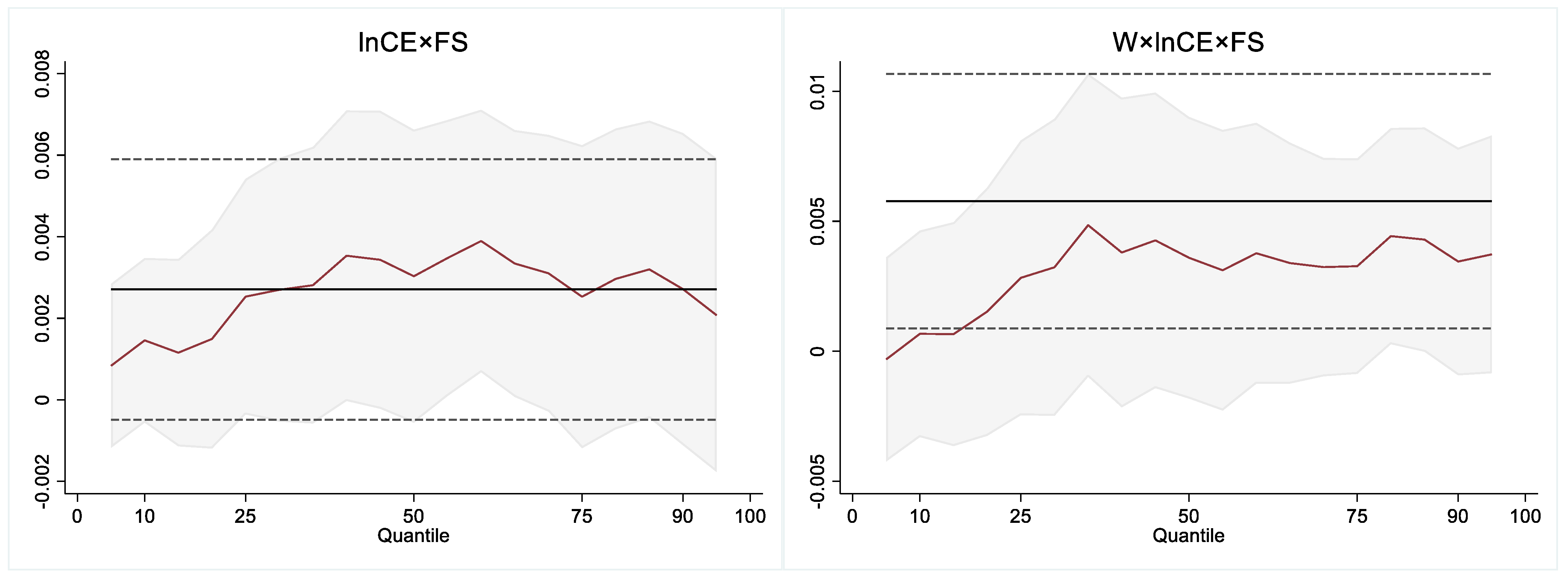
This paper plots the regression coefficients of lnCE×FS and W×lnCE×FS at all quartiles, which allows for a more intuitive description of the dynamic trajectory of the joint impacts of clean energy and the financial structures on CEE (see Figure 2). It can be seen that the change in the coefficient of lnCE×FS is similar to an “inverted U-shaped” pattern, and its interactive coefficient represents a fluctuating upward trend in the 10th–50th quantiles, while it shows a downward trend to some extent from the 50th to the 90th quantiles. The coefficient of W×lnCE×FS shows an upward trend. Among them, the coefficient of the 5th quantile is the lowest and less than 0, and the coefficients above the 25th quantile are all greater than 0 and increasing. This indicates that the neighboring provinces’ clean energy production inhibits local CEE through market-oriented finance in regions with low efficiency (e.g., Guizhou, Qinghai, and Ningxia), while the positive role of neighboring regions will gradually increase in areas with higher efficiency. This is consistent with the estimates shown in Table 7, where clean energy enhances local CEE through a market-oriented financial structure and the effect varies. With the increase in CEE, the stimulating effect, by which clean energy is supported by a market-oriented financial structure in neighboring areas, is gradually enhanced.

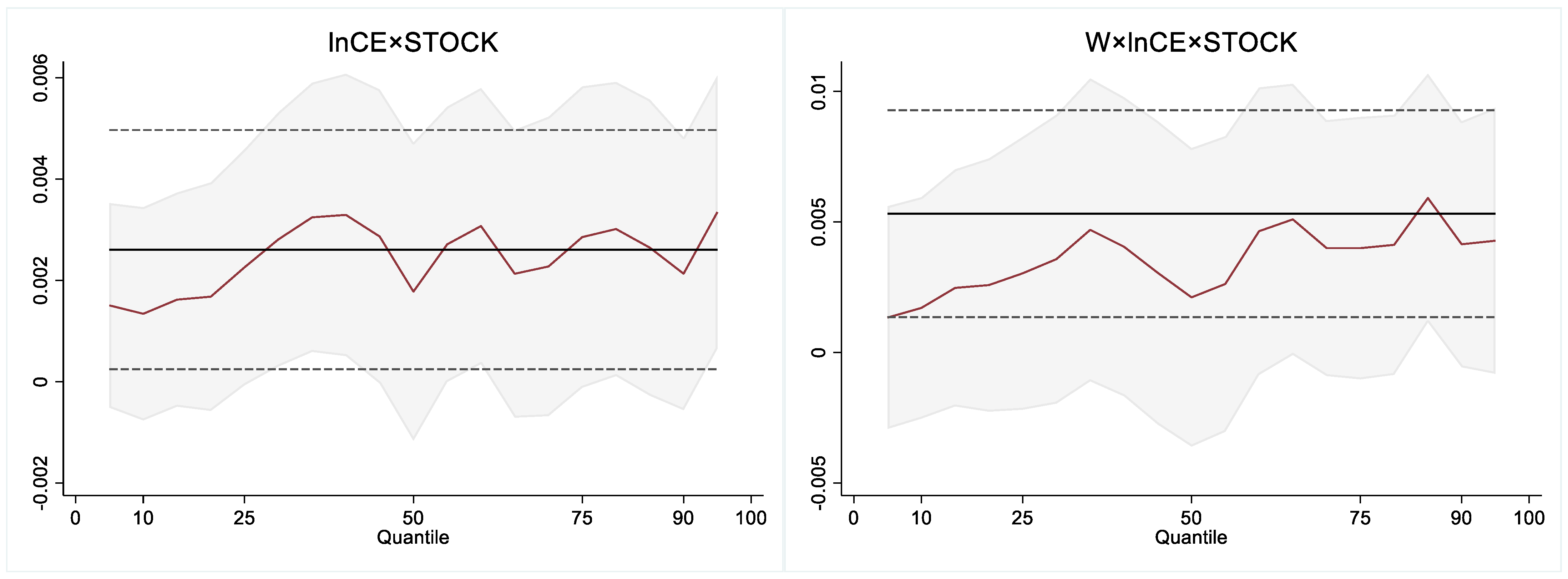
Furthermore, this paper plots the trend of the coefficients of lnCE×STOCK and W×lnCE×STOCK at all quantiles (see Figure 3). As a whole, the coefficient of lnCE×STOCK is positive, which indicates that clean energy can enhance CEE through the stock market in all regions. The coefficients are relatively small before the 25th quantile, thus indicating that clean energy does not significantly improve CEE through the stock market in low-efficiency areas, such as Hebei, Xinjiang, Shanxi, Guizhou, Qinghai, and Ningxia. This is explained by the fact that these provinces are concentrated in the western district, where fewer clean energy companies are located and are not supported by the financial market. Meanwhile, they are rich in fossil energy resources, and the substitution effect of clean energy is not fully reflected in the local economy, which is not effective in promoting CEE. When CEE increases, there is evident volatility between the 25th and 90th quantiles, indicating that clean energy and the stock market interact differently. It is explained by the fact that different regions possess substantially different resources and financial markets. Some western provinces with high economic development, such as Sichuan, are not only relatively rich in natural resources, but also have a number of listed energy companies to support clean energy development through capital markets to improve the local economy and reduce CO₂ emissions. For regions with higher economic development, the financial market is relatively mature, but the huge demand for energy and the relative lack of natural resources increase the competition for clean energy among regions, which leads to the impact of clean energy through direct financing being unsatisfactory.

The coefficient of W×lnCE×STOCK shows a fluctuating upward trend. From the 10th to the 25th quantiles, the coefficients are relatively small, while their coefficients show higher volatility from the 25th to the 90th quantiles. This indicates that the interactive effect between clean energy and the stock market on local CEE is not obvious in the low-efficiency regions, while the neighboring provinces’ clean energy has significant spillover effects through the stock market in the higher-efficiency regions, although the differences between them are large. A possible explanation for this finding is that the cross-regional liquidity of the stock market provides financial support for clean energy development in the surrounding regions and thus improves the neighboring provinces’ CEE. As CEE rises, local governments work to develop clean energy but lack planning and coordination, which aggravates competition among provinces. Therefore, the interaction between the two is highly volatile.

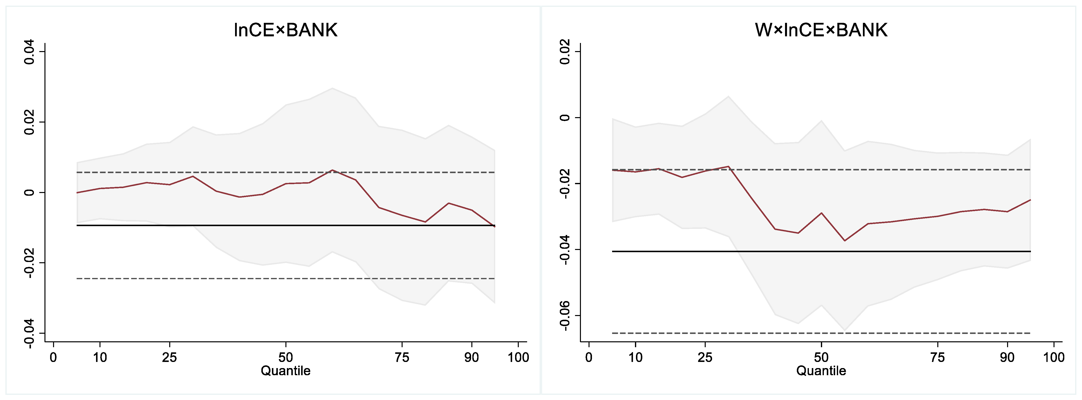
Figure 4 shows the trends in lnCE×BANK and W×lnCE×BANK. The coefficients of lnCE×BANK are less than 0 in most quantiles and obviously decrease from the 50th to the 90th quantiles, which indicates that clean energy has a mitigating effect on CEE via bank credit in most provinces, especially in high-efficiency areas. A possible explanation for this finding is that clean energy development is faced with problems such as small scales, high development costs, and longer payback periods. Meanwhile, considering the influence of natural endowments and immature clean energy technologies, banks and financial institutions are more willing to provide financing facilities for state-owned enterprises due to risk aversion in regions with high economic levels (e.g., Beijing, Guangdong, and Chongqing), while they are very cautious in providing financial support for clean energy enterprises.

As a whole, the coefficients of W×lnCE×BANK are less than 0. From the 10th to the 25th quantiles, they show a relatively steady trend, then decrease rapidly from the 25th to the 50th quantiles, and then remain low after the 50th quantile. This demonstrates that the neighboring regions’ clean energy generation suppresses the local CEE through bank credit. In the low-efficiency regions, the inhibitory effect of neighboring areas is lower, while it is more obvious in high-efficiency regions.

6. Conclusions and Policy Implications

This study analyzes the influencing mechanism of clean energy on CEE through market-oriented financial structures to fill the research gap in this area. Based on the panel data of 30 provinces in China from 2000 to 2019, this paper employs the improved NDDF to calculate the CEE of each province and applies SDM to empirically investigate the relationship between clean energy, financial structure, and CEE. Furthermore, we also apply SQR to conduct a heterogeneity analysis according to the regional division of CEE. We obtain several interesting conclusions.

6.1. Conclusions

(1) It is evident that the provincial CEE in China is spatially autocorrelative, and the local CEE is spatially positively correlated with neighboring regions. (2) A 1% increase in the integration of clean energy and market-oriented financial structure leads to a 0.0032% increase in the local CEE and a 0.0076% increase in neighboring regions’ CEE through the spatial spillover effect. The regression results of SDM are strongly robust through the endogeneity and robustness tests. Among those, clean energy impacts local CEEs positively through the stock market and significantly spatially through spillover effects to surrounding provinces, while inhibiting local and neighboring CEEs through bank credit. (3) Under the market-oriented financial structure, clean energy enhances the local CEE in all quantiles, and the impact of neighboring areas will increase gradually as the local CEE rises. From the 25th to the 90th quantiles, clean energy can greatly promote CEE through the capital market, and neighboring regions also show significant spillover effects. While the interactive effect between clean energy and bank credit suppresses the local CEE in most provinces, the inhibitory effect of neighboring regions is obvious.

6.2. Policy Implications

First, a long-term coordination mechanism should be established between regions to enhance CEE. Each provincial government should set up a coordination and leadership group to explore the balance between regional economic development and carbon emission reduction and to provide regional policy guarantee to achieve the dual goals of carbon peaking and carbon neutrality.

Second, clean energy development should be provided with more effective financial services in order to promote CEE. The central government should improve the upper-level design of the financial system, and local governments should formulate more detailed regulations to guide the flow of funds to the clean energy industry. All regions should give full play to the spatial spillover effect of clean energy and the cross-regional mobility of financial resources, and effectively integrate the two to enhance the overall CEE in China.

Third, policy makers should create support plans for clean energy that are individualized to the conditions of the local region in order to alleviate the imbalances in CEE across the country. Each local government should adopt differentiated policies and formulate targeted financial measures according to the CEE in different regions to improve the efficiency of regional clean energy capital allocation.

6.3. Discussion

Unlike the existing literature, this paper explores the spatial effects of clean energy and a financial structure on the efficiency of carbon emissions in Chinese provinces. Dong et al. [10] argued that clean energy could be effective in enhancing CEE when financial development exceeds the threshold value. Unlike them, this study finds that the integration of clean energy with a market-oriented financial structure not only improves local CEE, but also has spillover effects on neighboring regions. In addition, Yu [12] analyzed the heterogeneity of a financial structure affecting carbon emission intensity by dividing each region according to administrative regions. Based on the difference of CEE, this study applies the SQR model for heterogeneity analysis, avoiding the subjective factor of administrative region grouping.

At present, this paper uses provincial-level data, which can be followed by collecting firm panel data to explore the impact of the financing structure of clean energy firms on carbon efficiency from a more microscopic perspective. Additionally, this paper just only analyzes the average effect of a certain study sample by a spatial econometric model, and cannot obtain the heterogeneity influence of clean energy and financial structure on CEE in each region. The panel geographically and temporally weighted regression model can be used for further research.

References

1. Fan, M.; Shao, S.; Yang, L. Combining global Malmquist-Luenberger index and generalized method of moments to investigate industrial total factor CO2 emission performance: A case of Shanghai (China). Energy Policy 2015, 79, 189–201. [Google Scholar] [CrossRef]
2. Xu, L.; Fan, M.; Yang, L.; Shao, S. Heterogeneous green innovations and carbon emission performance: Evidence at China’s city level. Energy Econ. 2021, 99, 105269. [Google Scholar] [CrossRef]
3. Du, K.; Li, J. Towards a green world: How do green technology innovations affect total-factor carbon productivity. Energy Policy 2019, 131, 240–250. [Google Scholar] [CrossRef]
4. Zeng, S.; Su, B.; Zhang, M.; Gao, Y.; Liu, J.; Luo, S.; Tao, Q. Analysis and forecast of China’s energy consumption structure. Energy Policy 2021, 159, 112630. [Google Scholar] [CrossRef]
5. Balsalobre-Lorente, D.; Shahbaz, M.; Roubaud, D.; Farhani, S. How economic growth, renewable electricity and natural resources contribute to CO2 emissions? Energy Policy 2018, 113, 356–367. [Google Scholar] [CrossRef]
6. Dogan, E.; Altinoz, B.; Madaleno, M.; Taskin, D. The impact of renewable energy consumption to economic growth: A replication and extension of Inglesi-Lotz (2016). Energy Econ. 2020, 90, 104866. [Google Scholar] [CrossRef]
7. Cai, Y.; Sam, C.Y.; Chang, T. Nexus between clean energy consumption, economic growth and CO2 emissions. J. Clean. Prod. 2018, 182, 1001–1011. [Google Scholar] [CrossRef]
8. Charfeddine, L.; Kahia, M. Impact of renewable energy consumption and financial development on CO2 emissions and economic growth in the MENA region: A panel vector autoregressive (PVAR) analysis. Renew. Energy 2019, 139, 198–213. [Google Scholar] [CrossRef]
9. Chen, Y.; Shao, S.; Fan, M.; Tian, Z.; Yang, L. One man’s loss is another’s gain: Does clean energy development reduce CO2 emissions in China? Evidence based on the spatial Durbin model. Energy Econ. 2022, 107, 105852. [Google Scholar] [CrossRef]
10. Dong, F.; Li, Y.; Gao, Y.; Zhu, J.; Qin, C.; Zhang, X. Energy transition and carbon neutrality: Exploring the non-linear impact of renewable energy development on CEE in developed countries. Resour. Conserv. Recycl. 2022, 177, 106002. [Google Scholar] [CrossRef]
11. Wen, S.; Lin, B.; Zhou, Y. Does financial structure promote energy conservation and emission reduction? Evidence from China. Int. Rev. Econ. Financ. 2021, 76, 755–766. [Google Scholar] [CrossRef]
12. Yu, Y. The impact of financial system on carbon intensity: From the perspective of digitalization. Sustainability 2023, 15, 1314. [Google Scholar] [CrossRef]
13. Shen, Y.; Su, Z.W.; Malik, M.Y.; Umar, M.; Khan, Z.; Khan, M. Does green investment, financial development and natural resources rent limit carbon emissions? A provincial panel analysis of China. Sci. Total Environ. 2021, 755, 142538. [Google Scholar] [CrossRef]
14. Ji, Q.; Zhang, D. How much does financial development contribute to renewable energy growth and upgrading of energy structure in China? Energy Policy 2019, 128, 114–124. [Google Scholar] [CrossRef]
15. Chen, S. The abatement of carbon dioxide intensity in China: Factors decomposition and policy implications. World Econ. 2011, 34, 1148–1167. [Google Scholar] [CrossRef]
16. Ferreira, A.; Pinheiro, M.D.; de Brito, J.; Mateus, R. Combined carbon and energy intensity benchmarks for sustainable retail stores. Energy 2018, 165, 877–889. [Google Scholar] [CrossRef]
17. Zhou, P.; Ang, B.; Han, J. Total factor carbon emission performance: A Malmquist index analysis. Energy Econ. 2010, 32, 194–201. [Google Scholar] [CrossRef]
18. Du, K.; Lin, B. International comparison of total-factor energy productivity growth: A parametric Malmquist index approach. Energy 2017, 118, 481–488. [Google Scholar] [CrossRef]
19. Zhou, P.; Ang, B.; Wang, H. Energy and CO2 emission performance in electricity generation: A non-radial directional distance function approach. Eur. J. Oper. Res. 2012, 221, 625–635. [Google Scholar] [CrossRef]
20. Du, K.; Lu, H.; Yu, K. Sources of the potential CO2 emission reduction in China: A nonparametric meta-frontier approach. Appl. Energy 2014, 115, 491–501. [Google Scholar] [CrossRef]
21. Cheng, Z.; Liu, J.; Li, L.; Gu, X. Research on meta-frontier total-factor energy efficiency and its spatial convergence in Chinese provinces. Energy Econ. 2020, 86, 104702. [Google Scholar] [CrossRef]
22. Dong, F.; Zhu, J.; Li, Y.; Chen, Y.; Gao, Y.; Hu, M.; Qin, C.; Sun, J. How green technology innovation affects CEE: Evidence from developed countries proposing carbon neutrality targets. Environ. Sci. Pollut. Res. 2022, 29, 35780–35799. [Google Scholar] [CrossRef]
23. Cheng, Z.; Li, L.; Liu, J.; Zhang, H. Total-factor CEE of China’s provincial industrial sector and its dynamic evolution. Renew. Sustain. Energy Rev. 2018, 94, 330–339. [Google Scholar] [CrossRef]
24. Wang, K.; Wu, M.; Sun, Y.; Shi, X.; Sun, A.; Zhang, P. Resource abundance, industrial structure, and regional carbon emissions efficiency in China. Resour. Policy 2019, 60, 203–214. [Google Scholar] [CrossRef]
25. Wu, S.; Zhang, K. Influence of Urbanization and Foreign Direct Investment on Carbon Emission Efficiency: Evidence from Urban Clusters in the Yangtze River Economic Belt. Sustainability 2021, 13, 2722. [Google Scholar] [CrossRef]
26. Lee, J.W. Long-run dynamics of renewable energy consumption on carbon emissions and economic growth in the European union. Int. J. Sustain. Dev. World Ecol. 2019, 26, 69–78. [Google Scholar] [CrossRef]
27. Salim, R.; Hassan, K.; Shafiei, S. Renewable and non-renewable energy consumption and economic activities: Further evidence from OECD countries. Energy Econ. 2014, 44, 350–360. [Google Scholar] [CrossRef]
28. Azam, A.; Rafiq, M.; Shafique, M.; Zhang, H.; Yuan, J. Analyzing the Effect of Natural Gas, Nuclear Energy and Renewable Energy on GDP and Carbon Emissions: A multi-variate Panel Data analysis. Energy 2020, 219, 119592. [Google Scholar] [CrossRef]
29. Zheng, H.; Song, M.; Shen, Z. The evolution of renewable energy and its impact on carbon reduction in China. Energy 2021, 237, 121639. [Google Scholar] [CrossRef]
30. Paramati, S.R.; Ummalla, M.; Apergis, N. The effect of foreign direct investment and stock market growth on clean energy use across a panel of emerging market economies. Energy Econ. 2016, 56, 29–41. [Google Scholar] [CrossRef]
31. Raghutla, C.; Shahbaz, M.; Chittedi, K.R.; Jiao, Z. Financing clean energy projects: New empirical evidence from major investment countries. Renew. Energy 2021, 169, 231–241. [Google Scholar] [CrossRef]
32. Yu, S.; Hu, X.; Li, L.; Chen, H. Does the development of renewable energy promote carbon reduction? Evidence from Chinese provinces. J. Environ. Manag. 2020, 268, 110634. [Google Scholar] [CrossRef]
33. Liu, G.; Zhang, C. Does financial structure matter for economic growth in China. China Econ. Rev. 2020, 61, 101194. [Google Scholar] [CrossRef]
34. Inglesi-Lotz, R. The impact of renewable energy consumption to economic growth: A panel data application. Energy Econ. 2016, 53, 58–63. [Google Scholar] [CrossRef]
35. Wang, Q.; Wang, L. Renewable energy consumption and economic growth in OECD countries: A nonlinear panel data analysis. Energy 2020, 207, 118200. [Google Scholar] [CrossRef]
36. Chen, C.; Pinar, M.; Stengos, T. Renewable energy consumption and economic growth nexus: Evidence from a threshold model. Energy Policy 2020, 139, 111295. [Google Scholar] [CrossRef]
37. Bhattacharya, M.; Paramati, S.; Bhattacharya, S. The effect of renewable energy consumption on economic growth: Evidence from top 38 countries. Appl. Energy 2016, 162, 733–741. [Google Scholar] [CrossRef]
38. Qi, T.; Zhang, X.; Karplus, V. The energy and CO2 emissions impact of renewable energy development in China. Energy Policy 2014, 68, 60–69. [Google Scholar] [CrossRef]
39. Menyah, K.; Wolde-Rufael, Y. CO2 emissions, nuclear energy, renewable energy and economic growth in the US. Energy Policy 2010, 38, 2911–2915. [Google Scholar] [CrossRef]
40. Baum, C.F.; Schäfer, D.; Talavera, O. The impact of the financial system’s structure on firms’ financial constraints. J. Int. Money Financ. 2011, 30, 678–691. [Google Scholar] [CrossRef]
41. Kim, D.; Lin, S.; Chen, T. Financial structure, firm size and industry growth. Int. Rev. Econ. Financ. 2016, 41, 23–39. [Google Scholar] [CrossRef]
42. Levine, R. Stock markets, growth, and tax policy. J. Financ. 1991, 46, 1445–1465. [Google Scholar] [CrossRef]
43. Yeh, C.; Huang, H.; Lin, P. Financial structure on growth and volatility. Econ. Model. 2013, 35, 391–400. [Google Scholar] [CrossRef]
44. Demir, A.U.; Hall, S.G. Financial structure and economic development: Evidence on the view of ‘new structuralism’. Int. Rev. Financ. Anal. 2017, 52, 252–259. [Google Scholar] [CrossRef]
45. Allen, F.; Bartiloro, L.; Gu, X.; Kowalewksi, O. Does economic structure determine financial structure? J. Int. Econ. 2018, 114, 389–409. [Google Scholar] [CrossRef]
46. Yao, X.; Tang, X. Does financial structure affect CO2 emissions? Evidence from G20 countries. Financ. Res. Lett. 2020, 41, 101791. [Google Scholar] [CrossRef]
47. Matemilola, B.T.; Banyariffin, A.N.; Azmansaini, W.N.; Nassir, A.M. Impact of institutional quality on the capital structure of firms in developing countries. Emerg. Mark. Rev. 2019, 39, 175–209. [Google Scholar] [CrossRef]
48. Hsu, P.H.; Tian, X.; Xu, Y. Financial development and innovation: Cross-country evidence. J. Financ. Econ. 2014, 112, 116–135. [Google Scholar] [CrossRef]
49. Mishra, D.R. Post-innovation CSR performance and firm value. J. Bus. Ethics 2017, 140, 285–306. [Google Scholar] [CrossRef]
50. Guo, S.; Jiang, Z.; Shi, H. The business cycle implications of bank discrimination in China. Econ. Model. 2018, 73, 264–278. [Google Scholar] [CrossRef]
51. Nasir, M.A.; Huynh, T.L.D.; Tram, H.T.X. Role of financial development, economic growth & foreign direct investment in driving climate change: A case of emerging ASEAN. J. Environ. Manag. 2019, 242, 131–141. [Google Scholar] [CrossRef]
52. Shan, Y.; Guan, D.; Hubacek, K.; Zheng, B.; Davis, S.J.; Jia, L.; Liu, J.; Liu, Z.; Fromer, N.; Mi, Z.; et al. City-level climate change mitigation in China. Sci. Adv. 2018, 4, 190027. [Google Scholar] [CrossRef]
53. Chica-Olmo, J.; Sari-Hassoun, S.; Moya-Fernández, P. Spatial relationship between economic growth and renewable energy consumption in 26 European countries. Energy Econ. 2020, 92, 104962. [Google Scholar] [CrossRef]
54. Färe, R.; Grosskopf, S.; Lovell, C.A.K.; Pasurka, C. Multilateral productivity comparisons when some outputs are undesirable: A nonparametric approach. Rev. Econ. Stat. 1989, 71, 90–98. [Google Scholar] [CrossRef]
55. Battese, G.E.; Rao, D.S.P.; O’Donnell, C.J. A Metafrontier Production Function for Estimation of Technical Efficiencies and Technology Gaps for Firms Operating Under Different Technologies. J. Product. Anal. 2004, 21, 91–103. [Google Scholar] [CrossRef]
56. O’Donnell, C.J.; Rao, D.S.P.; Battese, G.E. Metafrontier frameworks for the study of firm-level efficiencies and technology ratios. Empir. Econ. 2008, 34, 231–255. [Google Scholar] [CrossRef]
57. Chambers, R.G.; Chung, Y.; Färe, R. Benefit and distance functions. J. Econ. Theory 1996, 70, 407–419. [Google Scholar] [CrossRef]
58. Fukuyama, H.; Weber, W.L. A directional slacks-based measure of technical efficiency. Socioecon. Plan. Sci. 2009, 43, 274–287. [Google Scholar] [CrossRef]
59. Zhang, N.; Choi, Y. Total-factor carbon emission performance of fossil fuel power plants in China: A metafrontier non-radial Malmquist index analysis. Energy Econ. 2013, 40, 549–559. [Google Scholar] [CrossRef]
60. Zhang, M.; Liu, Y. Influence of digital finance and green technology innovation on China’s CEE: Empirical analysis based on spatial metrology. Sci. Total Environ. 2022, 838, 156463. [Google Scholar] [CrossRef]
61. Liu, X.; Liu, X. Can financial development curb carbon emissions? Empirical test based on Spatial perspective. Sustainability 2021, 13, 11912. [Google Scholar] [CrossRef]
62. Elhorst, J.P.; Lacombe, D.J.; Piras, G. On model specification and parameter space definitions in higher order spatial econometric models. Reg. Sci. Urban Econ. 2012, 42, 211–220. [Google Scholar] [CrossRef]
63. Elhorst, J.P. Spatial Econometrics: From Cross-Sectional Data to Spatial Panels; Springer: Berlin/Heidelberg, Germany, 2014. [Google Scholar]
64. Beck, T.; Levine, R. Industry Growth and Capital Allocation: Does Having a Market-or Bank-based System Matter. J. Financ. Econ. 2002, 64, 147–180. [Google Scholar] [CrossRef]
65. Taskin, F.; Zaim, O. The role of international trade on environmental efficiency: A DEA approach. Econ. Model. 2001, 18, 1–17. [Google Scholar] [CrossRef]
66. Long, R.; Gan, X.; Chen, H.; Wang, J.; Li, Q. Spatial econometric analysis of foreign direct investment and carbon productivity in China: Two-tier moderating roles of industrialization development. Resour. Conserv. Recycl. 2020, 155, 104677. [Google Scholar] [CrossRef]
67. Huang, D. Green finance, environmental regulation, and regional economic growth: From the perspective of low-carbon technological progress. Environ. Sci. Pollut. Res. 2022, 29, 33698–33712. [Google Scholar] [CrossRef]
68. Lesage, J.P.; Pace, R.K. Introduction to Spatial Econometrics; CRC Press Taylor & Francis Group: Boca Raton, FL, USA, 2009; Available online: https://link.springer.com/article/10.1007/BF03354894 (accessed on 14 May 2015).
69. Qu, X.; Lee, L. Estimating a spatial autoregressive model with an endogenous spatial weight matrix. J. Econom. 2015, 184, 209–232. [Google Scholar] [CrossRef]
Figure 1. Average carbon emission efficiency of 30 provinces in China from 2000 to 2019.
Sustainability 15 03339 g001
Figure 2. Quantile distribution of interactive coefficients between clean energy and the financial structure.
Sustainability 15 03339 g002
Figure 3. Quantile distribution of the interactive coefficients between clean energy and stock market.
Sustainability 15 03339 g003
Figure 4. Quantile distribution of interaction term coefficients for clean energy and bank credit.
Sustainability 15 03339 g004