1. Introduction
With the development of intelligent traffic systems, traffic flow prediction has become an important and challenging topic of research in both academia and industry. The objective of intelligent traffic systems is to increase the efficiency of traffic operations and alleviate traffic congestion [
1]. It is also used as an important reference for vehicle route planning [
2] and an important topic of discussion for intelligent transportation systems [
3]. Traffic flow prediction serves as a crucial foundation for traffic demand policies in intelligent transportation systems. It enables the prediction of traffic flow in congested areas, facilitating the efficient utilization of traffic resources and contributing to sustainable traffic development at an economic level [
4]. Furthermore, the deployment of ITS technology for traffic flow prediction can aid in reducing pollution emissions that result from traffic energy consumption and congestion. This is achieved by promoting the use of public transportation and providing transportation services to those who are transportation disadvantaged.
However, traffic flow prediction is not an easy task. Traffic flow must reflect both temporal and spatial features in the presence of various variables and many uncertain factors [
5]. Therefore, it has numerous inflection points. In addition, traffic flow values may differ from the expected values because of special events (e.g., traffic accidents). An inaccurate prediction can lead to the mismanagement of traffic, potentially resulting in safety hazards [
6]. Particularly in scenarios such as traffic congestion or special events, a slight misjudgment can escalate into significant safety concerns [
7]. As such, extensive research on the prediction of traffic flow using deep learning has been conducted because it is difficult to express the values using specific formulas [
8,
9,
10]. With rapid urbanization and an increase in vehicular traffic, ensuring the safety of road users has become paramount [
11]. Accurate traffic flow prediction not only aids in efficient traffic management, but also plays a crucial role in enhancing road safety by anticipating and mitigating potential traffic hazards [
12].
Recent studies have highlighted approaches that fall into three predominant categories based on the techniques, as depicted in
Figure 1: traditional techniques, machine learning, and deep learning. These techniques are representative of the conventional strategies that are deeply anchored in knowledge-driven processes.
Before the advent of machine and deep learning, traffic flow was primarily predicted using traditional methodologies. These primarily encompass time series models, such as autoregressive integrated moving average (ARIMA) models [
13], simulation models [
14], and the Kalman filtering technique [
15]. Head [
14] used a simulation model to predict traffic, highlighting that proactive methods can be used to generate conventional real-time responses [
14], and Necula [
16] also used a simulation model based on GPS data [
16]. These traditional methodologies are the basis for traffic flow prediction; however, they are less accurate than other current methods [
17]. Although they can extract temporal features from a time series, they have difficulty expressing spatial relationships in traffic flow prediction tasks [
18]. Several researchers have proposed a combination of these methods and artificial intelligence (AI) models to address these problems.
Moreover, with advancements in machine learning and the growth in computing power, researchers have attempted to predict traffic flow using various machine learning-based models [
19], including support vector regression [
20] and K-nearest neighbor (KNN) [
21]. Tempelmeier et al. [
21] utilized the KNN algorithm to introduce a map model that captures the spatial and temporal dependencies in traffic flow data, considering the frequency of events [
21].
Recently, several models have been introduced to reflect the time series features of traffic, such as recurrent neural networks, long short-term memory (LSTM), and gated recurrent units (GRUs) based on deep learning, including models of graphs and convolutional neural networks (CNNs), such as temporal graph convolutional networks [
22] and diffusion convolutional recurrent neural networks [
23], which have been used to reflect spatial information. The emergence of these models has improved the performance of traffic flow prediction [
22,
23,
24,
25]. In the case of CNNs, traffic flow prediction is achieved by incorporating spatial characteristics via filters. Although they demonstrated effective performance in short-term predictions, they struggled to capture time series characteristics as effectively as they did spatial characteristics, leading to limitations in long-term predictions [
26]. To address these limitations, RNN-based models that reflect time series characteristics have been developed. However, traditional RNN models face a vanishing gradient problem. As a solution, LSTM and GRU models have been developed to counteract this issue [
27]. Lu et al. [
28] identified the shortcomings in prevailing traffic flow prediction models that fail to capture high-level temporal patterns. To address this, they integrated stacked LSTM blocks with convolutional blocks [
28]. The introduction of GRUs has further mitigated the vanishing gradient challenge. R. Fu et al. [
19] conducted an experiment on short-term traffic flow prediction using LSTM and GRUs, revealing that the deep learning approach, based on current neural networks, such as RNN, surpassed traditional time series models such as ARIMA in capturing temporal nuances [
19]. Nonetheless, because traffic flow prediction encompasses both spatial and temporal properties, there is a demand for models that can effectively represent both dimensions. To this end, a temporal convolution network was designed to reflect both time series and spatial features. This model efficiently addresses the issues of computational time and the vanishing gradient problem inherent to traditional RNNs, and its performance can be optimized by adjusting the layer count and tweaking the parameters. It outperformed the traditional LSTM, GRU, and RNN models [
29].
Consequently, a plethora of models are continually being developed to enhance prediction accuracy and streamline traffic flow forecasting. However, most studies on traffic flow prediction have focused on prediction accuracy. However, they did not provide information regarding the reliability of the prediction. The performance of the model is evaluated using various evaluation metrics, such as the root mean square error (RMSE) and R-squared; however, they only indicate the performance of the average for past data. They did not provide information on the reliability of the predicted value through the model at the prediction stage through the actual model. This can lead to misjudgment, thus acting as an obstacle to better decision making and deviating from the ultimate goal of deep learning models. In previous studies, this problem was solved using uncertainty [
30,
31,
32]. Uncertainty is the reliability of the model in regard to the predicted result value. The higher the uncertainty, the lower the reliability of the predicted value, and the higher the uncertainty, the higher the reliability of the predicted value [
30]. By addressing the uncertainty in traffic flow predictions, the aim is to provide more accurate predictions and safer road conditions [
11]. A reliable model that can provide both accurate and trustworthy predictions is a step forward in ensuring road safety using intelligent traffic systems [
7]. Recent advancements in various domains have highlighted the significance of deep learning for uncertainty estimation. For instance, in the realm of MRI imaging, Sherine Brahma et al. [
33] emphasized the use of deep learning algorithms to enhance image reconstruction, while stressing the importance of obtaining a metric to identify artifacts [
33]. Similarly, Choubineh et al. [
34] applied Monte Carlo dropout to assess the reliability of several CNN models in the context of subterranean fluid flow modeling, emphasizing the importance of considering the uncertainty in deep learning models [
34]. In the domain of EEG-based predictions, Li et al. [
35] introduced a patient-specific seizure prediction framework that considers model uncertainty and proposed a modified Monte Carlo dropout strategy to enhance the reliability of DNN-based models [
35]. Murad et al. [
36] underscored the importance of quantifying model uncertainty in data-driven air quality forecasts by applying state-of-the-art techniques on uncertainty quantification in real-world settings [
36]. These studies provide fresh insights into quantifying the uncertainty of deep learning models and their applicability in real-world scenarios. Transitioning from general deep learning applications to more specific domains, it is evident that the principles of uncertainty are crucial in fields such as traffic flow prediction.
Two recent examples demonstrate the importance of uncertainty in deep learning. Such misclassifications or misjudgments in traffic flow predictions can have dire consequences, leading to unsafe road conditions or accidents [
12]. Ensuring the reliability of the predictions is not only about accuracy, but is also about ensuring the safety of all road users [
6]. The use of an assisted driving system resulted in the first death in May 2016, which was caused by the system confusing the white side of a trailer with a bright sky. In addition, in a recent image classification, Africans were classified as gorillas, resulting in social issues [
31]. The reason for the occurrence of the above phenomenon in deep learning is that the models derive result values through the learning process and blindly trust the corresponding result values. Current general deep learning models cannot indicate whether the value is relatively certain or unreliable based on the reliability of the result value [
31], and the models always trust the result value. It is important for the models to convey that they do not know what they do not know, like the human brain.
To solve the above problem, the researchers in this study have attempted to represent uncertainty using Bayesian neural networks, which have been used for the first time in deep learning. Bayesian neural networks can model the weights of the post-probability of the network to obtain information on the standard deviation of the predicted values and estimate uncertainty [
32]. However, one of the drawbacks to this network is the high learning cost. Gal [
30] proposed the Monte Carlo dropout, demonstrating that sampling alone by applying dropout can approximate the Bayesian inference in the Gaussian process [
30]. This allowed us to estimate uncertainty with a lower computing cost and showed better performance than traditional Bayesian neural networks. Various other methods have been proposed to estimate uncertainty [
37]. Balaji Lakshminarayan and two others from the DeepMind Laboratory went beyond the existing sampling methods to obtain non-Bayesian uncertainty through deep ensembles for uncertainty estimation. Deep ensembles have been used to address the problem of the slow learning speed of existing Bayesian neural networks and facilitate parallel processing [
38]. Extensive research has been conducted in various fields to solve the problems associated with the existing Bayesian neural networks. Gregory Kahn conducted collision prediction based on uncertainty in their study through reinforcement learning. When a collision is predicted, the reward is lowered, and the uncertainty is added to this predictive model [
39].
Research on the uncertainty and reliability of this model is ongoing [
30,
32,
37,
38]. Even when predicting traffic flow through AI, it is necessary to determine the uncertainty of the predicted value. In addition, there were limited resources for decision making; therefore, it is important to distribute resources wisely. Recently, traffic control systems have changed from real-time to proactive responses. Accurate predictions are required for proactive responses. To distribute resources to events that have not yet occurred, it is necessary to determine the reliability of the predicted values through uncertainty estimation. That is, the accuracy of the predicted values is important; however, if an uncertain value is obtained, the model must be capable of showing the resulting value that can be reflected in the decision [
31]. Hence, a benchmark for the size of the uncertainty is essential. Researchers can represent uncertainty through various uncertainty estimation methodologies; however, the benchmark for how large a value can be, used as an indicator that can be reflected in decision making, is still insufficient.
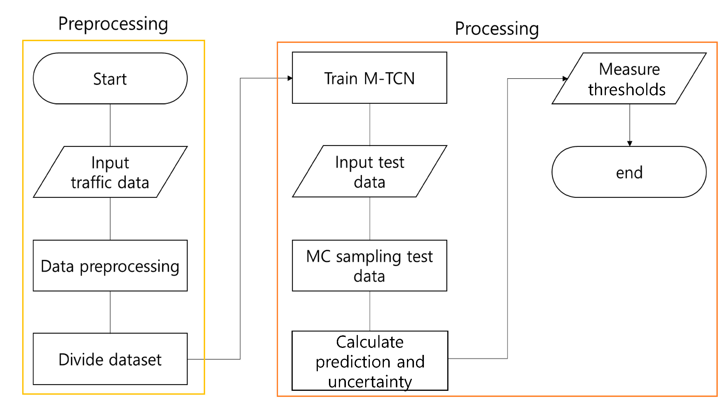
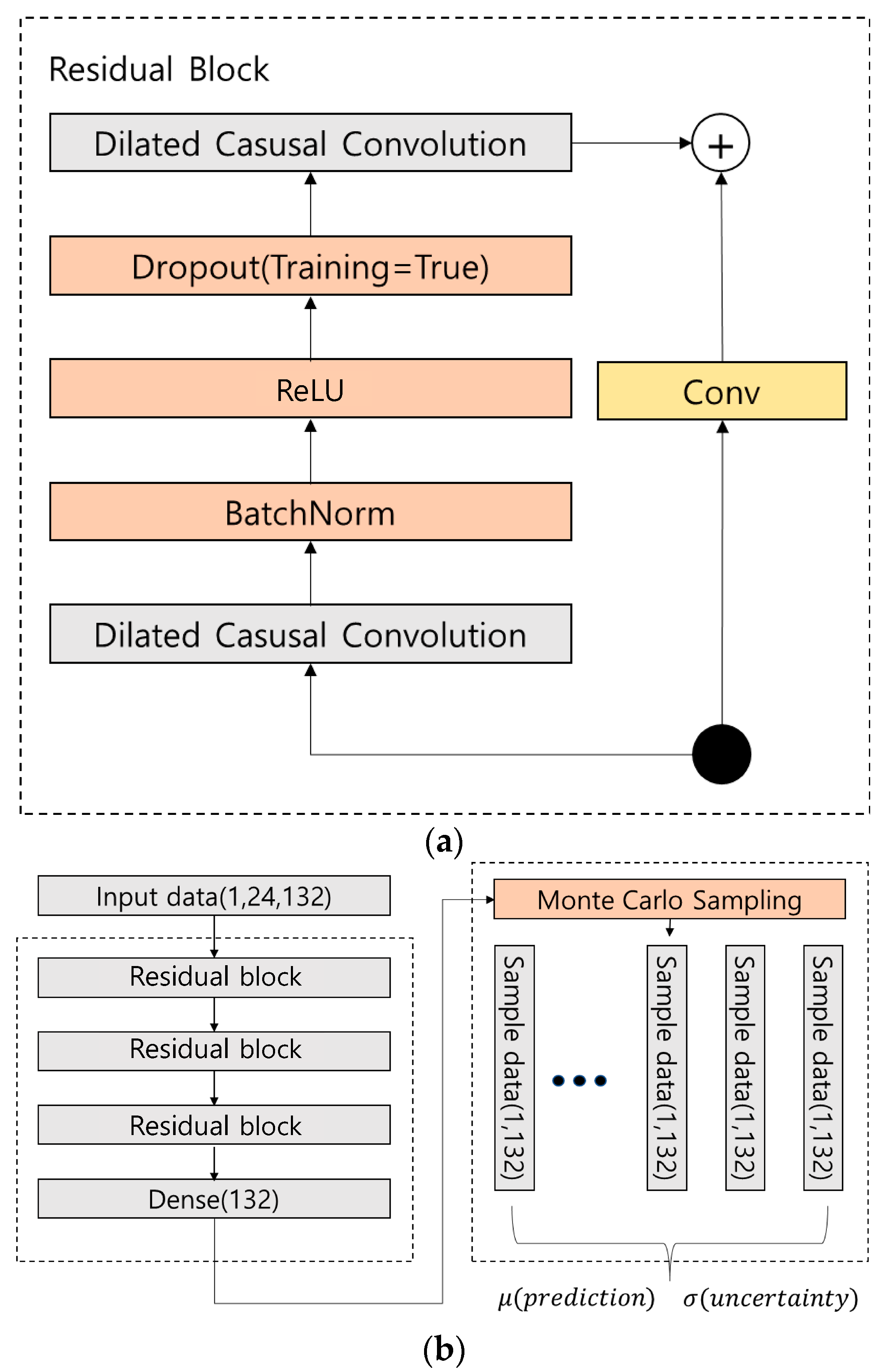
This study reflects the spatiotemporal characteristics of traffic through temporal convolutional networks (TCNs) reflecting the spatiotemporal characteristics, showing better performance than existing time series, deep learning models, LSTM and GRU, and spatial CNN models. In addition, the uncertainty predicted through Monte Carlo dropout can express the reliability of the predicted traffic value, which will enable decision-making support for real-time predictions. Therefore, the Monte Carlo dropout TCN (M-TCN) is proposed, which combines the Monte Carlo dropout (MCDO) and the TCN to express both the predicted values for multiple traffic measurement points in Seoul and the uncertainty of the prediction value. The M-TCN uses the TCN to predict multiple points by considering complex temporal factors and samples, using the MCDO to extract the uncertainty of each point prediction value and confirm the reliability of the model prediction value.
Second, this study proposes a benchmark that can help in decision making through the correlation between uncertainty and error. Through this, it is possible to grasp the predicted value and the degree of uncertainty for multiple points, and make safer and more reliable decisions by reflecting them in the decision-making process.
To solve the above-mentioned problems, this study proposes a new traffic forecasting model, the M-TCN, to check the uncertainty in traffic forecasting. The contributions from this study are as follows:
- (1)
In this study, the MCDO was applied to the TCN models to effectively predict the traffic flow. Through this, it is possible to express the uncertainty of the model that cannot be expressed in the existing traffic model; thus, it is effective not only in predicting traffic, but also in various other places.
- (2)
In this study, the effect of the model’s uncertainty on the error was confirmed, and a normal distribution was used to present a benchmark for the uncertainty value.
- (3)
In this study, the MCDO was applied to various traffic prediction models, and the results were compared to identify differences in the resulting values and to propose an appropriate uncertainty estimation model for traffic flow prediction.
3. Experiments
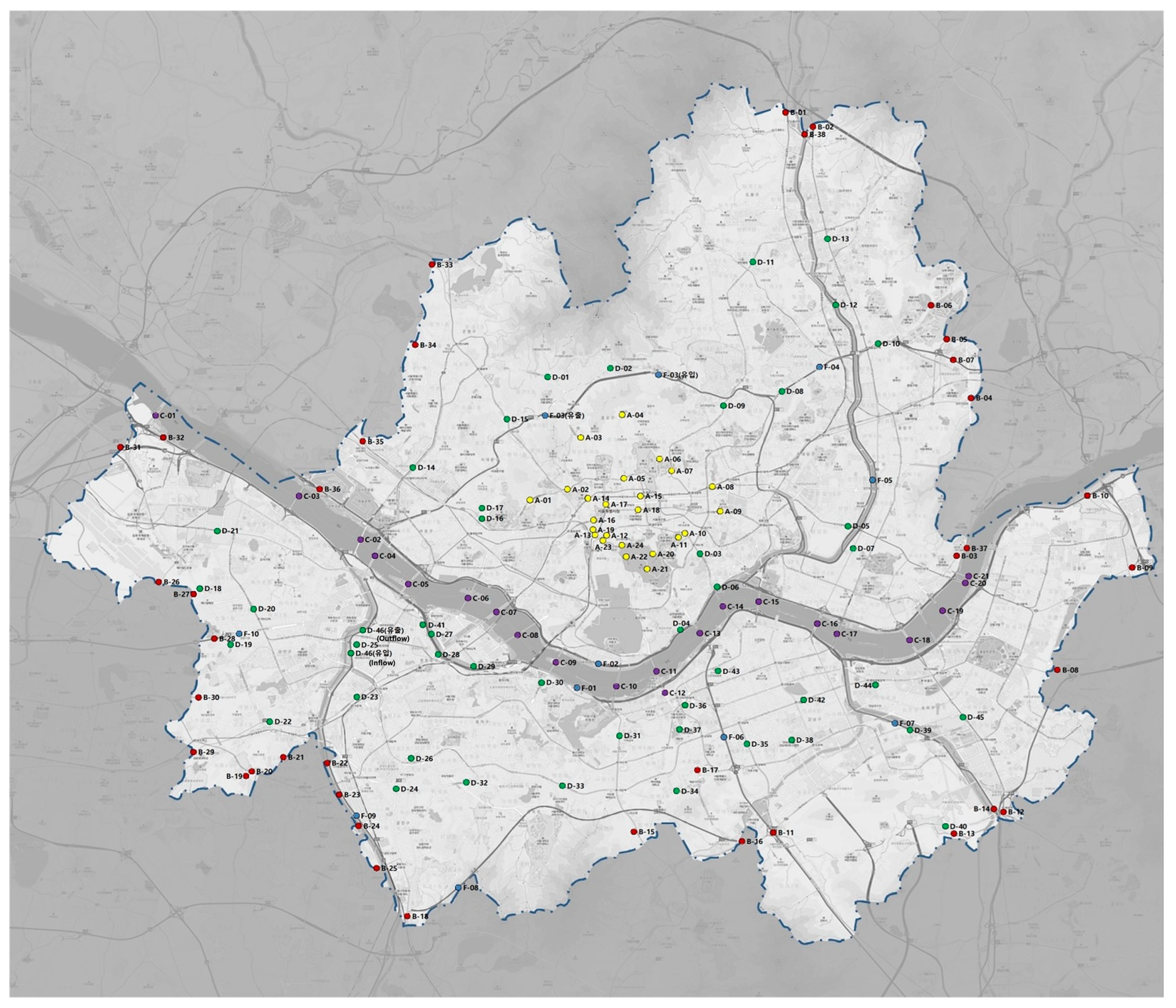
The data used in this study were traffic flow data from Seoul, the capital of Korea, from 1 January 2014 to 30 November 2018, provided by the Seoul traffic information system. The traffic flow dataset for Seoul is described as
Table 1 below. The major highways and urban highways were divided into 132 nodes, and the number of vehicles passing through them per hour was measured. Loop, image, and geomagnetic detectors were used for the measurement.
As shown in
Figure 4, the data were collected from 132 traffic measurement nodes in Seoul, which provided only single traffic data on an hourly basis. The data had a total of 5,729,640 observations, with an average of 39.89 and a standard deviation of 19.58. A total of 23,864 values were missing, accounting for approximately 0.5% of the total. For the missing values, the corresponding values were interpolated using a linear interpolation technique. The interpolated data were divided into train, validation, and test data at a ratio of 6:2:2. The training data were used to teach the model, the validation data to verify the model, and the test data to predict the traffic and evaluate its performance.
In this study, a traffic flow prediction model using the MCDO, which reflects the time series features of the traffic and can estimate the uncertainty, was proposed. The experiment was conducted by applying a timestep of lag 1,12,24 and 6,12,24 to check and compare the short- and long-term prediction performance of the models, with and without the MCDO. Based on previous studies, two models, the LSTM and GRU, were used to predict traffic flow and compare the uncertainty patterns exhibited when models other than those with the MCDO were applied. The timestep and lag were calculated in the same environment as in the above experiment. After the learning stage was completed, Monte Carlo sampling was performed 500 times. In this experiment, four Titan RTX graphics processing units (GPUs) were used, and a total of 850 learning epochs were conducted.
The MCDO was combined in three models that are frequently used in traffic management. For the 6,12,24 timestep and 1,12,24 lag, the result values are summarized as (a), (b), and (c) in
Table 2. (a) The RMSE of the nine result values obtained by applying the MCDO to the TCN was at least 4.68, or a maximum of 6.51, with an average RMSE value of 5.77, and the uncertainty was at least 0.15, or a maximum of 2.42, with an average of 1.21. (b) When the MCDO was applied to the LSTM, the RMSE was at least 4.76, or a maximum of 8.07, with an average RMSE value of 6.51, and the uncertainty was at least 1.94, or a maximum of 3.35, with an average of 2.77. (c) In the case of the CNN, when the MCDO was applied, the RMSE was at least 6.37, or a maximum of 9.03, with an average value of 7.42, and the uncertainty was at least 6.29, or a maximum of 7.33, with an average of 6.82. Overall, the larger the RMSE of the model, the greater the tendency for uncertainty to appear. To verify this in detail, the relationship between the error for the entire test data, as well as the predicted uncertainty must be understood.
The cases with and without the MCDO have the same neural network structure, and the only difference occurs depending on whether dropout is also applied in the test phase. For the dropout model, 500 samples were sampled, and their average was set as the predicted value. According to
Table 3, the short- and long-term prediction performance of the model show a difference of approximately 1% in the RMSE for Lag1, and there is both high and low performance when the MCDO is used. In addition, the difference according to the change in the timestep and lag is approximately 2% and, as in the above case, there is no one-sided performance difference according to the model. It was confirmed that even if the MCDO is applied in the traffic flow prediction model, uncertainty can be exhibited without significantly impairing the performance.
As shown in
Table 3, the models without and with the MCDO show a difference in the performance of approximately 2%; however, there is a difference in the amount of information expressed.
Figure 5 shows a graph of the 116th point for both models; the RMSE is 2.49 without the MCDO and 2.51 with the MCDO. (a) Without the MCDO, only the information about the predicted and actual values is shown, whereas (b) with the MCDO 99% of the uncertainty is provided using Monte Carlo sampling. The larger the corresponding interval, the more difficult it is for the model to trust the current value. The uncertainty is shown in
Figure 6.
Figure 6 shows an enlarged graph of the 175–200 time interval in
Figure 5b, which shows large uncertainties and errors. From 195 to 200 h, the RMSE was 4.27, 71% larger than the RMSE without the MCDO and 70% larger than that with the MCDO. The uncertainty calculated in this section is 2.3 times larger than the average in the other section and contains information indicating that the prediction is less reliable. When using the actual model, if only the performance through the evaluation index for the existing model is considered because the actual value is unknown, the value shows more than 70% variation from the actual value when making decisions.
In addition,
Figure 6 shows that the error widened significantly at the inflection point of the box section, and the uncertainty also tended to increase. The uncertainty value in the section showed a difference of 8.8 to 15.7 times, compared to the 30 h time before the section. Based on this, a hypothesis that there may be a correlation between uncertainty and error was established and verified.
To verify the new hypothesis, the mean absolute error (MAE) and mean standard error (MSE) were obtained through prediction and correlation analyses, with uncertainty additionally performed. As a result of the experiment, the MAE had a positive correlation, with an uncertainty of 34.3% and a p-value of 0.003. The MSE had a positive correlation, with an uncertainty of 31.3% and a p-value of 0.000, confirming that the MAE and the MSE had a positive correlation with uncertainty within the set significance level of 0.05. This means that the greater the uncertainty, the higher the probability that the value predicted by the model differs from the actual value.
Based on this experiment, the uncertainty was correlated with the error. In an actual scenario the predicted value can be inferred; however, the actual value is unknown until a corresponding event occurs. Thus, the performance and predicted value of the model must be used in decision making. However, the use of a specific model will allow uncertainty, which involves a positive correlation between the error and difference between the actual and predicted values, to be identified before the actual value, which may help in decision making.
However, to incorporate this into decision making, it is crucial to have a clear understanding of the level of uncertainty. To simplify decision making, it was imperative to ascertain whether the uncertainty approximated a normal distribution. Hence, the Kolmogorov–Smirnov test was performed. The outcome of this test indicated a test statistic of 0.365 and a p-value of 0.001, confirming that the distribution of uncertainty, with a 99% confidence level, adhered to a normal distribution.
For additional tests, the skewness and kurtosis of uncertainty for a total of 8592 h were analyzed for 132 points. As a result of the analysis, the skewness was 1.53 and the kurtosis was 5.66. Uncertainty follows a normal distribution because the criterion for skewness does not exceed an absolute value of 3, and kurtosis does not exceed an absolute value of 8–10. Based on the test, the reference point according to the magnitude of the uncertainty can be presented through the mean and standard deviation of the uncertainty. Based on the average of the uncertainties, the values of the first standard deviation range were set to be normal uncertainty, low and high for ±2 standard deviations, and very low and very high for ±3 standard deviations, which were determined as outliers. Therefore, it is possible to determine the reliability of the predicted values and use them as indicators to reflect uncertainty in decision making.
5. Conclusions
In this study, the M-TCN model is proposed to estimate the predicted values of traffic flow measurement and the uncertainty of the predicted values in traffic flow prediction. The M-TCN is a combination of the MCDO and the TCN, which is slightly different from the existing model. The experiment conducted in this study was divided into three stages, and the results were as follows. First, even if the MCDO is applied to a traffic model, it does not necessarily degrade the performance of the existing model. For instance, cases of increased performance have also been recorded. Second, a correlation analysis between the error and uncertainty was conducted based on the results obtained by applying the MCDO to the comparison group model and analyzing the uncertainty and RMSE. Consequently, a positive correlation between error and uncertainty was confirmed. Finally, a normality test for uncertainty was conducted to present a benchmark for uncertainty, so that it can be used in decision making. As a result of the test, it was found that uncertainty followed a normal distribution, and a benchmark was set for each standard deviation from ±1 to 3, indicating that uncertainty could be used for decision making. Based on the above results, this study has the following implications.
First, implementing the MCDO does not necessarily degrade the performance of the existing M-TCN model. According to the study results, there was no significant difference in the performance between the models with and without the MCDO and, in some cases, the performance increased. As shown in
Table 3, the prediction performance of the model shows a difference of approximately 1% in the RMSE with Lag1, and the performance varies when the MCDO is implemented. This suggests that uncertainty can be inferred by adjusting only part of the existing AI model, without compromising its overall performance. Such uncertainty can be crucial in scenarios where the reliability of real-time predictions is paramount, as it indicates the trustworthiness of the model beyond simply providing an outcome.
Second, numerous studies have emphasized the importance of considering uncertainty during the decision-making process and post-prediction. There is a correlation between the error and the uncertainty value, signifying the difference between the predicted and actual values of the model. It was verified how the uncertainty derived from the M-TCN model correlates with the actual outcome, allowing its incorporation into the decision-making phase. In real-world scenarios, the immediate acquisition of the actual value is not always feasible; hence, the error in the predicted value remains undetermined. However, experiments have confirmed a positive correlation between uncertainty and error. This suggests that the reliability of the predicted value can be ascertained even when the actual data are not yet available. Decisions can be based on predicted values with high certainty. If the predicted reliability is low, decisions should be approached with caution, considering various possible outcomes, without placing undue trust in the predicted value.
Finally, to incorporate traffic flow uncertainty into the decision-making processes, reference points were introduced to determine the acceptable level of uncertainty for decision makers. Although predicting uncertainty is essential for practical applications, establishing standards for the ideal response based on the magnitude of the predicted uncertainty is equally critical. This study verified that uncertainty adheres to a normal distribution, as determined by a normality test. Subsequently, a benchmark based on standard deviation was proposed.
In conclusion, our study delved into traffic flow dynamics using deep learning, focusing on both point and interval predictions. Although the hourly traffic data is primarily used, the results highlight the potential for more detailed insights in future research. This narrow focus, while intentional for the purpose of this research, hints at the potential benefits of a more expansive analytical approach in future research. By integrating additional data sources, such as real-time feedback from traffic signalling systems and analytics from traffic CCTV systems, future research could achieve a more comprehensive understanding of traffic dynamics.
The shift from point to interval predictions in deep learning is evident, and our research provides valuable insights into this evolving area. Furthermore, our findings have implications beyond the technical aspects. They can influence broader areas, such as the social sciences and traffic policy making. The traffic flow prediction model in this study can be used to establish a traffic demand management plan for sustainable transportation through accurate and reliable prediction, and can contribute to reducing traffic congestion. It will also contribute to improving overall social mobility, reducing energy consumption, and reducing air pollution emissions. As demonstrated in this study, the use of AI can offer new ways to shape traffic policies and decisions. This will lay the groundwork for subsequent research, fostering a more profound comprehension of the nexus between AI, traffic trends, and policy formulation.


