The Dynamic Path Planning of Autonomous Vehicles on Icy and Snowy Roads Based on an Improved Artificial Potential Field

Abstract

The crucial dynamic path planning of autonomous vehicles is achieved via obstacle avoidance path planning technology. The reduction of the tire adhesion coefficient on icy and snowy roads (ISRs) increases the difficulty of autonomous vehicles’ control. In this paper, the driving characteristics of vehicles on ISRs are established, and the artificial potential field function is introduced to avoid collision risk when planning a path. A dynamic path planning algorithm for autonomous vehicles based on the artificial potential field (APF) is established. The adjustment factor is added to the gravitational potential field, and a judgment coefficient is added to the repulsive potential field to improve the artificial potential field function, based on the low adhesion of vehicles on ISRs. Moreover, a path with a continuous curvature is generated to achieve the driving comfort and driving safety of the planned path via trajectory smoothing. By establishing the Carsim/Simulink co-simulation platform, the effectiveness of dynamic path planning for autonomous vehicles under different algorithms and different obstacle models is compared. The results show that the improved APF algorithm has an obvious effect on the smoothness of the path and the reduction of the curvature mutation and can generate a safe and efficient path on icy and snowy roads. The dynamic obstacle avoidance of the improved APF algorithm improves the pre-judgment accuracy of the collision risk assessment of autonomous vehicles and shows the superiority of the improved algorithm.

1. Introduction

The path planning of autonomous vehicles refers to planning an optimal path from the starting point to the target point while completing obstacle avoidance. Accurate path planning is critical to the safe and stable operation of autonomous vehicles. Therefore, many scholars have conducted research on path planning for autonomous vehicles. Currently, such research has mainly focused on path planning algorithms under different constraint conditions. These algorithms establish environmental domain cost functions in road spaces for path planning. Basic methods, such as the A* algorithm [1], Vector Field Histogram (VFH) [2], Artificial Potential Field (APF) [3], and so on, have been used. The curvature of the path planned using the A* algorithm is discontinuous, resulting in significant changes in motion parameters at turning points and making it difficult to apply it reasonably in the field of vehicles. In complex environments that require sensitive obstacle avoidance, the VFH method cannot be used, as it compresses obstacle information into a one-dimensional representation. The basic idea of the APF algorithm is to construct a human potential field in the working environment of vehicle movement. Under the action of the potential field, the vehicle trajectory moves along the gradient direction in which the resultant force field decreases the fastest, making it more suitable for the path planning of vehicle trajectories.

However, due to the two problems of the local minimum and an unreachable target, traditional artificial potential algorithms have limitations. By improving the gravitational and repulsive potential fields, the drawbacks of APF can be avoided. At present, there are many measures to improve the repulsive potential field, including introducing a repulsive field adjustment factor [4] and reconstructing the repulsive field range of obstacles [5,6] and the repulsive field range of road boundaries [7]. Some scholars have introduced dangerous potential fields [8], or velocity-difference potential fields and acceleration-difference potential fields [9], to improve traditional artificial potential algorithms. Some scholars have comprehensively considered the distance adjustment factor, dynamic road repulsion field, velocity repulsion field, and acceleration repulsion field to complete autonomous driving trajectory planning [10]. In addition to improving the potential field function, the APF algorithm can also be integrated with other algorithms. This includes the Rapid Exploration Random Tree (RRT) algorithm [11], A* algorithm [12], complex resistivity method [13], ant colony algorithm [14], and cyclic reinforcement learning algorithm [15]. The fusion algorithm can enable autonomous vehicles to avoid obstacles more safely and achieve the purpose of complementary advantages.

Different smoothing functions can be introduced to address the problem of uneven planned path trajectories obtained using the APF algorithm; for example, using the Sequential Quadratic Programming (SQP) algorithm to solve precise paths that meet safety requirements [16] and introducing the LC algorithm to provide smoother and safer humanoid trajectories [17]. In addition, it is also possible to consider establishing constraints on vehicle dynamics and different types of obstacles [18] and safety distance models in different scenarios [19], as well as providing adaptive motion planning strategies for fuzzy systems [20]. These measures can improve the safety and smoothness of traditional APF path planning by correlating a vehicle’s automatic collision avoidance system with changes in the collision area.

The actual road scene is complex and unpredictable. So, the effectiveness of vehicle path planning algorithms can be verified through different experimental scenarios. Road scenes can be viewed from different perspectives, including different obstacle environments [21], dynamic obstacle environments [22], constant-speed and variable-speed obstacle vehicle environments [23], and different manual-driving vehicle environments [24]. The artificial potential field algorithm can be improved from various perspectives to adapt to different road scenarios. For example, in order to solve the problem of path planning under different velocities and different types of obstacles, Liu et al. (2021) proposed an adaptive path planning system with two fused potential fields [25].

The researchers improved the artificial potential field algorithm from three aspects: potential field function, path smoothing, and obstacle avoidance in different scenarios. The above research has improved the APF algorithm from different perspectives. However, vehicle dynamics and APF potential field functions in special environments, such as ice and snow, need to be redesigned. At the same time, different types of obstacles to vehicles also have a significant impact on the dynamic obstacle avoidance path planning of vehicles. Therefore, this article proposes a dynamic path planning algorithm for autonomous vehicles on ISRs based on an improved APF. This algorithm considers the driving characteristics of vehicles on ISRs, ensuring the applicability of the planned path. Meanwhile, by improving the APF algorithm, curvature continuous paths can be generated, meeting the driving comfort and safety requirements of the planned path. Finally, the proposed method was simulated and validated through Carsim/Simulink to determine the effectiveness and reliability of the algorithm. The flowchart of this article is shown in Figure 1.

The research contents of this paper are as follows: Section 2 introduces the improved algorithm proposed in this paper in detail. Firstly, the principle of the traditional APF algorithm is introduced. According to the influence of the driving characteristics of the vehicle in an ISR environment, the gravitational potential field and the repulsive potential field are improved. Finally, the dynamic processing and trajectory smoothing of the planning path results are carried out, and the dynamic planning path of the autonomous vehicle in an ISR environment, based on the improved artificial potential field algorithm, is obtained. Section 3 introduces the simulation platform for testing the effectiveness of the improved APF algorithm. The comparative experiments of vehicle performance parameters under different algorithms and different models are designed and discussed. Section 4 summarizes the full paper.

2. Methods

2.1. Traditional APF Algorithm

For path planning problems, the entire artificial potential field U in the motion space is the vector superposition of the gravitational potential field (U_att) and the repulsive potential field (U_rep) [26], that is U = U_att + U_rep. The gravitational potential field ensures the vehicle’s global tracking of the target state, while the repulsive potential field ensures the vehicle’s safe avoidance of multiple obstacles. By calculating the direction of the combined force of the gravitational and repulsive potential fields, the path along which the potential function descends is selected to reach the global minimum potential field. According to the definition of a potential field, vehicles always have a tendency to move towards low-potential-energy regions. Therefore, starting from the planning starting point, vehicles use the potential energy difference of the virtual potential field to move, and their movement trajectory is the planning path of the APF algorithm.

2.1.1. Gravitational Potential Field

The gravitational potential field potential energy of a vehicle monotonically increases as its distance from a target increases. In path planning problems, vehicles can be treated as particles, X = (x,y)^T, in a two-dimensional space environment, with their motion space being a two-dimensional space. In traditional APF algorithms, the gravitational potential field (U_att) generated using the target point is generally expressed as:

$$U_{att}\left(X\right)=\frac{1}{2}{k}_{att}\times {\rho }^m\left(X,X_g\right)$$

(1)

In this formula: k_att indicates the positive proportional gain factor of the gravitational potential field; X denotes the position coordinate of the vehicle; X_g represents the position coordinates of the target point; m indicates the gravitational potential field factor—in this paper, m = 2; and $\rho \left(X,X_g\right)=‖X_g-X‖$ represents the relative distance between the vehicle and the target.

The gravitational force generated by the vehicle, F_att, represents the fastest descent direction of the gravitational potential field (U_att), and its expression is as follows:

$$F_{att}\left(X\right)=-\nabla U_{att}\left(X\right)=-k_{att}\cdot \left(X,X_g\right)$$

(2)

2.1.2. Repulsive Potential Field

The repulsive potential field potential energy of a vehicle monotonically decreases as its distance from the obstacle increases. When reaching an obstacle, the repulsive potential energy of the vehicle is infinite, indicating that the repulsive potential field should try to avoid colliding with the obstacle as much as possible. In traditional APF algorithms, the repulsive potential field (U_rep) generated via obstacles can usually be expressed as follows:

$$U_{rep}\left(X\right)=\left\{\begin{array}{cc}\frac{1}{2}{k}_{rep}\left(\frac{1}{\rho (X,X_0)}-\frac{1}{{\rho }_0}\right)& \rho (X,X_0)\le {\rho }_0\\ 0 & \rho (X,X_0)>{\rho }_0\end{array}\right.$$

(3)

In this formula: k_rep indicates the positive proportional gain factor of the repulsive potential field; X₀ represents the position coordinates of obstacles; ${\rho }_0$ represents the maximum influence distance of the obstacle repulsive potential field; and $\rho \left(X,X_g\right)=‖X_g-X‖$ indicates the relative distance between the vehicle and the obstacle.

The repulsive force (F_rep) generated via obstacles represents the fastest descent direction of the repulsive potential field (U_rep), and its expression is as follows:

$$F_{rep}\left(X\right)=\left\{\begin{array}{cc}{k}_{rep}\left(\frac{1}{\rho (X,X_0)}-\frac{1}{{\rho }_0}\right) \frac{1}{{\rho }^2(X,X_0)} \frac{\partial \rho (X,X_0)}{\partial X}& ,\rho (X,X_0)\le {\rho }_0\\ 0 & ,\rho (X,X_0)>{\rho }_0\end{array}\right.$$

(4)

2.1.3. Composite Potential Field

The total potential field function U(X) is the composite potential field that combines two potential fields:

$$U\left(X\right)=U_{att}\left(X\right)+U_{rep}\left(X\right)$$

(5)

Similarly, the resultant force F(X) on the vehicle is the vector resultant force of the gravitational force F_att(X) and the repulsive force F_rep(X), as shown in Figure 2.

$$F(X)=-\nabla U\left(X\right)=F_{att}\left(X\right)+F_{rep}\left(X\right)$$

(6)

Using Formulas (5) and (6), the potential energy and potential field resultant force of each point in the moving space can be calculated. The vehicle moves under the guidance of a synthetic potential field until it reaches the target point. The trajectory of a vehicle is the planned path. According to the potential energy difference of the potential field, the curve with the fastest descent along the potential field function U(X), which is the global optimal path, is selected.

2.2. Driving Characteristics of Vehicles in an ISR Environment and a Modeling Scenario

ISRs have an impact on the longitudinal and lateral driving of vehicles. A longitudinal braking distance model for icy and snowy roads was constructed in terms of longitudinal driving, and a lateral displacement model for icy and snowy roads was constructed in terms of lateral driving. The artificial potential field can be improved using the two indicators of longitudinal braking distance and lateral displacement as limiting conditions.

2.2.1. Longitudinal Braking Distance Model on ISRs

For the longitudinal braking distance model on icy and snowy roads, inspiration was drawn from Macnabb’s tracking and testing of vehicle traction and braking capabilities on winter roads [27]. Based on the test results of different vehicles and tires, taking into account the driving speed and stopping distance of vehicles on icy and snowy roads, the friction coefficient calculation formula is as follows:

$$\mu =\frac{V^2}{254\times d_l}$$

(7)

In this formula, V represents the driving speed (km/h), and d_l indicates the longitudinal braking distance on ISRs (m).

When the friction coefficient in icy and snowy weather is known, the longitudinal braking distance model of the vehicle at the corresponding speed can be obtained according to Formula (8):

$$d_l=\frac{V^2}{254\times \mu }$$

(8)

2.2.2. Lateral Displacement Model of ISRs

When a vehicle is changing lanes, mechanical balance can be used to study the balance problem of the vehicle. By decomposing the force acting on the vehicle along the lateral and vertical (x-axis, y-axis) of the vehicle body, the following equation can be obtained based on the force balance:

$$m{a}_y\cos \beta =F_{fi}+F_{fo}+mg\sin \beta$$

(9)

$$m{a}_y\cos \beta =F_{fi}+F_{fo}+mg\sin \beta$$

(10)

In this formula: m represents the vehicle mass (kg); α_y represents the lateral acceleration of vehicles on ISRs (m/s²); g indicates the gravitational acceleration (m/s²); β represents the road slope; F_fi and F_fo represent the friction force of vehicles on ISRs (N); and N_i and N₀ indicated the supporting force of the road surface on the vehicle (N).When the vehicle is about to slip, the maximum lateral friction force of the tires is equal to the adhesion between the wheels and the road surface:

$$(N_i+N_o)\mu =F_{fi}+F_{fo}$$

(11)

In this formula, μ represents the road adhesion coefficient on ISRs.

The lateral acceleration of the vehicle under the critical state of sideslip can be obtained by combining Formulas (9)–(11), as follows:

$$a_{yc}=\frac{\mu g\cos \beta +g\sin \beta }{\cos \beta -\mu \sin \beta }$$

(12)

In this formula, α_yc represents the lateral acceleration of the vehicle in a critical state (m/s²).

According to the “Technical Standards for Highway Engineering” [28], the recommended superelevation values for curved road sections are provided, and sin β can be converted to be approximately equal to i, and cos β to be approximately equal to 1. Therefore, the formula can be simplified as follows:

$$a_{yc}=\frac{\mu g+ig}{1-\mu i}$$

(13)

In this formula, i indicates the superelevation value of curved road sections.

The lateral displacement value is related to the lateral acceleration and driving speed, and the relationship formula is as follows:

$$d_c=\frac{V_t^2-V_0^2}{2a_{yc}}=\frac{(V_t^2-V_0^2)\cdot (1-\mu i)}{2(\mu g-ig)}$$

(14)

In this formula: V₀ represents the driving speed before acceleration (km/h); V_t represents the driving speed after acceleration (km/h); and d_c represents the lateral displacement value on an ISR surface (m).

2.2.3. Modeling Scenario Description

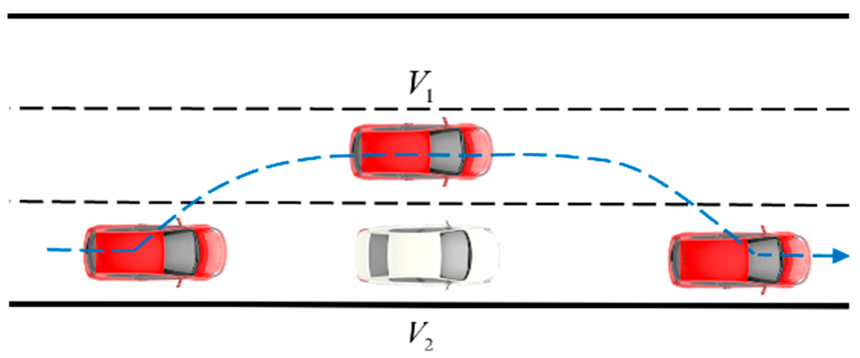
When two vehicles are in the same lane and the obstacle vehicles in front of this lane are moving slowly, it is necessary to change lanes or overtake to avoid traffic accidents such as scratches and collisions between the two vehicles. The target vehicle generally needs to turn to avoid obstacles, as the speed situation is complex and variable. Therefore, this article only discusses the situation in which the obstacle vehicle ahead is traveling at a uniform speed and the target vehicle is traveling at a uniform longitudinal speed in a straight-road driving scenario. And the target vehicle’s speed is greater than the obstacle vehicle ahead, and there are no other vehicles or obstacles around the two vehicles. When this scenario is taken as the research content, the effectiveness of dynamic path planning for an autonomous vehicle was verified under two working conditions for static obstacle vehicles and dynamic obstacle vehicles. The straight-lane scenario is shown in Figure 3, in which the red vehicle is the target vehicle, with a longitudinal speed V₁ of 8 m/s, and the white vehicle is the obstacle vehicle, with a speed V₂ of 10 m/s.

2.3. Improved APF Algorithm in an ISR Environment

Due to the low friction coefficient of ISRs, the driving dynamics characteristics of a vehicle will change significantly. Based on the driving characteristics of vehicles on ISRs, it can be concluded that changes in the braking distance and control direction of vehicles will have an impact on traditional APF algorithms. The specific analysis is as follows.

2.3.1. The Influence on the Gravitational Potential Field

Vehicles should reserve sufficient braking and steering space on ISRs, which can increase the adjustment factor (α_att) on the original gravitational potential field (U_att). The ISR conditions will affect α_att. The lower the friction coefficient on ISRs, the larger α_att, and the greater U_att, which is the line connecting the vehicle and the target position that points towards the target point. The regulatory factor (α_att) and the gravitational potential field (U_att) are represented as follows:

$${\alpha }_{att}=\frac{\sqrt{d_l^2+d_c^2}}{\sqrt{D_l^2+D_c^2}}$$

(15)

$$U_{att}^{*}\left(X\right)=\frac{1}{2}{\alpha }_{att}\cdot k_{att}\cdot {\rho }^2\left(X,X_g\right)$$

(16)

In this formula, D_l represents the longitudinal braking distance on a normal road surface (m) and D_c represents the lateral displacement value on a normal road surface (m).

2.3.2. Influence on Repulsive Potential Field

The repulsive potential field is generated using several obstacles in the environment, and its shape resembles a “high ground” in the potential field. A judgment coefficient (α_rep) is added to the original repulsive potential field function (U_rep). The judgment coefficient (α_rep) and the repulsive potential field function (U_rep) are expressed as follows:

$${\alpha }_{rep}=\sqrt{d_l^2+d_c^2}-\sqrt{D_l^2+D_c^2}$$

(17)

$$U_{{}_{rep}}^{*}\left(X\right)=\left\{\begin{array}{cc}\frac{1}{2}{k}_{rep}\left(\frac{1}{\rho (X,X_0)}-\frac{1}{{\rho }_0}\right)& \rho (X,X_0)\le {\rho }_0+{\alpha }_{rep}\\ 0 & \rho (X,X_0)>{\rho }_0+{\alpha }_{rep}\end{array}\right.$$

(18)

In Formula (18), the value of α_rep is influenced by the iciness and snowiness of the road surface. The lower the friction coefficient of the ISR surface, the larger the value of α_rep and the greater the space reserved for judging conditions, thereby avoiding collisions with obstacles.

2.3.3. The Impact on the Resultant Potential Field

The combined potential field U*(X) is obtained by overlaying the gravitational potential field ($U_{att}^{*}$) and the repulsive potential field ($U_{rep}^{*}$) on the icy and snowy road surface.

$$U^{*}\left(X\right)=U_{att}^{*}\left(X\right)+U_{rep}^{*}\left(X\right)$$

(19)

As shown in Figure 4, for the improved APF algorithm that was constructed, a one-way, three-lane-road-environment APF was drawn. The potential field at the centerline of each lane is the lowest, so it can guide vehicles to travel in the middle of the lane. In order to prevent vehicles from exiting the lane, the potential field at the road boundary is the highest, and it grows faster as it approaches the boundary. The potential field at the lane boundary is between the centerline of the lane and the outer boundary, meaning that vehicles can pass through the lane boundary when changing lanes but cannot drive on the lane boundary for a long time.

2.4. Path Smoothing and Dynamic Planning

Curve fitting was performed on the discrete local optimal reference path points generated via the APF to ensure the smoothness and continuity of the autonomous driving path. Due to the simple structure, low computational complexity, and continuous curves of polynomials, this article used a fifth-degree polynomial to fit the lateral displacement and deflection angle of vehicles. The specific formula is as follows:

$$\left\{\begin{array}{c}{Y}_{ref}=a_5{X}^5+a_4{X}^4+a_3{X}^3+a_2{X}^2+a_1{X}^1+a_0\\ {\phi }_{ref}=b_5{X}^5+b_4{X}^4+b_3{X}^3+b_2{X}^2+b_1{X}^1+b_0\end{array}\right.$$

(20)

In the formula: a and b are both undetermined coefficients, $a=(a_5,a_4,a_3,a_2,a_1,a_0)$; $b=(b_5,b_4,b_3,b_2,b_1,b_0)$.

When the obstacle vehicle and the target vehicle move together, the planned path of each sampling point is a local target path. The real-time vehicle location and road environment information are collected by setting a fixed sampling time interval. Each time, the vehicle path is re-planned and updated to achieve the dynamic planning of autonomous vehicle paths. Figure 5 is a schematic diagram of the dynamic path planning when the target vehicle overtakes.

2.5. The Process of APF Algorithm in an ISR Environment

The process of the APF algorithm under ISR environment conditions is as follows:

Step 1: Load the drawn road map;

Step 2: Initialize vehicle-related parameters, including the starting point, target point, initial direction, vehicle size, maximum speed and acceleration, repulsion influence range, safety distance range, repulsion force proportion factor, etc.;

Step 3: Before path planning, first check the legitimacy of the starting point and target point. If the location is set in an obstacle, it will definitely not be able to reach that state, and the planning is canceled;

Step 4: After confirming that the starting state and target state are both legal, detect whether the target has been reached each time. If the target has been reached, the planning will end. If the target has not been reached, continue with the next step of planning;

Step 5: Substitute the mathematical model of the improved APF algorithm to calculate the vector size and direction of the repulsion force based on the number of obstacles, distance, angle, etc. Also, calculate the vector size and direction of gravity. Finally, the direction and magnitude of the entire synthetic force are obtained;

Step 6: Calculate the vehicle’s next forward direction, forward speed, forward distance, etc., based on the magnitude and direction of the synthesized force, and drive the vehicle forward;

Step 7: Detect whether the target point has been reached. If not, continue to plan according to the process until the target point is reached.

3. Simulation and Result

3.1. Simulation Platform Construction

Using the joint simulation platform of MATLAB 2020a and Carsim 2019, the effectiveness of the improved artificial potential field algorithm for dynamic path planning on ISRs was simulated and verified. Simulink was used for the dynamic path planning and trajectory tracking control of vehicles. The road environment and output of the operating parameters of the target vehicle were provided using Carsim. The joint simulation process is shown in Figure 6. Based on dynamic road environment information and the improved artificial potential field algorithm, global planning paths for autonomous vehicles on ISRs were generated using MATLAB. The planned path was input into the path planning module and the track tracking module in Simlink. The output vehicle variables, such as the front wheel angle, which act on the vehicle dynamics model in Carsim, were output as a real-time vehicle status. The simulation environment was MATLAB 2021a, and the hardware platform was Win11+AMD R7 5800 H CPU@3.20 GHz+16 GB RAM. The simulation parameters of the lane and target vehicle are shown in

Table 1. Simulation parameters.

Symbols	Name	Value
wroad	Lane width	3.50 m
lroad	Lane length	100 m
nroad	Lane number	2
wcar	Vehicle lateral length	1.80 m
lcar	Vehicle longitudinal length	4.70 m

.

Different types of icy and snowy road surfaces have different road adhesion coefficients, and the trajectory parameters of vehicles changing lanes on ISRs with different adhesion coefficients are also different.

Table 2. The attachment coefficient of different snowy and icy roads.

Icy and Snowy Road Surface	Coefficient of Adhesion
Ice	0.05–0.1
Compacted snow surface	0.1–0.2
Ordinary snow surface	0.2–0.25
Melting snow surface	0.25–0.3

shows the range variation of the adhesion coefficient for different icy and snowy road surfaces.

According to the actual situation of urban road vehicles, taking the urban two-lane road as an example, the functional verification of the improved APF algorithm in the dynamic environment was carried out. This scenario assumed that the vehicle was traveling on two lanes, and the target lane of the main vehicle was determined to be the left lane, according to the lane change decision. The yellow target vehicle was run at a uniform speed of 10 m/s, the starting point coordinate was (0, 1.75), and the end point coordinate was (100.75). There were two black obstacle vehicles with a speed of 5 m/s in front of the target lane. The initial coordinates of the two obstacle vehicles were (20, 1.75) and (30, −1.75), respectively. The road adhesion coefficient adopted the critical value of the adhesion coefficient of the ordinary snow surface in Table 2, and the value was 0.25. Because the higher the sampling frequency, the better the path result, the environment perception update time of the autonomous vehicle was set to 0.1 s.

The simulation results obtained through MATLAB are shown in Figure 7. Figure 7 shows the trajectory planning process of a straight two-lane lane change with two dynamic obstacles. In Figure 7, the horizontal axis represents the length of the lane (l_road), and the vertical axis represents the width of the lane (w_road). The red solid line is the final driving path, the white car is the target vehicle, the yellow car is the current location of the target vehicle, and the gray car is the obstacle vehicle. The vehicle trajectories when the state of the target vehicle changes were extracted for analysis. Starting from the starting point of the main vehicle, the autonomous vehicle sensor transmitted the surrounding environment state data to the improved APF algorithm, including the starting and ending position obtained in the global path planning stage, the position and speed of the surrounding vehicle, the road adhesion coefficient, and other information. At the starting moment, the target vehicle was barrier-free. In addition to the repulsive potential field at the road boundary, the target vehicle was only affected by the gravitational potential field at the end point, so the target vehicle was run in a straight line. When an obstacle vehicle is encountered, the target vehicle is affected by the repulsive potential field, the resultant potential field plans a new path trajectory, and path smoothing is performed using a fifth-order polynomial. Under the action of the resultant force potential field, the target vehicle completed the lane change. Due to the existence of obstacle vehicles, the target vehicle could not immediately return to the original lane; that is, it still needed to maintain the current lane. When the target vehicle overtook the obstacle vehicle, due to the influence of the resultant force potential field, the vehicle would return to the original lane and complete the entire overtaking process.

It can be seen that the improved artificial potential field algorithm can complete obstacle avoidance path planning with moving obstacles effectively. The planned path was closer to the actual path of the vehicle, and the planned path was smoother, indicating that the improved obstacle model can guide vehicles’ lane-changing behavior.

3.2. Analysis of the Dynamic Obstacle Avoidance Effectiveness of the Improved APF Algorithm

In order to verify the effectiveness and reliability of the improved APF algorithm for dynamic obstacle avoidance on ISRs, the vehicle dynamics parameters were analyzed under three obstacle avoidance scenarios: the static obstacle avoidance of the traditional APF algorithm (SOA-APF), the dynamic obstacle avoidance of the traditional APF algorithm (DOA-APF), and the dynamic obstacle avoidance of the improved APF algorithm (DOA-IAPF). The applicability of the improved APF algorithm when the vehicle speed was 8 m/s and 10 m/s was compared. Simultaneously, a comparative obstacle avoidance algorithm, the dynamic obstacle avoidance of the traditional RRT algorithm (DOA-RRT), was added. The parameters of each obstacle avoidance scenario are shown in

Table 3. Parameters of different obstacle avoidance scenarios.

Position	DOA-RRT	SOA-APF	DOA-APF	DOA-IAPF
Start point	(0, 1.75)	(0, −1.75)	(0, −1.75)	(0, 1.75)
End point	(100, 1.75)	(100, 1.75)	(100, 1.75)	(100, 1.75)
Obstacle 1	(20, 1.75)	(25, −3)	(15, 1.75)	(20, 1.75)
Obstacle 2	(30, −1.75)	(50, 3)	(45, −2.5)	(30, −1.75)
Obstacle 3	/	(75, −3)	/	/
Obstacle status	Motion	Stillness	Motion	Motion

.

With a target vehicle speed was 8 m/s, the simulation results of the yaw angle, yaw rate, and front wheel angle under different obstacle avoidance scenarios are shown in Figure 8. SOA-APF achieved the worst performance, with maximum yaw angles of −19.95 dge and 17.33 dge for two lane changes, respectively. The yaw angle fluctuated greatly, and the trajectory was not smooth, which caused a sudden change phenomenon from 10 s to 12 s. DOA-APF performed relatively well, but the fluctuation amplitude was still high, with a maximum yaw angle of 14.72 dge. The overall fluctuation of DOA-RRT was relatively low. But when the target vehicle overtook, there was a sudden change in the front wheel angle and yaw intersection of the target vehicle. At the same time, the path planned using DOA-RRT did not achieve the constraint of a safe vehicle distance. DOA-IAPF achieved the best performance, with a maximum yaw angle of −9.30 dge for both lane changes. Compared to the other three methods, the yaw angle fluctuation of DOA-IAPF was low, and there was no sudden change phenomenon. Similar to the trend in yaw angle variation, the limit values and fluctuation of the yaw rate and front wheel angle obtained using DOA-IAPF were relatively low and superior to the other three methods. The effectiveness of the improved APF algorithm for dynamic obstacles was proven.

When the target vehicle speed is 10 m/s, the yaw angle, yaw rate, and front wheel angle are shown in Figure 9. It can be found that DOA-IAPF is still superior to the other three methods at different speeds. However, when the target vehicle speed is 10 m/s, the angle change per unit time becomes larger. Therefore, the variation amplitude and peak value of various parameters are all less than the vehicle speed of 8 m/s.

3.3. Analysis of Obstacle Avoidance Effectiveness for Different Obstacle Vehicle Types

In order to verify the adaptability of the algorithm in different scenarios and compare the impact of different obstacle vehicle types on DOA-IAPF, the vehicle dynamic parameters when overtaking under different obstacle vehicle types were analyzed. This paper divided obstacle vehicles into three types of vehicles, with the length and width of the vehicles taking the average of the current vehicle classification standards. The specific parameter values for obstacle vehicles of different models are shown in

Table 4. Obstacle vehicle parameters.

Vehicle Type	Longitudinal Length/m	Lateral Length/m
Large vehicles	7.18	2.55
Medium vehicles	6.00	2.15
Small vehicles	4.70	1.80

.

With a target vehicle speed was 8 m/s, the simulation results of the yaw angle, yaw rate, and front wheel angle for different obstacle vehicle types are shown in Figure 10. Evading large-obstacle vehicles started from the 5.2nd second and ended at the 13.5th second, lasting for 8.3 s, for which the maximum yaw angle was 3.60 rad. Evading medium-obstacle vehicles started from the 8.9th second and ended at the 15.1st second, lasting for 6.2 s, for which the maximum yaw angle was 6.00 rad. Evading small-obstacle vehicles started from the 10.0th second and ended at the 15.4th second, lasting for 5.4 s, for which the maximum yaw angle was 7.65 rad. Due to the large volume of large vehicles, the generated repulsive potential field was large, which caused the target vehicle to change lanes ahead of time and resulted in a long lane-changing time and small changes in the yaw angle. Therefore, the yaw rate and front wheel angle of large vehicles are also lower compared to other models.

4. Conclusions

In this paper, we proposed an improved artificial potential field algorithm to improve the efficiency and accuracy of autonomous vehicle path planning in an ISR environment. The reliability of the model was verified by comparing the vehicle planning trajectories at different speeds and under different obstacle avoidance conditions.

• Considering the driving characteristics of vehicles on ISRs, the gravitational field and repulsive field models of the traditional APF algorithm were improved by adding adjustment factors and judgment coefficients. The improved APF algorithm proposed in this paper can plan a smooth lane change and overtaking path, effectively avoid obstacle vehicles, and guide autonomous vehicles to drive safely and stably.
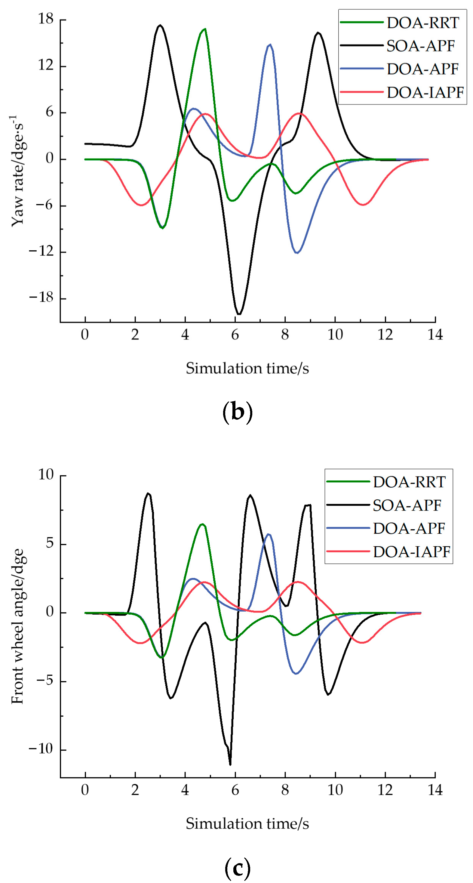
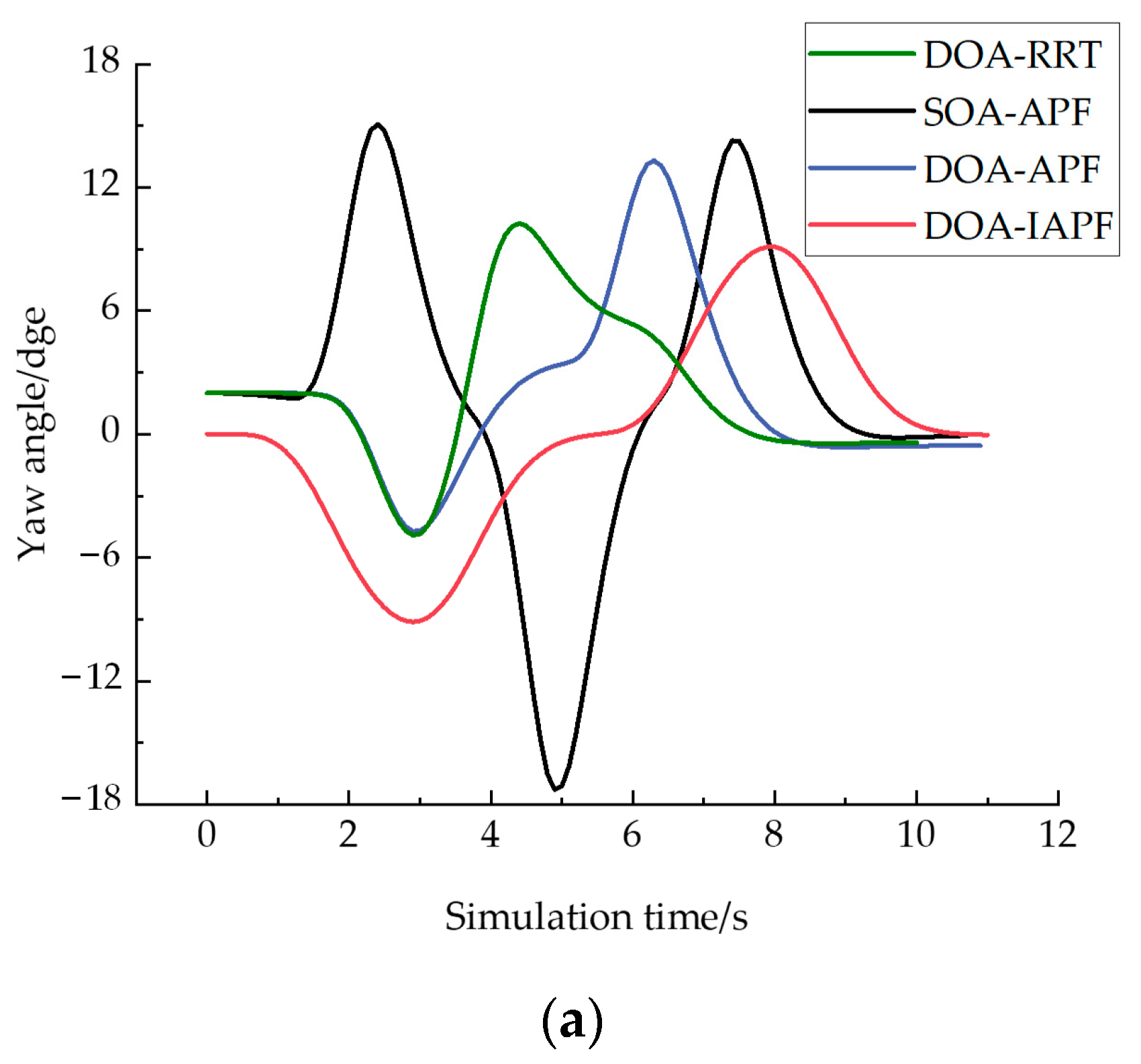
• The effectiveness of the improved APF algorithm was verified by comparing it with the traditional APF algorithm under dynamic planning path and vehicle conditions. The results show that, compared with the static obstacle avoidance and dynamic obstacle avoidance of the traditional APF algorithm, the trajectory of the dynamic obstacle avoidance path planned using the improved APF algorithm was smoother, and there was no mutation.
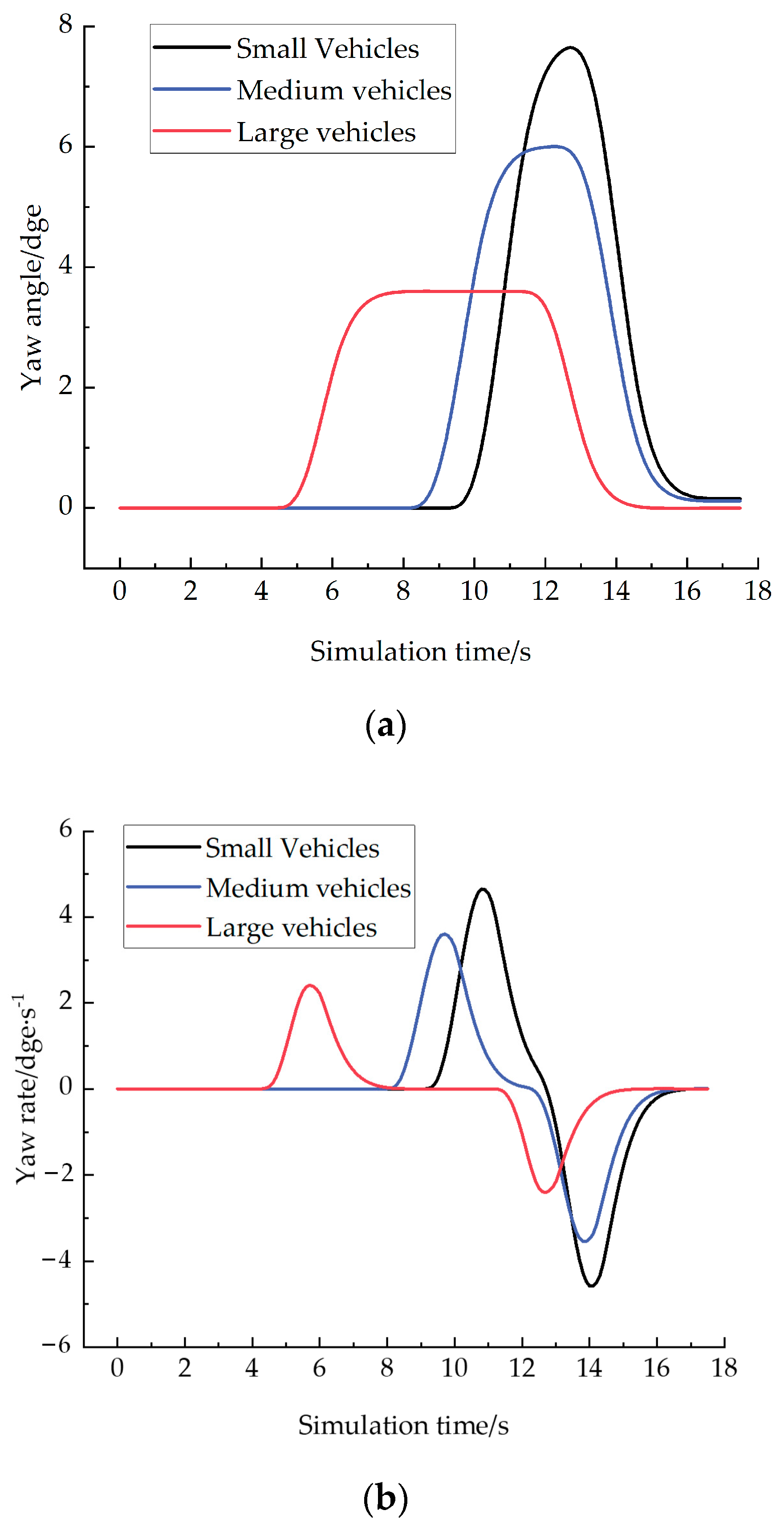
• The obstacle avoidance accuracy and efficiency of autonomous vehicles for different obstacle models were analyzed. The results show that the improved APF algorithm can generate different planning paths for different types of obstacle vehicles and can safely and effectively guide an autonomous vehicle to complete obstacle avoidance and lane changes.

Future work will consider more complex traffic scenarios, as well as different driving styles for decision-making and motion planning. For example, the article’s assumption was that the motion state of the obstacle vehicle remained unchanged. We did not consider a situation in which a car was driving around a bend and the movement status of obstacle vehicles changed randomly. For more complex driving environments, such as multiple lanes, unsignalized intersections, and roundabouts, the reliability of the algorithm needs to be verified by considering different driving environments. At the same time, the speed required in this paper was manually preset. If the required speed can be determined according to different driving conditions and driving styles, the APF algorithm can be further improved. In addition, it is necessary to test the motion planning performance of the improved APF algorithm in a real scene through a real vehicle platform, which will be the focus of future research.

References

1. Yershov, D.S.; LaValle, S.M. Simplicial Dijkstra and A* Algorithms for Optimal Feedback Planning. In Proceedings of the 2011 IEEE/RSJ International Conference on Intelligent Robots and Systems, San Francisco, CA, USA, 25–30 September 2011; pp. 3862–3867. [Google Scholar]
2. Borenstein, J.; Koren, Y. The Vector Field Histogram-Fast Obstacle Avoidance for Mobile Robots. IEEE Trans. Robot. Autom. 1991, 7, 278–288. [Google Scholar] [CrossRef]
3. Barraquand, J.; Langlois, B.; Latombe, J.-C. Numerical Potential Field Techniques for Robot Path Planning. IEEE Trans. Syst. Man Cybern. 1992, 22, 224–241. [Google Scholar] [CrossRef]
4. Wu, H.; Zhang, Y.; Huang, L.; Zhang, J.; Luan, Z.; Zhao, W.; Chen, F. Research on Vehicle Obstacle Avoidance Path Planning Based on APF-PSO. Proc. Inst. Mech. Eng. Part D-J. Automob. Eng. 2023, 237, 1391–1405. [Google Scholar] [CrossRef]
5. Wang, P.; Gao, S.; Li, L.; Sun, B.; Cheng, S. Obstacle Avoidance Path Planning Design for Autonomous Driving Vehicles Based on an Improved Artificial Potential Field Algorithm. Energies 2019, 12, 2342. [Google Scholar] [CrossRef]
6. Rasekhipour, Y.; Khajepour, A.; Chen, S.-K.; Litkouhi, B. A Potential Field-Based Model Predictive Path-Planning Controller for Autonomous Road Vehicles. IEEE Trans. Intell. Transp. Syst. 2017, 18, 1255–1267. [Google Scholar] [CrossRef]
7. Ji, J.; Khajepour, A.; Melek, W.W.; Huang, Y. Path Planning and Tracking for Vehicle Collision Avoidance Based on Model Predictive Control with Multiconstraints. IEEE Trans. Veh. Technol. 2017, 66, 952–964. [Google Scholar] [CrossRef]
8. Zheng, L.; Zeng, P.; Yang, W.; Li, Y.; Zhan, Z. Bézier Curve-Based Trajectory Planning for Autonomous Vehicles with Collision Avoidance. IET Intell. Transp. Syst. 2020, 14, 1882–1891. [Google Scholar] [CrossRef]
9. Xie, S.; Hu, J.; Bhowmick, P.; Ding, Z.; Arvin, F. Distributed Motion Planning for Safe Autonomous Vehicle Overtaking via Artificial Potential Field. IEEE Trans. Intell. Transp. Syst. 2022, 23, 21531–21547. [Google Scholar] [CrossRef]
10. Li, Y.; Yang, W.; Zhang, X.; Kang, X.; Li, M. Research on Automatic Driving Trajectory Planning and Tracking Control Based on Improvement of the Artificial Potential Field Method. Sustainability 2022, 14, 12131. [Google Scholar] [CrossRef]
11. Ma, H.; Pei, W.; Zhang, Q. Research on Path Planning Algorithm for Driverless Vehicles. Mathematics 2022, 10, 2555. [Google Scholar] [CrossRef]
12. Pan, R.; Jie, L.; Zhao, X.; Wang, H.; Yang, J.; Song, J. Active Obstacle Avoidance Trajectory Planning for Vehicles Based on Obstacle Potential Field and MPC in V2P Scenario. Sensors 2023, 23, 3248. [Google Scholar] [CrossRef] [PubMed]
13. Huang, Y.; Ding, H.; Zhang, Y.; Wang, H.; Cao, D.; Xu, N.; Hu, C. A Motion Planning and Tracking Framework for Autonomous Vehicles Based on Artificial Potential Field Elaborated Resistance Network Approach. IEEE Trans. Ind. Electron. 2020, 67, 1376–1386. [Google Scholar] [CrossRef]
14. Yuan, C.; Wei, Y.; Shen, J.; Chen, L.; He, Y.; Weng, S.; Wang, T. Research on Path Planning Based on New Fusion Algorithm for Autonomous Vehicle. Int. J. Adv. Robot. Syst. 2020, 17, 1729881420911235. [Google Scholar] [CrossRef]
15. Wang, Z.; Yang, J.; Zhang, Q.; Wang, L. Risk-Aware Travel Path Planning Algorithm Based on Reinforcement Learning during COVID-19. Sustainability 2022, 14, 13364. [Google Scholar] [CrossRef]
16. Qin, P.; Liu, F.; Guo, Z.; Li, Z.; Shang, Y. Hierarchical Collision-Free Trajectory Planning for Autonomous Vehicles Based on Improved Artificial Potential Field Method. Trans. Inst. Meas. Control 2023, 1423312231186684. [Google Scholar] [CrossRef]
17. Wu, P.; Gao, F.; Li, K. Humanlike Decision and Motion Planning for Expressway Lane Changing Based on Artificial Potential Field. IEEE Access 2022, 10, 4359–4373. [Google Scholar] [CrossRef]
18. Li, H.; Liu, W.; Yang, C.; Wang, W.; Qie, T.; Xiang, C. An Optimization-Based Path Planning Approach for Autonomous Vehicles Using the DynEFWA-Artificial Potential Field. IEEE T. Intell. Veh. 2022, 7, 263–272. [Google Scholar] [CrossRef]
19. Yuan, C.; Weng, S.; Shen, J.; Chen, L.; He, Y.; Wang, T. Research on Active Collision Avoidance Algorithm for Intelligent Vehicle Based on Improved Artificial Potential Field Model. Int. J. Adv. Robot. Syst. 2020, 17, 1729881420911232. [Google Scholar] [CrossRef]
20. Wahid, N.; Zamzuri, H.; Amer, N.H.; Dwijotomo, A.; Saruchi, S.A.; Mazlan, S.A. Vehicle Collision Avoidance Motion Planning Strategy Using Artificial Potential Field with Adaptive Multi-Speed Scheduler. IET Intell. Transp. Syst. 2020, 14, 1200–1209. [Google Scholar] [CrossRef]
21. Sun, L.; Fu, Z.; Tao, F.; Si, P.; Song, S.; Sun, C. Apf-Bug-Based Intelligent Path Planning for Autonomous Vehicle with High Precision in Complex Environment. Int. J. Robot. Autom. 2023, 38, 277–283. [Google Scholar] [CrossRef]
22. Luo, J.; Wang, Z.-X.; Pan, K.-L. Reliable Path Planning Algorithm Based on Improved Artificial Potential Field Method. IEEE Access 2022, 10, 108276–108284. [Google Scholar] [CrossRef]
23. Duan, Y.; Yang, C.; Zhu, J.; Meng, Y.; Liu, X. Active Obstacle Avoidance Method of Autonomous Vehicle Based on Improved Artificial Potential Field. Int. J. Adv. Robot. Syst. 2022, 19, 17298806221115984. [Google Scholar] [CrossRef]
24. Wang, S.; Lin, F.; Wang, T.; Zhao, Y.; Zang, L.; Deng, Y. Autonomous Vehicle Path Planning Based on Driver Characteristics Identification and Improved Artificial Potential Field. Actuators 2022, 11, 52. [Google Scholar] [CrossRef]
25. Liu, Z.; Yuan, X.; Huang, G.; Wang, Y.; Zhang, X. Two Potential Fields Fused Adaptive Path Planning System for Autonomous Vehicle under Different Velocities. ISA Trans. 2021, 112, 176–185. [Google Scholar] [CrossRef]
26. Koren, Y.; Borenstein, J. Potential Field Methods and Their Inherent Limitations for Mobile Robot Navigation. In Proceedings of the 1991 IEEE International Conference on Robotics and Automation Proceedings, Sacramento, CA, USA, 7–12 April 1991; Volume 2, pp. 1398–1404. [Google Scholar]
27. Macnabb, M.J.; Baerg, R.; Sanderson, S.; Chafe, B.; Navin, F. Tire/Ice Friction Values; SAE Technical Paper 960959; SAE International: Warrendale, PA, USA, 1996. [Google Scholar]
28. JTGB01-2014; Technical Standard of Highway Engineering. Ministry of Transport of People’s Republic of China: Beijing, China, 2014.
Figure 1. The paper’s structure frame flow chart.
Sustainability 15 15377 g001
Figure 2. Force analysis of a vehicle potential field.
Sustainability 15 15377 g002
Figure 3. Obstacle avoidance and overtaking in a straight scene.
Sustainability 15 15377 g003
Figure 4. Road environment APF.
Sustainability 15 15377 g004
Figure 5. Dynamic path planning during overtaking.
Sustainability 15 15377 g005
Figure 6. Joint simulation process.
Sustainability 15 15377 g006
Figure 7. Six time nodes of the simulation results.
Sustainability 15 15377 g007
Figure 8. Comparison of Vehicle Parameters under Different Obstacle Avoidance Scenarios (Speed at 8 m/s) ((a) yaw angles; (b) yaw rate; (c) front wheel angle).
Sustainability 15 15377 g008aSustainability 15 15377 g008b
Figure 9. Comparison of vehicle parameters in different obstacle avoidance scenarios (speed of 10 m/s): (a) yaw angles; (b) yaw rate; and (c) front wheel angle.
Sustainability 15 15377 g009aSustainability 15 15377 g009b
Figure 10. Comparison of vehicle parameters under different obstacle models (speed at 8 m/s): (a) yaw angles; (b) yaw rate; and (c) front wheel angle.
Sustainability 15 15377 g010aSustainability 15 15377 g010b