A Hybrid Particle Swarm Optimization with Butterfly Optimization Algorithm Based Maximum Power Point Tracking for Photovoltaic Array under Partial Shading Conditions

Abstract

The key objective of this paper is to develop a photovoltaic (PV) maximum power point tracking (MPPT) algorithm based on particle swarm optimization–butterfly optimization algorithm (PSO-BOA) that is adapted for partial shading conditions (PSCs). Generally, conventional MPPT techniques are often unable to accurately locate the global maximum power point (GMPP) generated by partial shading in PV systems. As a result, a significant decrease in power output occurs. The traditional particle swarm optimization (PSO) algorithm traps the local maxima point easily, while the butterfly optimization algorithm (BOA) has slow convergence speed and large oscillations during its use in research. To address the limitations of the aforementioned PSO and BOA algorithms, the MPPT strategy of PV systems combining PSO-BOA is presented, which can ameliorate the efficiency and accuracy in PSCs. In this paper, the control parameter of sensory modality in the BOA can be acquired based on logistic mapping, and the self-adaptive adjustment of the inertial weight of the PSO algorithm is designed. According to the simulation findings, the suggested method is more suitable than PSO and BOA with respect to intricate shading-induced variations in irradiance and changes in external temperatures. The average tracking time is less than 0.5 s, and the tracking accuracy is not less than 99.94%. Especially under sudden variations in irradiance and temperature conditions, the tracking time of the PSO-BOA algorithm is only 49.70% of that of the PSO algorithm and 55.63% of that of the BOA. Therefore, the MPPT method presented has the ability to improve the oscillations and result in less convergence speed, which in turn accurately tracks the GMPP.

1. Introduction

In the past few years, the use of non-renewable energy sources has resulted in serious environmental pollution. Hence, finding renewable energy sources has become an imminent task. Among all the alternative energy resources, sun-powered energy as an abundant and clean source of power has been extensively applied in photovoltaic (PV) power generation [1]. Furthermore, the reduction in the manufacturing costs of PV modules and the improvement in equipment efficiency in PV systems have led to an increase in applications [2]. However, under normal conditions, the conversion of light-to-electricity efficiency of PV cells is barely around 11–28%, which restricts the development of PV systems [3]. To increase the output power, it should remain steady at the Maximum Power Point (MPP) for the PV systems. Hence, maximum power point tracking (MPPT) techniques are the crucial concerns of solar PV systems.

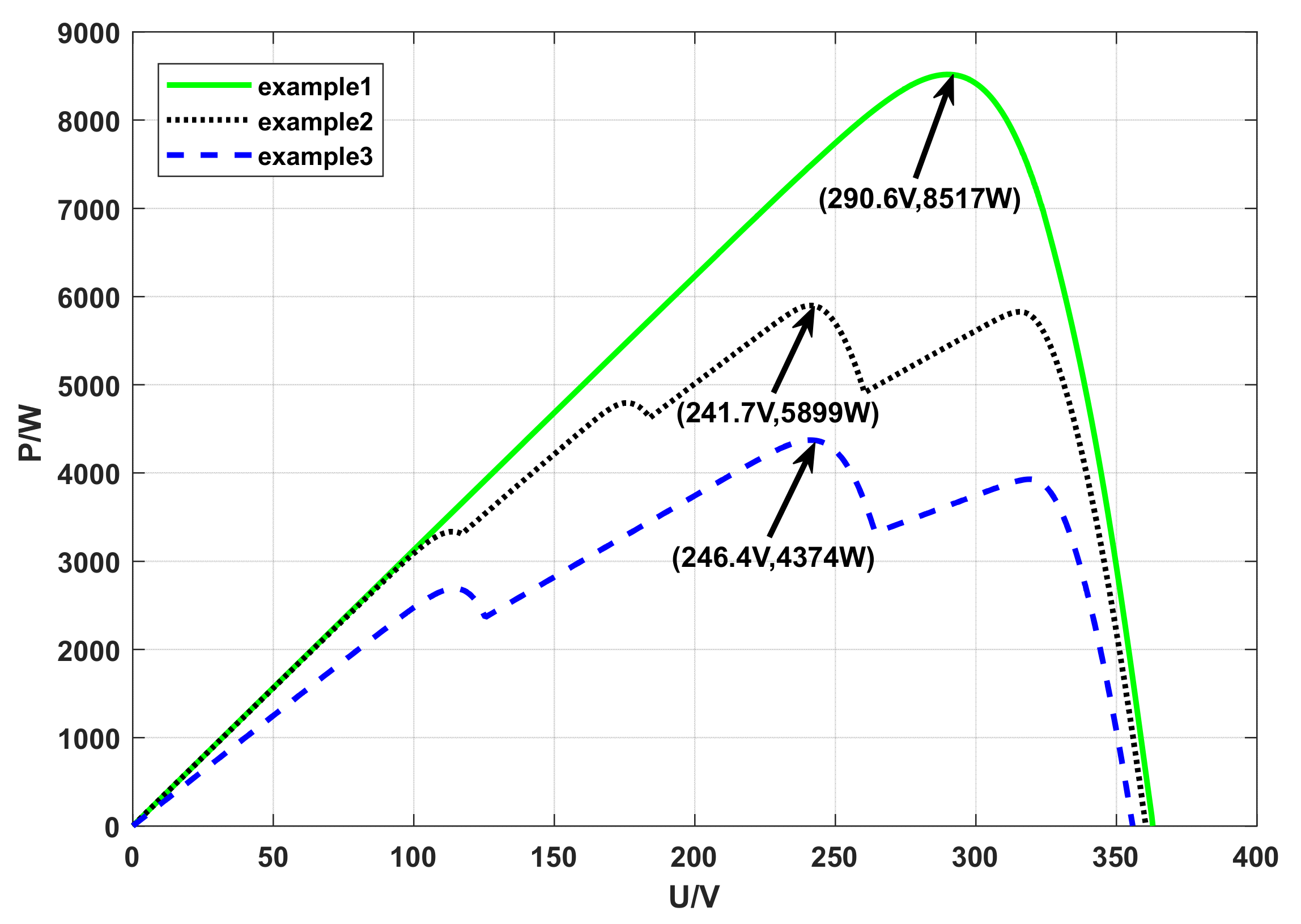
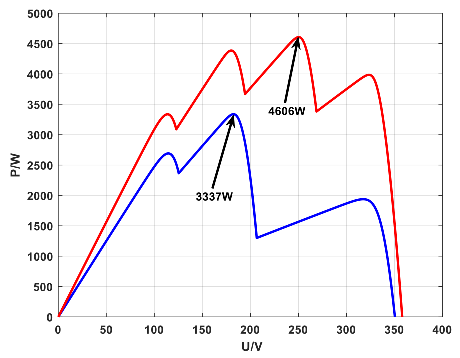
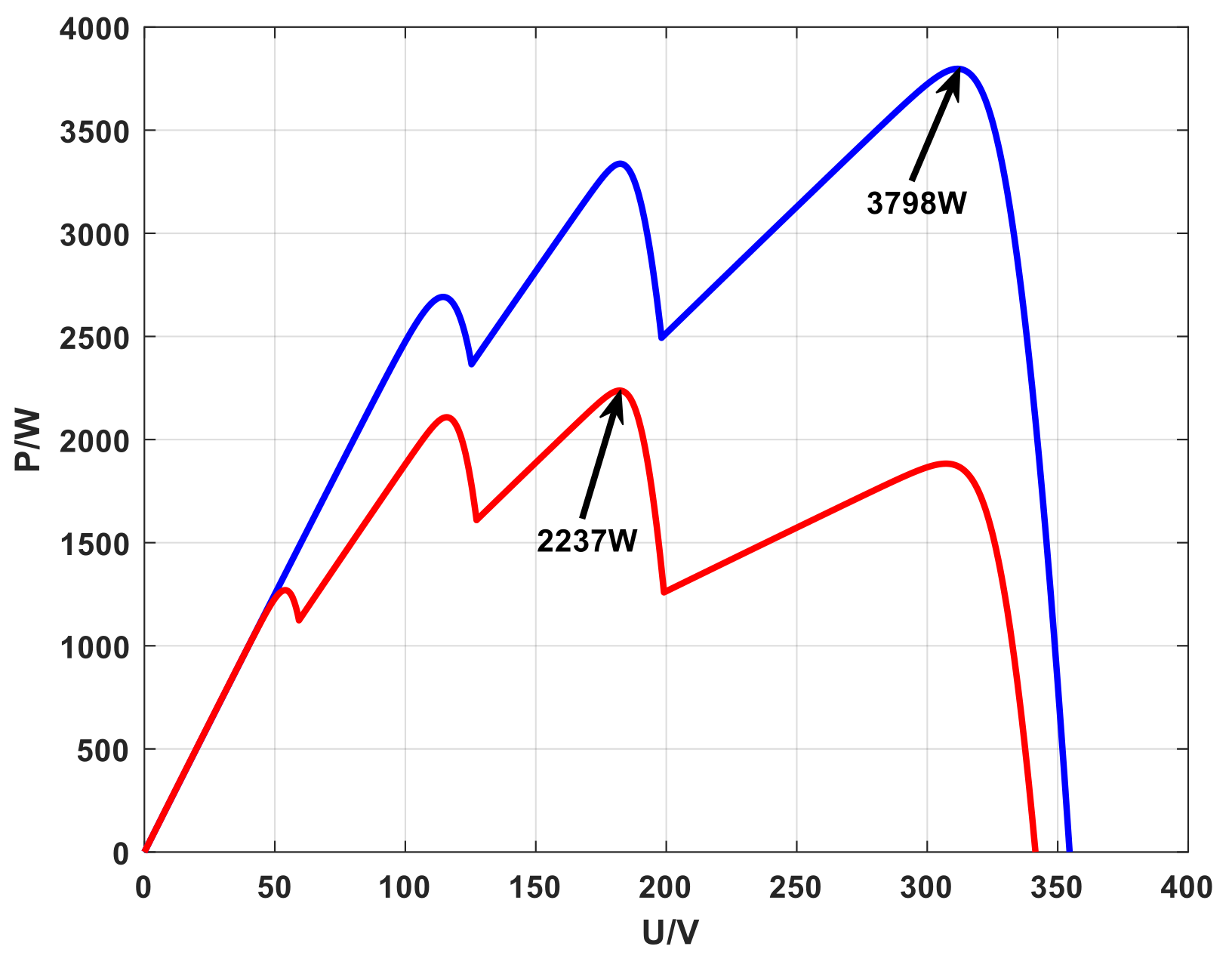
Classic MPPT techniques, including hill climbing (HC) [4,5,6], open circuit voltage (OCV) [7], incremental conductance (INC) [8], perturb and observe (P&O) [9,10,11], and constant voltage (CV) [12,13], are widely used due to their low complexity and cost-effectiveness. These algorithms are effective in uniform irradiation conditions and can accurately track the MPP [14]. However, they may experience oscillations when searching around the MPP, resulting in slow convergence and power loss. Moreover, classic MPPT algorithms have a limited capacity to respond quickly to changes in shading conditions, preventing them from effectively tracking the MPP. As a matter of fact, the output power for solar PV systems can be influenced by environmental and weather factors such as the shadows of trees, buildings around the PV power station, moving clouds, and temperature. This situation is defined as partial shading conditions (PSCs), where each PV panel may simultaneously encounter differing solar irradiance and temperatures. Under different PSCs, PV systems exhibit nonlinear power–voltage (P-V) characteristics with multiple peaks of power [15]. These peaks correspond to local maximum power points (LMPPs), with a sole global maximum power point (GMPP) also present. The conventional MPPT algorithm has many problems in PSCs. The problems include failing to jump out of the LMPP, low optimization efficiency, and inaccuracy. In recent years, many scholars have effectively solved the problem of tracking GMPP through the utilization of metaheuristic optimization methodologies, with examples such as the ant colony optimization algorithm (ACO) [16], grey wolf algorithm (WOA) [17,18], firefly algorithm (FA) [19,20], artificial bee colony algorithm (ABC) [21,22], etc.

The particle swarm optimization (PSO) algorithm [23] is extensively used in the field of MPPT. The PSO algorithm has the advantages of low memory requirement and comparatively fast convergence speed. In the reference [24], a novel approach was proposed where each PV module was treated as a particle, and the MPP was considered as the moving element. Compared with the P&O method, this method improved the efficiency by over 12% in the transient state. The modified PSO (MPSO) method was proposed for a multilevel inverter-based PV system in the reference [25]. This MPSO method introduced cognitive components and worst-experience social components to enhance the speed of searching for the MPP. A combination of the modified PSO and P&O methods in the reference [26] was applied. This method used the adaptive sensitivity parameter to detect the GMPP and tracked GMPP faster and more accurately. An MPV-PSO algorithm based on modified particle velocity of PV systems under PSCs was discussed in the reference [27], which achieves a balance between adaptive and deterministic features. Moreover, it could solve problems like particles getting trapped in LMPPs. A logarithmic particle swarm optimization (LPSO) method in PV systems was proposed in the reference [28], which updates particle velocity solely based on the direction of the GMPP. It should be noted that the PSO algorithm requires multiple iterations to converge. Furthermore, the main drawback of the PSO algorithm is that it frequently tends to adhere to the first local peak rather than effectively tracking the dynamic movement of the global peak, particularly when shading conditions vary over time.

In 2018, the Butterfly Optimization Algorithm (BOA) [29] was presented by the authors Arora and Singh. The BOA has been widely recognized for its strong search capabilities and effectiveness in converging toward the global maximum point with a high degree of accuracy. It has been extensively discussed by many scholars. For instance, the work in [30] is presented to validate the proposed chaotic algorithm on single mode, multimodal, and engineering design problems. The work in [31] has been proposed to optimize the analysis of annual cost, energy consumption, energy efficiency, and pollutant reduction. Despite numerous applications of the BOA in various areas, such as microgrid optimization scheduling, parameter adjustment, and other domains, its application in MPPT is still relatively limited. In the reference [32], the BOA method was applied to PV systems with the aim of mitigating the negative impact of shading and improving the tracking speed. A modified version of the BOA was proposed in the reference [33], which used a single dynamic variable as the tuning parameter, resulting in reduced algorithm complexity. In the reference [34], a method was presented to solve power point fluctuations between GMPP and LMPPS, leveraging an opposition-based reinforcement learning methodology in conjunction with the BOA. Based on the above research, it can be found that there exist some deficiencies in the BOA, such as long convergence time, as well as large oscillations during optimization.

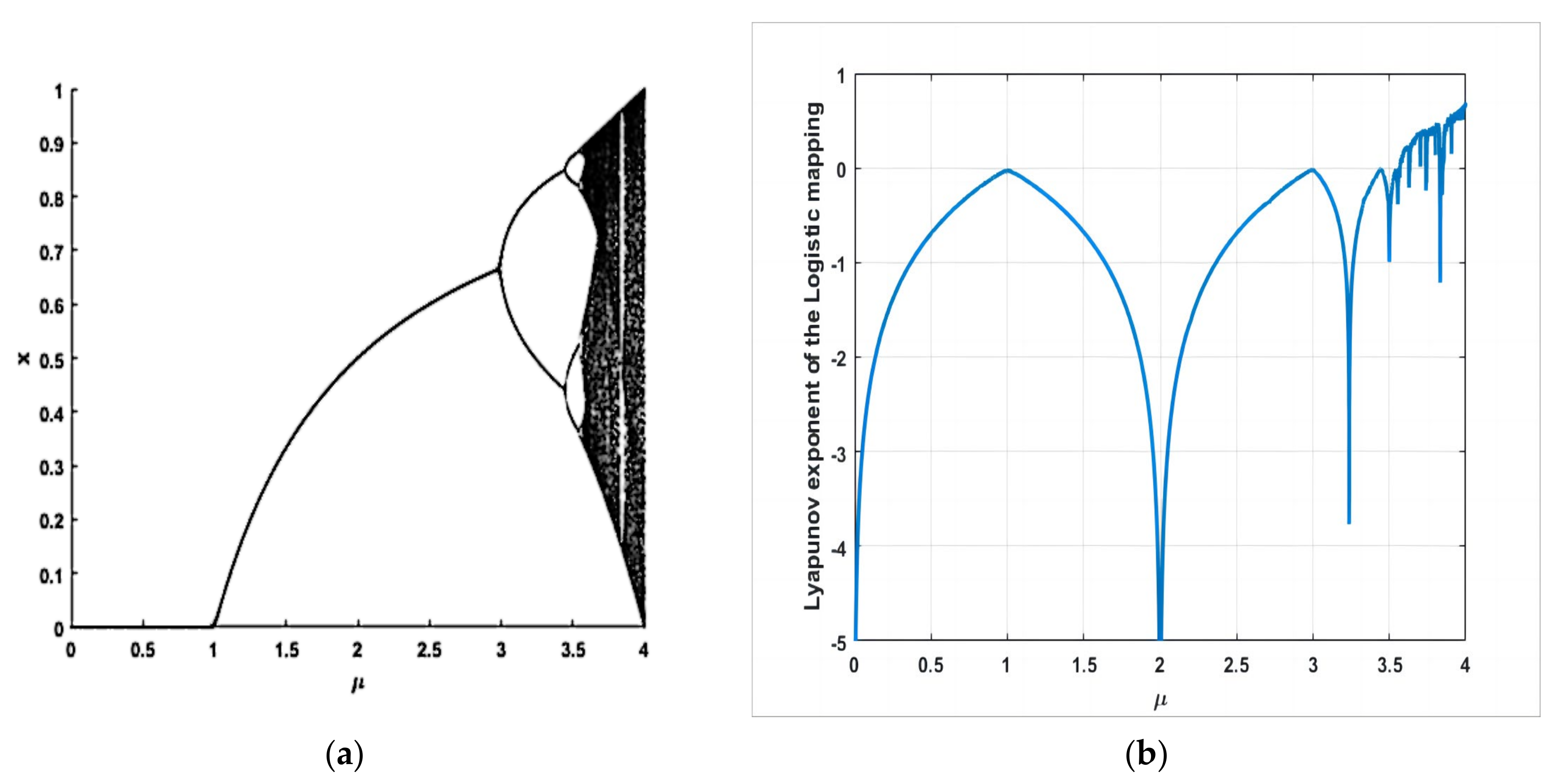
Motivated by the research mentioned above, this paper introduces an innovative PSO-BOA algorithm for solving the slow convergence issues in the BOA while incorporating the advantages and strong robustness of the PSO algorithm. Compared to the traditional PSO and BOA methods, the proposed PSO-BOA algorithm effectively combines the benefits of both approaches while overcoming their respective shortcomings, such as the low convergence accuracy of PSO and the slow convergence and large oscillation of the BOA. Under PSCs, the PSO-BOA algorithm demonstrates remarkable accuracy in tracking the GMPP, exhibiting superior tracking speed, efficiency, and reduced oscillation. With the goal of enhancing the optimization performance of the PSO-BOA algorithm, this article introduces two modifications: a control parameter of sensory modality based on logistic mapping and the self-adaptive adjustment of the inertial weight. The simulation results suggest that the proposed algorithm effectively addresses the shortcomings of existing MPPT algorithms and offers a promising alternative for practical application in various renewable energy systems.

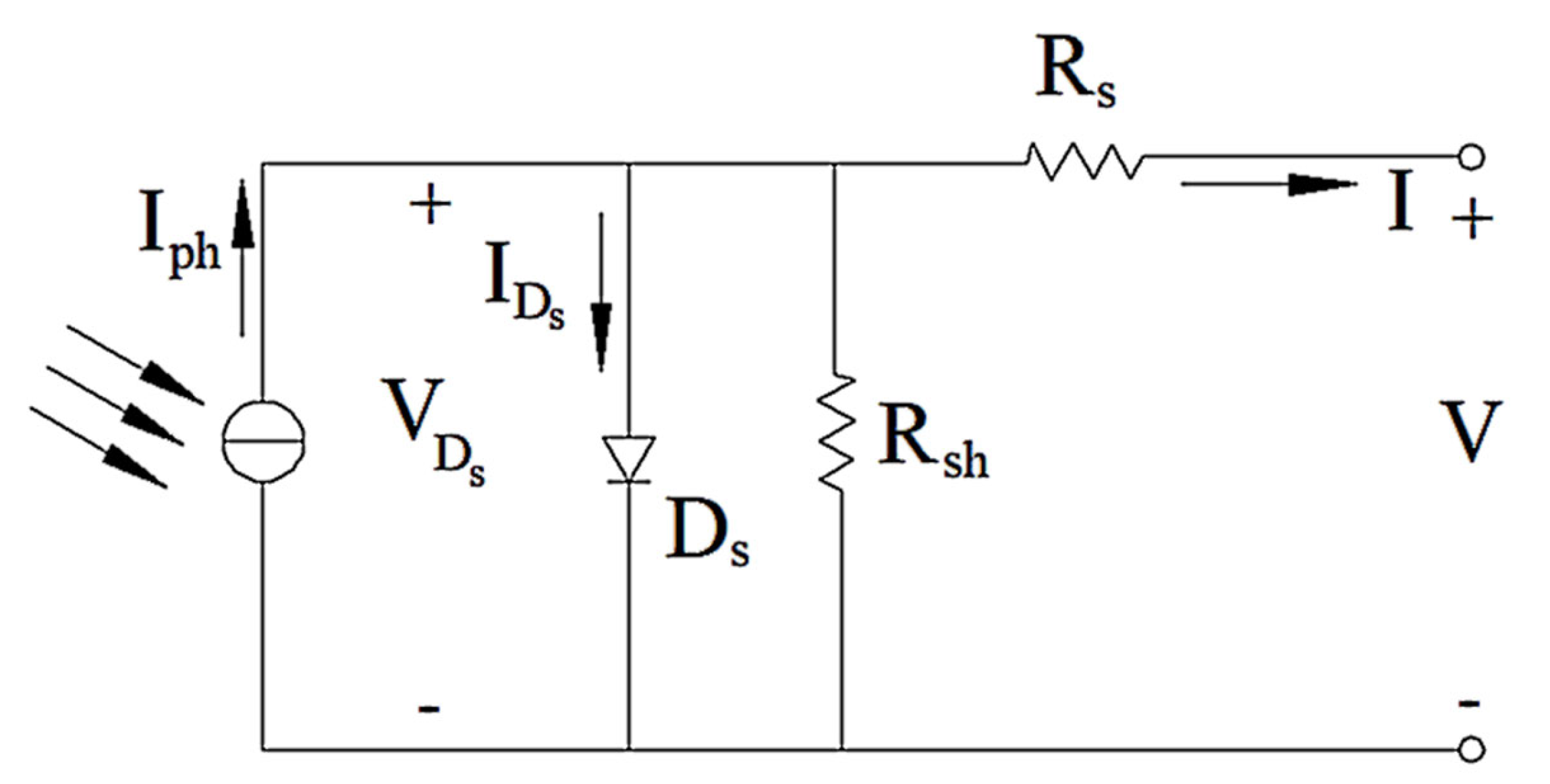
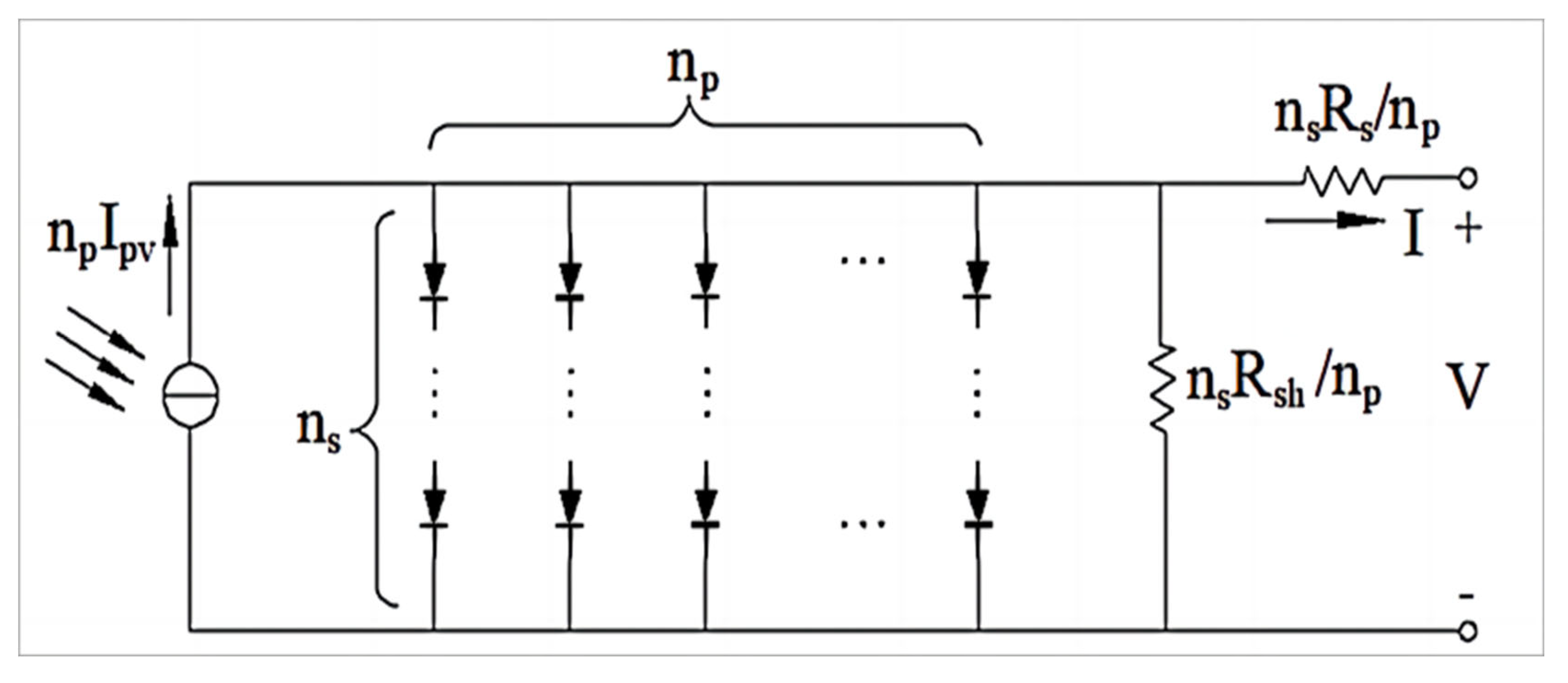
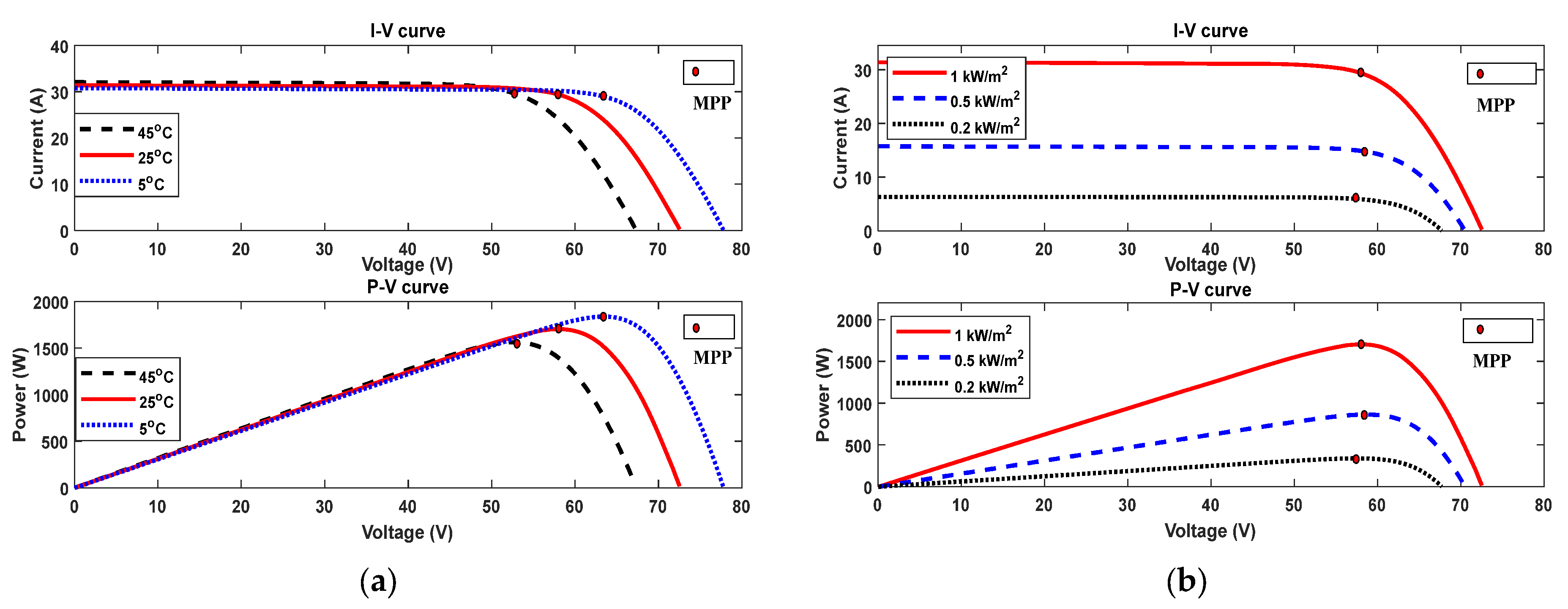
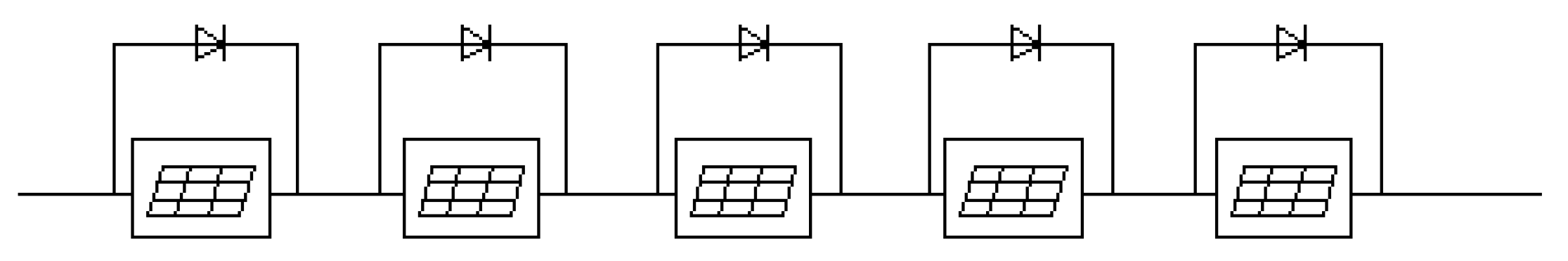
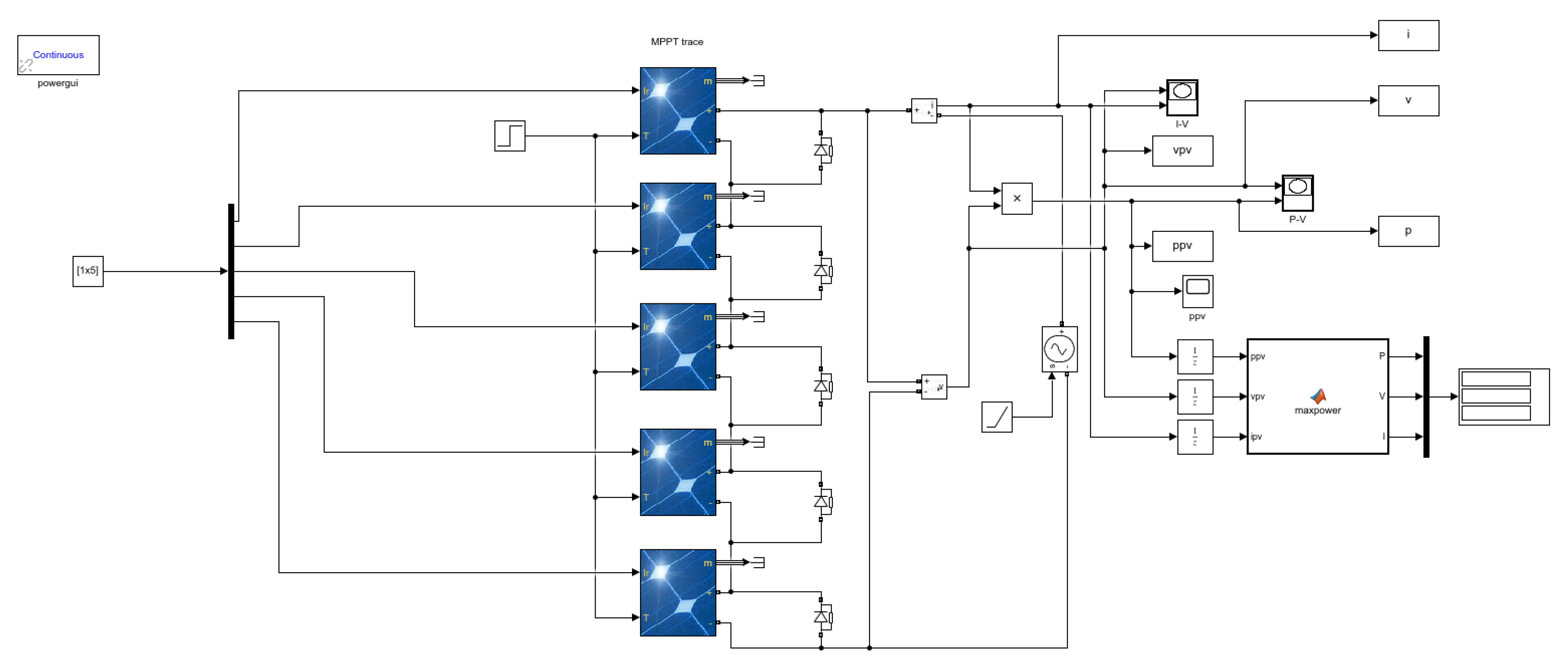
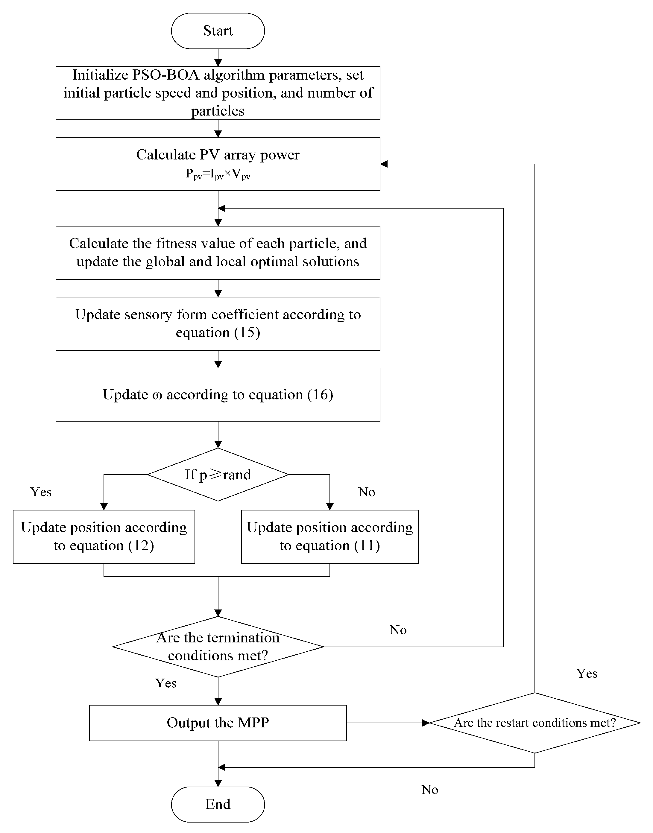
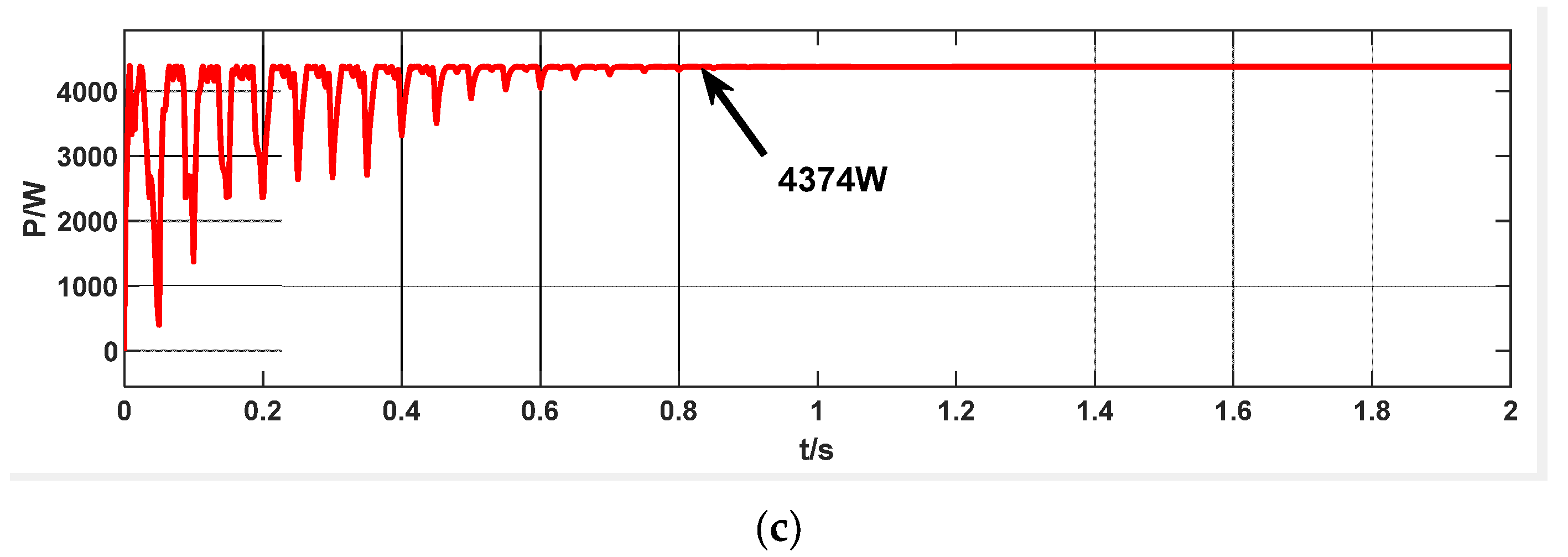
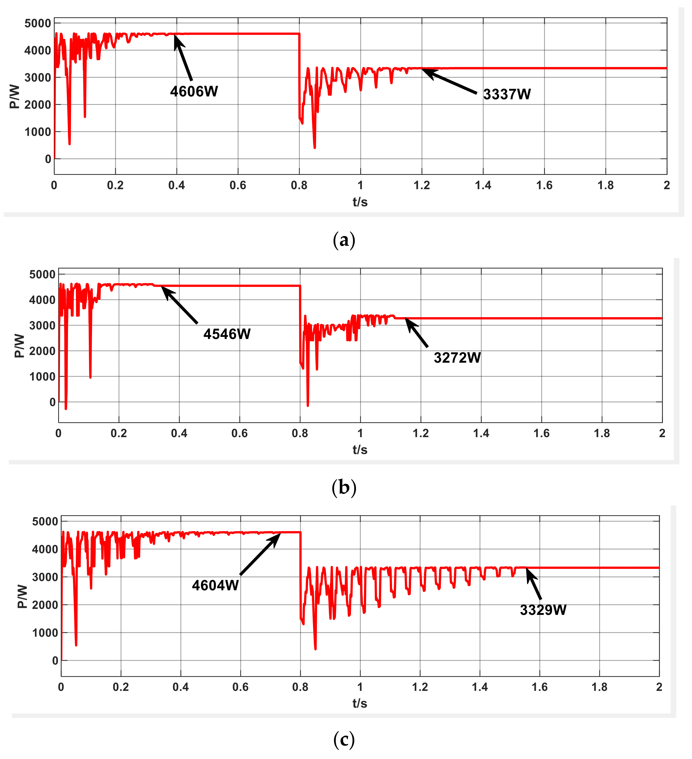
The subsequent sections of this article are structured as follows: Section 2 provides an overview of the multi-peak output characteristics under PSCs. Section 3 introduces the PSO-BOA algorithm utilized to control the PV system. Section 4 presents an analysis of the simulation results from MPPT techniques based on PSO-BOA, BOA, and PSO, respectively. Finally, Section 5 provides a summary of the key findings discussed in this paper.

2. Characteristics of Photovoltaic Array under Partial Shading Conditions

2.1. Mathematical Model of Photovoltaic Cells

A PV cell is a semi-conductor material that absorbs energy from sunlight and allows its electrons to jump to higher energy states. The liberated electrons subsequently undergo free movement along connected conductive wires, resulting in the generation of an electric current. This phenomenon of PV conversion is called the PV effect [35]. It harnesses the PV effect to directly transform solar energy into electrical energy. Figure 1 represents the single-diode model of a solar cell.

Applying Kirchhoff’s current law [36], the output current is represented as follows:

$$I=I_{ph}-I_{D_{\mathrm{s}}}-I_{sh}=I_{ph}-I_{D_{\mathrm{s}}}-\frac{V+I{R}_s}{R_{sh}}$$

(1)

where I represents the current through series resistor $R_s$, $I_{sh}$ is the current through shunt resistor $R_{\mathrm{sh}}$, $I_{ph}$ is the photo-generated current, $V_{D_{\mathrm{s}}}$ is the voltage across $D_s$, and $I_{D_{\mathrm{s}}}$ is the current through the diode $D_s$. The output voltage of the solar cell is represented by V.

The following Shockley equation [37] can be used to express the electric current:

$$I_{D_{\mathrm{s}}}=I_0\left({{\displaystyle e}}^{\frac{qV{D}_{\mathrm{s}}}{\eta KT}}-1\right)=I_0\left({{\displaystyle e}}^{\frac{q\left(V+R_{S}I\right)}{\eta KT}}-1\right)$$

(2)

where $\eta$ is the ideality factor of the diode; $K$ is the Boltzmann constant, K = 1.38 × 10⁻²³ J/K; T is the ambient temperature; q is the electronic charge constant, q = 1.6 × 10⁻¹⁹ C; $R_s$ is the equivalent series resistance; V is the output voltage of the PV array; and I is the output current of the PV array.

By substituting Equation (2) into Equation (1), the I-V characteristic model is derived and represented as follows:

$$I=I_{ph}-I_0\left({{\displaystyle e}}^{\frac{q\left(V+R_{S}I\right)}{\eta KT}}-1\right)-\frac{V+I{R}_S}{R_{\mathrm{sh}}}$$

(3)

A PV module commonly consists of numerous solar cells arranged in a series or in parallel to effectuate increased power, voltage, and current output levels. This unique design also allows PV modules to adapt to various system requirements and environmental conditions. The series configuration enables the module to generate higher voltages, making it suitable for applications that demand higher voltage levels. In contrast, the parallel arrangement ensures that sufficient current is provided, which is ideal for situations where higher current output is essential. The output characteristic is influenced by both its internal parameters and external factors, such as temperature and light intensity [38]. The equivalent circuit is depicted in Figure 2.

The current-voltage characteristics of a PV module model [39] are represented by Equation (4):

$$I=n_p{I}_{ph}-n_p{I}_{sc}\left(exp\left[\frac{q\left(V+I\frac{n_s}{n_p}\right)}{n_s\eta KT}\right]-1\right)-\frac{\frac{n_{p}V}{n_s}+I{R}_s}{R_{sh}}$$

(4)

where n_p is the number of lateral PV panels, n_s is the number of vertical PV panels, $I_{sc}$ is the saturation current of the diode.

The value of $I_{ph}$ is dependent on the intensity of the light source and temperature.

$$I_{ph}=I_{ph\_STC}+K_i\left(T-T_{ref}\right)\frac{G}{G_{STC}}$$

(5)

where $I_{ph\_STC}$ is the short-circuit current under standard temperature and irradiance intensity; $K_i$ is the temperature coefficient of current change, $K_i$ = 0.003; $T_{ref}$ is the standard temperature, $T_{ref}$ = 25 °C; and G is the current irradiance intensity, while $G_{STC}$ is the standard irradiance intensity, $G_{STC}$ = 1000 W/m².

As stated in Equation (4), the I-V characteristic of PV modules undergoes significant alterations by external factors, such as solar irradiance and ambient temperature. The I-V and P-V curves presented in Figure 3a illustrate how different temperatures, while maintaining the same irradiance level, can influence the performance of the system. With increasing temperature, the I-V curve shifts toward a lower voltage, whereas a decrease in temperature causes the I-V curve to shift toward a higher voltage. Additionally, as indicated by the P-V curve, the power exhibits a negative correlation with the increase in temperature. Figure 3b shows the I-V curve and P-V curve at constant temperatures with varying irradiance. It is evident that a rise in solar irradiance leads to a corresponding increase in current and power. Observing Figure 3a,b, it is apparent that the MPP varies with changes in irradiance and module temperature. Hence, it is imperative to consider the impact of temperature and irradiance on PV solar systems.

2.2. Output Characteristics of Photovoltaic Array under Partial Shading Conditions

Under PSCs, when the incident irradiance on the PV panels decreases, the shaded areas experience heating, leading to the hot spot effect, which can potentially cause damage to the entire panel. To address these issues, bypass diodes are usually connected in parallel with PV cells to prevent temperature rise caused by the hot spot effect. Furthermore, the multi-peak characteristics arising from partial shading are associated with the PV cells connected in series within the array. This paper presents a simulation analysis of the output characteristics of a PV array considering five PV cells under PSCs. The PV array structure is illustrated in Figure 4.

Each PV module configures the parameters in the simulation model described in

Table 1. Simulation model parameters for each PV module.

Parameter	Value
Short-Circuit Current: Isc	7.84 A
Open circuit voltage: Uoc	36.3 V
The voltage of MPP: Um	29 V
The current of MPP: Im	7.35 A

. The simulation tests are carried out under standard irradiance conditions of 1000 W/m² and a standard ambient temperature of 25 °C. These tests are conducted under three different conditions, as detailed in

Table 2. PV panels subjected to different irradiances.

Example	S1 (W/m2)	S2 (W/m2)	S3 (W/m2)	S4 (W/m2)	S5 (W/m2)
1	1000	1000	1000	1000	1000
2	1000	1000	900	800	600
3	800	800	600	600	400

: example 1 remains unshaded, while examples 2 and 3 are subjected to PSCs. Figure 5 illustrates a simulated diagram of the photovoltaic components tracking the MPP theory, while Figure 6 presents the P-V characteristic curve. The pseudo-code for obtaining the theoretical MPP is outlined in Algorithm 1, where the theoretical MPP and the corresponding P-V curve are derived using the same method as described in this paper.

Algorithm 1. Pseudo-code of getting theory MPP

1. Setting the irradiance and temperature received by five solar panels.

2. Initialize the parameter of Pmax = 0, Imax = 0, Vmax = 0.

3. Input power current voltage of five solar panels

4. If Pmax < power

5.    Pmax = power

6.    Imax = current

7.    Vmax = voltage

8. End if

9. Return Pmax, Imax, Vmax.

It can be observed that under non-standard irradiance intensity, the PV array demonstrates the occurrence of multiple peaks in its power output characteristic curve. The number of peaks and the power vary with the degree of shadowing. Therefore, accurately tracking the GMPP is crucial under PSCs.

3. The Proposed Algorithm of Particle Swarm Optimization–Butterfly Optimization Algorithm

3.1. The Particle Swarm Optimization (PSO)

PSO [23] is a swarm intelligence optimization algorithm that mimics the search for food by a moving flock of birds in a multidimensional search space. PSO is widely adopted in solving optimization problems of nonlinear systems, owing to its advantages of rapid convergence and straightforward implementation. The velocity and position update formulas in the PSO algorithm are, respectively, expressed in Equations (6) and (7):

$$v_i^{t+1}=\omega ·v_i^t+c_1·ran{d}_1\left(p_{best}-x_i^t\right)+c_2·ran{d}_2\left(g_{best}-x_i^t\right)$$

(6)

$$x_i^{t+1}=x_i^t+v_i^{t+1}$$

(7)

where $v_i^t$ and $v_i^{t+1}$ are the velocities of the i-th particle at the (t) and (t + 1) iterations; $p_{best}$ and $g_{best}$ represent the local and global optimal positions of particles. Generally, $c_1$ and $c_2$ are the acceleration factors. In the reference [23], the stochastic factors (rand₁ and rand₂) were multiplied by a factor of 2 to achieve a mean value of 1. This adjustment was made to ensure that the particles would “overfly” the target about half of the time. Therefore, the $c_1$ and $c_2$ are equal to 2 in this paper; rand₁ and rand₂ are the random numbers that range from 0 to 1; $\omega$ represents the inertia weight.

3.2. The Butterfly Optimization Algorithm (BOA)

The BOA [29] mimics the habits of butterflies searching for food and seeking mates in their natural habitat. Setting the BOA apart from other optimization algorithms is that each butterfly in the algorithm is equipped with its own unique odor, leading to the generation of distinct odor intensities between individuals. By releasing a higher level of odor intensity, a butterfly can attract and be perceived by neighboring butterflies. The intensity of an individual’s odor is perceived by other butterflies, which is denoted by Equation (8):

$$f\left(x\right)=c{I}^a$$

(8)

where $f\left(x\right)$ represents the perceived magnitude of fragrance; c is the sensory modality; I corresponds to the stimulus intensity; and a is the power exponent that relates to the degree of fragrance absorption and is limited to [0, 1].

In theory, the sensory modality coefficient c can be assigned a value within the range [0, ∞]. However, in the iterative process, the specific value of c is determined by the particular optimization problem. During the optimal search phase of the algorithm, the sensory modality c is expressed using the following formulation:

$$c_{t+1}=c_t+\left[\frac{0.025}{c_t·T_{\max }}\right]$$

(9)

where $T_{\max }$ represents the upper bound of the number of iterations; generally, the initial value of parameter $c_t$ is 0.01 [40].

Butterflies are capable of finding food and mating partners through both global and local search strategies in nature. The BOA utilizes a switching probability, denoted as “p”, that governs the shift from a wide-ranging global exploration to a concentrated local exploration. Based on a comparison of the switching probability ‘p’ with a random number, the BOA decides whether to execute a local search or a global search. The position updating formula is demonstrated by Equation (10), as follows:

$$x_i^{t+1}=\left\{\begin{array}{l}{x}_i^t+(r^2·g^{\ast }-x_i^t)f_i p<rand\\ x_i^t+(r^2·x_a^t-x_b^t)f p\ge rand\end{array}\right.$$

(10)

where $g^{\ast }$ is the current best-performing one in all the solutions that have been generated in the current stage; $x_a^t$ and $x_b^t$ represent the spatial positions of the a-th and b-th butterflies in the t-th iteration, and when a = b, the butterfly performs a local random search; r is a number that is generated randomly, 0 < r < 1; and $f_i$ is the fragrance produced by the i-th butterfly.

3.3. The Particle Swarm Optimization–Butterfly Optimization Algorithm

In the process of searching, it is simple for the PSO algorithm to fall into the local optimal solution. The main drawback of the BOA is its extended convergence time and significant oscillations during the process. To address the limitations of the PSO and BOA algorithms, the PSO-BOA algorithm incorporates the BOA search mechanism into the PSO algorithm. Specifically, the algorithm selects the search method based on comparing the generated random number with the predetermined switching probability ‘p’. To enhance the algorithm’s ability to identify the global optimal value, the PSO-BOA algorithm integrates two strategies. On the one hand, the strategy randomizes the spatial position of individual particles during the local search process, which explores a diverse search space and optimizes the quality of individual particles. On the other hand, the strategy utilizes both local and global optimal particles to update the position and speed of particles in the global search process, enabling the algorithm to exploit the current best solutions and refine the search trajectory toward the global optimal value. Simultaneously, the PSO-BOA algorithm adjusts the sensory modality c and the inertia weight $\omega$ in the iteration process, which accelerates the convergence rate and improves the local search performance.

3.3.1. Global Search

The updating criterion of the position for the global search stage in the PSO-BOA algorithm can be represented by Equation (11) as follows:

$$x_i^{t+1}=x_i^t+\left(\omega ·v_i^t+c_1·ran{d}_1·\left(p_{best}-x_i^t\right)+c_2·ran{d}_2·\left(g_{best}-x_i^t\right)\right)f_{\max }$$

(11)

where $v_i^t$ is the velocity of the i-th particle at the t-th iteration; $p_{best}$ and $g_{best}$ represent the local and global optimal positions of particles; and $f_{\max }$ represents the current optimal scent intensity value. Generally, $c_1=c_2=2$; rand₁ and rand₂ generate a random number that falls between 0 and 1. $\omega$ represents the inertia weight.

3.3.2. Local Search

The updating of the position formula for the local search stage used in the PSO-BOA algorithm can be represented by Equation (12) as follows:

$$x_i^{t+1}=x_i^t+\left(r^2·\left(x_{\mathrm{a}}^t-x_i^t\right)-\omega ·\left(x_{\mathrm{b}}^t-x_i^t\right)\right)f_i$$

(12)

where $x_{\mathrm{a}}^t$ and $x_{\mathrm{b}}^t$ are the spatial positions of the a-th and b-th butterflies in the t-th iteration; the parameter $\omega$ represents inertia weight; r generates a random number that falls between 0 and 1.

3.3.3. Parameter Control Strategy

Chaos theory has numerous applications in intelligent optimization algorithms. Logistic mapping [41] is one of the classic chaotic mapping methods in chaos theory, and its representation is shown in Equation (13):

$$z_{l+1}=\mu z_l\left(1-z_l\right)$$

(13)

where $\mu$ is the chaotic parameter, and the value falls in [0, 4], l can be defined as the iteration count of the chaotic map.

The Lyapunov index [42] is a measure for distinguishing chaotic characteristics. A larger value of the Lyapunov exponent indicates a higher degree of chaos and stronger chaotic characteristics. The Lyapunov exponent is calculated by Equation (14):

$$\lambda =\underset{n\to \infty }{{\displaystyle \lim }}\frac{1}{n_h}{\displaystyle \sum _{i=0}^{n_h-1}\ln \left|f^{\prime }\left(z_i\right)\right|}$$

(14)

where $\lambda$ is the Lyapunov exponent; $n_h$ is the number of iterations of the map function; and $f^{\prime }\left(·\right)$ is the first derivative of the chaotic map function.

Produce a logistic diagram and a Lyapunov exponent curve of the logistic map where parameter $\mu$ is within the interval (0, 4], as illustrated in Figure 7.

As illustrated in Figure 7, the bifurcation of the logistic map occurs at $\mu$= 3.55, and with an increase in the parameter value, the range of the map gradually expands to (0, 1). When $\mu$ = 4, the logistic map exhibits chaotic behavior, leading to a sequence within the range (0, 1). The maximum Lyapunov exponent of the logistic map is calculated to be 0.6839. Consequently, the parameter $\mu$ is set to 4.

According to the logistic mapping expression, the sensory modality c in the PSO-BOA algorithm can be represented by Equation (12) as follows:

$$c\left(t\right)=4·c_0\left(t-1\right)\left(1-c_0\left(t-1\right)\right)$$

(15)

The coefficient of inertia weight directly affects the particle flight speed of the PSO algorithm. A dynamic tuning strategy is utilized to alter the local and global search capabilities of the algorithm, as depicted in Equation (16):

$$\omega ={\omega }_1-\left({\omega }_1-{\omega }_2\right){\left(\frac{t}{T_m}\right)}^2$$

(16)

where ${\omega }_1$ represents the initial inertia weight; ${\omega }_2$ represents the inertia weight at the maximum number of iterations; t represents the current number of iterations; and $T_m$ represents the maximum number of iterations. In this paper, the initial value of the inertia weight is set to 0.9, and the inertia weight value of the last iteration is set to 0.2. As the iteration progresses, the inertia weight decreases from 0.9 to 0.2. A larger inertia weight in the initial stage of the iteration can maintain the strong global search ability of the algorithm, while a smaller inertia weight in the later stage of the iteration is conducive to accurate local search and facilitates algorithm convergence.

3.4. Particle Swarm Optimization–Butterfly Optimization Algorithm for Maximum Power Point Tracking of Photovoltaic Arrays System

The input variables are the current I and voltage V of PV arrays, and the duty cycle D is the particle of individuality. Simultaneously, the duty cycle D is the output variable, which is controlled by regulating the MOSFET switching behavior to achieve the desired on and off states. The flowchart of the PSO-BOA algorithm proposed in this paper is presented in Figure 8. The pseudo-code of the PSO-BOA algorithm in this paper is presented in Algorithm 2 [43].

Algorithm 2. Pseudo-code of PSO-BOA algorithm

1.Generate the starting population of the particles Xi (i = 1, 2, ..., n) randomly

2.Initialize the acceleration factors c1, c2, power exponent a and switch probability p

3.Calculate the value (fi) of each particles

4.Calculate PV array power Ppv = Ipv×Upv

5.While t = 1: the upper limit of iterations

6.     For each search of the particles

7.           Update the fragrance f according to Equation (8)

8.      End for

9.      Find the best f (fmax)

10.     For each search of the particles

11.         Set a random number “rand” in [0, 1]

12.           If rand < p then

13.               Move to the best position according to Equation (12)

14.           Else

15.               Move to adjust positions according to Equation (11)

16.           End if

17.     End for

18.               Update the velocity v according to Equation (6)

19.               Calculate the new fitness f value of each particles

20.           If fnew < fmax

21.             Update the position of best f according to Equation (7)

22.           End if

23.        Update the value of sensory modality c according to Equation (15)

24.        Update the value of inertia weight $\omega$ according to Equation (16)

25. t = t + 1

26.End while

27.If reach the restart condition as Equation (17)

28.Return to line 5

29. End if

30.Output the MPP

When the termination condition is reached, the value of maximum power for the PV array is output; otherwise, the search continues. Additionally, during dynamic local shading, the output of the P-V characteristics also changes. To determine whether the algorithm needs to be restarted by detecting the degree of power change, this article defines the restart condition as shown in Equation (17).

$$\Delta P=\frac{P_m^k-P_m}{P_m}$$

(17)

where $P_m^k$ is the effective output power value after local shading changes; $P_m$ is the maximum power output value before local shading changes.

4. Simulation Results

A comparative analysis is performed for the PSO-BOA, PSO, and BOA algorithms proposed in this study in order to assess their effectiveness for MPPT under four different irradiance conditions, namely, standard irradiance conditions, local shading conditions, abrupt alterations for irradiance conditions, and sudden variations for irradiance and temperature conditions. When analyzing scenarios with uniform irradiance, we compared the PSO-BOA algorithm with the P&O, PSO, and BOA algorithms. In this case, the P&O algorithm is configured with a perturbation step size of 0.005. The population size is set to 10, and maximum iteration count is set to 15 for all three algorithms. The basic parameters of these algorithms are presented in

Table 3. Parameters of three algorithms.

Algorithm	Related Parameters
PSO-BOA	a = 0.4, c0 = 0.35, ${\omega }_1$ = 0.9, ${\omega }_2$ = 0.2, $c_1=2$, $c_2=2$, $p=0.8$
PSO	$\omega$ = 0.4, $c_1=2$, $c_2=2$
BOA	a = 0.4, c0 = 1, $p=0.8$

. This study utilizes a boost circuit for the PV array, which was controlled by MPPT, as depicted in Figure 9. In this study, the system uses a PV array comprising five PV panels in series. The parameters of the boost circuit are designed as follows: Cpv = 500 μF, L = 0.85 mH, C = 200 μF, R = 30 Ω, and the MOSFET frequency is set at 0.1 MHz.

4.1. Optimization Results under Uniform Irradiance

Under a standard light intensity of 1000 W/m² and a standard ambient temperature of 25 °C, it is observed that the output power demonstrated a single peak characteristic. The P-V characteristic of the output is depicted in Figure 10. Specifically, the GMPP of the PV arrays is observed to be 8517 W.

The GMPP is searched using the aforementioned four algorithms in this article. Figure 11 presents the simulation results for these four algorithms, with a simulation time of 2 s.

Figure 11 demonstrates that all four algorithms (PSO-BOA, PSO, P&O, and BOA) are capable of tracking GMPP under uniform irradiance. In this situation, the P&O algorithm can track the MPP relatively quickly, but it suffers from significant oscillations and fails to converge to the MPP. Therefore, this paper does not provide further comparisons for the other complex conditions. When reaching the stable state, the power tracked by the other three algorithms is 8517 W, which is the theoretical maximum power. However, the convergence rate of the three algorithms varies. The PSO algorithm converges rapidly but tends to exhibit fluctuations around the maximum power point for an extended period of time, whereas the BOA has the slowest convergence rate. The PSO-BOA algorithm requires the least amount of time and significantly improves the convergence speed.

4.2. Optimization Results during Static Shading

In the setting of standard ambient temperature conditions at 25 °C, each of the five PV panels is subjected to varying light intensities: 800 W/m², 800 W/m², 600 W/m², 600 W/m², and 400 W/m². In this situation, the output power of the PV array exhibits multi-peak characteristics, with the GMPP measuring at 4374 W, as depicted in Figure 12.

The GMPP at this time is determined using the three algorithms mentioned earlier. The simulation curves of these algorithms with a simulation time of 2 s are depicted in Figure 13.

Figure 13 shows that both the PSO-BOA and BOA algorithms have the capability to track the theoretical GMPP accurately. However, the PSO algorithm tracks a slightly lower GMPP of 4373 W, with a deviation value of 1 W, and exhibits small oscillations even reaching the steady state (after 0.4 s). In contrast, the BOA has slower convergence and larger power oscillations. Under static shading conditions, the PSO-BOA algorithm displays significant improvement in convergence speed and reduction in power oscillation.

4.3. Optimization Results under Abrupt Alterations for Irradiance Conditions

To test the response of a PV array to rapid changes in light intensity, this paper conducts a series of tests involving exposing the array to different light intensities at specific time intervals. Specifically, the array is devised to varying light intensities of 1000 W/m², 1000 W/m², 800 W/m², 800 W/m², and 400 W/m² from 0 to 0.8 s, and is then designed by 800 W/m², 800 W/m², 600 W/m², 400 W/m², and 400 W/m² from 0.8 to 2 s. These simulations are carried out under the environmental temperature of 25 °C, and the resulting P-V characteristics are depicted in Figure 14. During the two stages, the corresponding GMPP values of the array are 4606 W and 3337 W. Further evaluation of the system’s performance is conducted by comparing the dynamic shading simulations for three algorithms with a simulation time of 2 s. The comparison is depicted in Figure 15.

Figure 15 shows that the PSO-BOA algorithm accurately tracks the theoretical GMPP under varying irradiance conditions. The BOA also displays good performance in this regard, albeit with a slight tracking error. However, the PSO algorithm exhibits a significant deviation from the theoretical GMPP and is susceptible to local optima, thus resulting in low convergence accuracy. Furthermore, in terms of convergence time, the BOA requires around 0.7 s to converge, with more oscillations during varying irradiance conditions. In contrast, the PSO algorithm has relatively faster convergence, requiring about 0.4 s. Meanwhile, the PSO-BOA algorithm exhibits the fastest convergence time of about 0.3 s, accompanied by less oscillation, thereby demonstrating its superior tracking performance under dynamic local shading conditions. Overall, compared to both the PSO and BOA algorithms, the PSO-BOA algorithm offers improved tracking accuracy and less oscillation.

4.4. Optimization Results under Sudden Variations for Irradiance and Temperature Conditions

To evaluate the output power characteristics under harsh environmental conditions considering the influence of temperature on MPP, this paper sets the irradiance intensity of the array as 800 W/m², 800 W/m², 600 W/m², 400 W/m², and 400 W/m² at 0–0.8 s, while the ambient temperature is maintained at 25 °C. Later, from 0.8 to 2 s, the array experience suddenly changes light intensity to 800 W/m², 600 W/m², 400 W/m², 200 W/m², and 200 W/m², while the environmental temperature is increased to 30 °C. The resulting P-V characteristics outputs are depicted in Figure 16, where the GMPP for the two stages is 3798 W and 2237 W. Figure 17 shows the dynamic shading simulations for three algorithms under harsh environmental conditions.

According to the findings illustrated in Figure 17, the PSO-BOA algorithm successfully tracks the theoretical GMPP with high precision. In contrast, the PSO algorithm is prone to falling into local optima after abrupt changes in irradiance and temperature, leading to significant deviations from the theoretical GMPP. Although the BOA can track the theoretical GMPP, the error is still greater than that of the PSO-BOA algorithm. As for convergence speed, the PSO-BOA algorithm shows the fastest convergence speed and the least oscillation. Conversely, the PSO algorithm converges extremely slowly after a sudden change in conditions, oscillating around GMPP. The BOA converges slowly with a large power oscillation amplitude. Notably, in harsh environmental conditions, the PSO-BOA algorithm outperforms different algorithms in the context of both convergence speed and power oscillations.

4.5. Statistics of Results and Analysis

To provide a clearer insight into the performance indicators of each algorithm, statistical tables are created summarizing the results obtained using the above-mentioned three algorithms. The performance of each algorithm is assessed originating from various evaluation metrics, including convergence time, optimization value, projected annual loss cost, and tracking efficiency, as shown in

Table 4. Performance comparison of algorithms.

Example	Statistics	Units	PSO-BOA	PSO	BOA
Uniform irradiance	Convergence time	s	0.43	0.79	0.75
	Optimization value	W	8517	8517	8517
	Theoretical	W	8517	8517	8517
	Projected annual loss cost	¥	0	0	0
	Tracking efficiency	%	100	100	100
	Oscillation situation	/	small	big	big
Static shading	Convergence time	s	0.42	1.12	0.82
	Optimization value	W	4374	4373	4374
	Theoretical	W	4374	4374	4374
	Projected annual loss cost	¥	0	2.19	0
	Tracking efficiency	%	100	99.98	100
	Oscillation situation	/	small	Less small	big
Abrupt alterations for irradiance conditions	Convergence time	s	0.37/0.35	0.32/0.35	0.74/0.71
	Optimization value	W	4606/3337	4546/3272	4604/3329
	Theoretical	W	4606/3337	4606/3337	4606/3337
	Projected annual loss cost	¥	0/0	131.40/142.35	4.38/17.52
	Tracking efficiency	%	100/100	98.70/98.05	99.96/99.76
	Oscillation situation	/	Less small	small	bigger
Sudden variations in irradiance and temperature conditions	Convergence time	s	0.47/0.37	0.77/0.92	0.76/0.75
	Optimization value	W	3796/2237	3794/2169	3755/2230
	Theoretical	W	3798/2237	3798/2237	3798/2237
	Projected annual loss cost	¥	4.38/0	8.76/148.92	94.17/15.33
	Tracking efficiency	%	99.94/100	99.89/96.96	98.87/99.69
	Oscillation situation	/	small	bigger	bigger

.

As illustrated in Table 4, the PSO-BOA algorithm outperforms both the BOA and PSO in all four simulations, achieving faster and smoother convergence to GMPP. It is worth noting that the PSO-BOA algorithm shows a faster convergence speed. The convergence time of PSO-BOA is 54.43% relative to PSO and 57.33% relative to the BOA under uniform irradiance, and is reduced to 37.5% relative to PSO and 51.22% relative to the BOA under local shading conditions. Based on the local electricity prices and assuming an average daily sunlight duration of 12 h, this study calculates the annual cost of losses. In scenarios with abrupt lighting condition changes, the PSO algorithm results in the highest annual loss cost, whereas the PSO-BOA algorithm proves effective in mitigating these losses and reducing costs. Meanwhile, the PSO algorithm achieves faster convergence in cases of sudden changes in irradiance and temperature, but is more prone to falling into local optima, resulting in the worst convergence accuracy. The convergence rate of the BOA is sluggish, with many oscillations occurring over the course of convergence. In contrast, the PSO-BOA algorithm is able to maintain stable and higher optimization accuracy than both the BOA and PSO across all four simulations. These results suggest that the PSO-BOA algorithm effectively addresses the issues of large search oscillation in the BOA and low optimization accuracy in PSO while also improving convergence speed.

5. Conclusions

In response to the issues of low tracking accuracy and susceptibility to local optima in classical PSO algorithms, as well as the problems of slow convergence speed and large oscillation in the BOA, this study introduces a novel PSO-BOA algorithm based on the PSO and BOA. The paper simulated four different scenarios, and the simulation results demonstrate that the PSO-BOA algorithm outperforms the PSO and BOA in terms of convergence accuracy, with a tracking accuracy of no less than 99.94%. In contrast, the PSO algorithm is prone to becoming trapped in local optima, resulting in a convergence accuracy of only 96.96% when both irradiation and temperature undergo abrupt changes. The PSO-BOA algorithm also surpasses both the PSO and BOA algorithms in handling oscillations. In terms of convergence time, the PSO-BOA algorithm shows a significant improvement. Particularly, in scenarios of abrupt changes in irradiation and simultaneous changes in temperature and irradiation, the convergence time of PSO-BOA is less than 0.5 s, while the BOA takes approximately double the time compared to the PSO-BOA. Moreover, the convergence time of the PSO algorithm is relatively longer, and it tends to converge quickly but may be trapped in local optima. Therefore, the proposed algorithm exhibits faster convergence speed, higher tracking accuracy, and smaller oscillations compared to both the PSO and BOA algorithms, which can effectively enhance power supply reliability and safety.

References

1. Yu, S.L.; Zhang, L.J.; Lu, H.H.; Fernando, T.; Wong, K.P. A DSE-Based Power System Frequency Restoration Strategy for PV-Integrated Power Systems Considering Solar Irradiance Variations. IEEE Trans. Ind. Inform. 2017, 13, 2511–2518. [Google Scholar] [CrossRef]
2. Khemili, F.Z.; Bouhali, O.; Lefouili, M.; Chaib, L.; El-Fergany, A.A.; Agwa, A.M. Design of Cascaded Multilevel Inverter and Enhanced MPPT Method for Large-Scale Photovoltaic System Integration. Sustainability 2023, 15, 9633. [Google Scholar] [CrossRef]
3. He, Z.; Tian, Y. Design and Analysis of Comprehensive Solar Utilization System Based on Photovoltaic Concentration and Spectral Splitting. Processes 2023, 11, 1944. [Google Scholar]
4. Carreon-Bautista, S.; Eladawy, A.; Nader Mohieldin, A.; Sánchez-Sinencio, E. Boost converter with dynamic input impedance matching for energy harvesting with multi-array thermoelectric generators. IEEE Trans. Ind. Electron. 2014, 61, 5345–5353. [Google Scholar] [CrossRef]
5. Xu, W.; Mu, C.X.; Jin, J.X. Novel Linear Iteration Maximum Power Point Tracking Algorithm for Photovoltaic Power Generation. IEEE Trans. Appl. Supercond. 2014, 24, 1–6. [Google Scholar]
6. Liu, H.D.; Lu, S.D.; Lee, Y.L.; Lin, C.H. A Novel Photovoltaic Module Quick Regulate MPPT Algorithm for Uniform Irradiation and Partial Shading Conditions. Processes 2021, 9, 2213. [Google Scholar]
7. Kumar, N.; Singh, B.; Panigrahi, B.K. PNKLMF-Based Neural Network Control and Learning-Based HC MPPT Technique for Multiobjective Grid Integrated Solar PV Based Distributed Generating System. IEEE Trans. Ind. Inform. 2019, 15, 3732–3742. [Google Scholar]
8. Pathak, P.K.; Padmanaban, S.; Yadav, A.K.; Alvi, P.A.; Khan, B. Modified incremental conductance MPPT algorithm for SPV-based grid-tied and stand-alone systems. IET Gener. Transm. Distrib. 2022, 16, 776–791. [Google Scholar] [CrossRef]
9. Ahmed, J.; Salam, Z. An improved perturb and observe (P&O) maximum power point tracking (MPPT) algorithm for higher efficiency. Appl. Energy 2015, 150, 97–108. [Google Scholar]
10. Goud, J.S.; Kalpana, R.; Singh, B.; Kumar, S. A Global Maximum Power Point Tracking Technique of Partially Shaded Photovoltaic Systems for Constant Voltage Applications. IEEE Trans. Sustain. Energy 2019, 10, 1950–1959. [Google Scholar] [CrossRef]
11. Lasheen, M.; Rahman, A.K.A.; Abdel-Salam, M.; Ookawara, S. Adaptive reference voltage-based MPPT technique for PV applications. IET Renew. Power Gener. 2017, 11, 715–722. [Google Scholar] [CrossRef]
12. Femia, N.; Petrone, G.; Spagnuolo, G.; Vitelli, M. Optimization of perturb and observe maximum power point tracking method. IEEE Trans. Power Electron. 2005, 20, 963–973. [Google Scholar] [CrossRef]
13. Bounechba, H.; Bouzid, A.; Nabti, K.; Benalla, H. Comparison of perturb & observe and fuzzy logic in maximum power point tracker for PV systems. Energy Procedia 2014, 50, 677–684. [Google Scholar]
14. Padmanaban, S.; Priyadarshi, N.; Bhaskar, M.S.; Holm-Nielsen, J.B.; Hossain, E.; Azam, F. A Hybrid Photovoltaic-Fuel Cell for Grid Integration with Jaya-Based Maximum Power Point Tracking: Experimental Performance Evaluation. IEEE Access 2019, 7, 82978–82990. [Google Scholar] [CrossRef]
15. Rezk, H.; Fathy, A. Simulation of global MPPT based on teaching-learning-based optimization technique for partially shaded PV system. Electr. Eng. 2017, 99, 847–859. [Google Scholar] [CrossRef]
16. Chao, K.H.; Rizal, M.N. A Hybrid MPPT Controller Based on the Genetic Algorithm and Ant Colony Optimization for Photovoltaic Systems under Partially Shaded Conditions. Energies 2021, 14, 2902. [Google Scholar] [CrossRef]
17. Mohanty, S.; Subudhi, B.; Ray, P.K. A New MPPT Design Using Grey Wolf Optimization Technique for Photovoltaic System Under Partial Shading Conditions. IEEE Trans. Sustain. Energy 2016, 7, 181–188. [Google Scholar] [CrossRef]
18. Darcy Gnana Jegha, A.; Subathra, M.S.P.; Manoj Kumar, N.; Subramaniam, U.; Padmanaban, S. A High Gain DC-DC Converter with Grey Wolf Optimizer Based MPPT Algorithm for PV Fed BLDC Motor Drive. Appl. Sci. 2020, 10, 2797. [Google Scholar] [CrossRef] [Green Version]
19. Watanabe, R.B.; Ando, O.H., Jr.; Leandro, P.G.M.; Salvadori, F.; Beck, M.F.; Pereira, K.; Brandt, M.H.M.; de Oliveira, F.M. Implementation of the Bio-Inspired Metaheuristic Firefly Algorithm (FA) Applied to Maximum Power Point Tracking of Photovoltaic Systems. Energies 2022, 15, 5338. [Google Scholar] [CrossRef]
20. Teshome, D.F.; Lee, C.H.; Lin, Y.W.; Lian, K.L. A modified firefly algorithm for photovoltaic maximum power point tracking control under partial shading. IEEE Trans. Emerg. Sel. Topics Power Electron. 2017, 5, 661–671. [Google Scholar] [CrossRef]
21. Benyoucef, A.S.; Chouder, A.; Kara, K.; Silvestre, S. Artificial bee colony based algorithm for maximum power point tracking (MPPT) for PV systems operating under partial shaded conditions. Appl. Soft Comput. 2015, 32, 38–48. [Google Scholar] [CrossRef] [Green Version]
22. Gong, L.; Hou, G.; Huang, C. A two-stage MPPT controller for PV system based on the improved artificial bee colony and simultaneous heat transfer search algorithm. ISA Trans. 2023, 132, 428–443. [Google Scholar] [CrossRef] [PubMed]
23. Kennedy, J.; Eberhart, R. Particle Swarm Optimization. In Proceedings of the IEEE International Conference on Neural Networks, Perth, Australia, 27 November–1 December 1995. [Google Scholar]
24. Chen, L.R.; Tsai, C.H.; Lin, Y.L.; Lai, Y.S. A biological swarm chasing algorithm for tracking the PV maximum power point. IEEE Trans. Energy Convers. 2010, 25, 484–493. [Google Scholar] [CrossRef]
25. Panda, K.; Anand, A.; Bana, P.; Panda, G. Novel PWM Control with Modified PSO-MPPT Algorithm for Reduced Switch MLI Based Standalone PV System. Int. J. Emerg. Electr. Power Syst. 2018, 19, 20180023. [Google Scholar] [CrossRef]
26. Mathi, D.K.; Chinthamalla, R. A hybrid global maximum power point tracking method based on butterfly particle swarm optimization and perturb and observe algorithms for a photovoltaic system under partially shaded conditions. Int. Trans. Electr. Energy Syst. 2020, 30, e12543. [Google Scholar] [CrossRef]
27. Sen, T.; Pragallapati, N.; Agarwal, V.; Kumar, R. Global maximum power point tracking of PV arrays under partial shading conditions using a modifified particle velocity-based PSO technique. IET Renew. Power Gener. 2018, 12, 555–564. [Google Scholar] [CrossRef]
28. Makhloufifi, S.; Mekhilef, S. Logarithmic PSO-Based Global/Local Maximum Power Point Tracker for Partially Shaded Photovoltaic Systems. IEEE J. Emerg. Sel. Top. Power Electron. 2021, 10, 375–386. [Google Scholar] [CrossRef]
29. Arora, S.; Singh, S. Butterfly optimization algorithm: A novel approach for global optimization. Soft Comput. 2019, 23, 715–734. [Google Scholar] [CrossRef]
30. Arora, S.; Singh, S. An improved butterfly optimization algorithm with chaos. J. Intell. Fuzzy Syst. 2017, 32, 1079–1088. [Google Scholar] [CrossRef]
31. Yuan, Z.; Wang, W.; Wang, H.; Khodaei, H. Improved Butterfly Optimization Algorithm for CCHP Driven by PEMFC. Appl. Therm. Eng. 2019, 173, 114766. [Google Scholar]
32. Aygül, K.; Cikan, M.; Demirdelen, T.; Tumay, M. Butterfly optimization algorithm based maximum power point tracking of photovoltaic systems under partial shading condition. Energy Sources Part A Recovery Util. Environ. Eff. 2023, 45, 8337–8355. [Google Scholar] [CrossRef]
33. Shams, I.; Mekhilef, S.; Tey, K.S. Maximum Power Point Tracking Using Modified Butterfly Optimization Algorithm for Partial Shading, Uniform Shading, and Fast Varying Load Conditions. IEEE Trans. Power Electron. 2021, 36, 5569–5581. [Google Scholar] [CrossRef]
34. Aljafari, B.; Balachandran, P.K.; Samithas, D. Solar photovoltaic converter controller using opposition-based reinforcement learning with butterfly optimization algorithm under partial shading conditions. Environ. Sci. Pollut. Res. 2023, 30, 72617–72640. [Google Scholar] [CrossRef] [PubMed]
35. Tiwari, G.N.; Tiwari, A. Handbook of Solar Energy—Theory, Analysis and Applications; Springer: Singapore, 2017. [Google Scholar]
36. Humada, A.M.; Hojabri, M.; Mekhilef, S.; Hamada, H.M. Solar cell parameters extraction based on single and double-diode models: A review. Renew. Sustain. Energy Rev. 2016, 56, 494–509. [Google Scholar] [CrossRef] [Green Version]
37. Sedra, A.; Smith, K. Microelectronic Circuits, 6th ed.; Oxford University Press: New York, NY, USA, 2011. [Google Scholar]
38. Vimalarani, C.; Kamaraj, N.; Chitti Babu, B. Improved method of maximum power point tracking of photovoltaic (PV) array using hybrid intelligent controller. Optik 2018, 168, 403–415. [Google Scholar]
39. Fathy, A.; El-arini, M.; Othman, A. A New evolutionary algorithm for the optimal sizing of stand-alone photovoltaic system based on genetic algorithm. Int. Rev. Electr. Eng. 2013, 8, 1067–1075. [Google Scholar]
40. Singh, B.; Anand, P. A novel adaptive butterfly optimization algorithm. Int. J. Comput. Mater. Sci. Eng. 2019, 7, 1850026. [Google Scholar] [CrossRef]
41. May, R. Simple mathematical models with very complicated dynamics. Nature 1976, 261, 459–467. [Google Scholar] [CrossRef]
42. Aguila-Camacho, N.; Duarte-Mermoud, M.A.; Gallegos, J.A. Lyapunov functions for fractional order systems. Commun. Nonlinear Sci. Numer. Simul. 2014, 19, 2951–2957. [Google Scholar] [CrossRef]
43. Zhang, M.; Long, D.; Qin, T.; Yang, J. A Chaotic Hybrid Butterfly Optimization Algorithm with Particle Swarm Optimization for High-Dimensional Optimization Problems. Symmetry 2020, 12, 1800. [Google Scholar] [CrossRef]
Figure 1. Single-diode model of a PV cell.
Sustainability 15 12402 g001
Figure 2. Equivalent circuit diagram of PV cells.
Sustainability 15 12402 g002
Figure 3. I-V and P-V curves of PV modules. (a) Diverse temperatures and (b) different irradiances.
Sustainability 15 12402 g003
Figure 4. Structure schematic diagram of PV arrays.
Sustainability 15 12402 g004
Figure 5. Photovoltaic components for tracking MPP theory.
Sustainability 15 12402 g005
Figure 6. P-V characteristic curve of PV array output.
Sustainability 15 12402 g006
Figure 7. Logistic mapping. (a) Logistic mapping bifurcation diagram and (b) Lyapunov exponent curve.
Sustainability 15 12402 g007
Figure 8. Flowchart of MPPT for PV arrays system based on PSO-BOA algorithm.
Sustainability 15 12402 g008
Figure 9. Structure of the MPPT system.
Sustainability 15 12402 g009
Figure 10. P-V characteristic of PV array under uniform irradiance.
Sustainability 15 12402 g010
Figure 11. Power outputs of three algorithms under no shading condition at the MPP. (a) PSO-BOA algorithm; (b) PSO algorithm; (c) BOA; and (d) P&O algorithm.
Sustainability 15 12402 g011
Figure 12. P-V characteristics of array output under static shading.
Sustainability 15 12402 g012
Figure 13. Power outputs of three algorithms under static shading. (a) PSO-BOA algorithm; (b) PSO algorithm; and (c) BOA algorithm.
Sustainability 15 12402 g013aSustainability 15 12402 g013b
Figure 14. P-V characteristics of PV array output under abrupt alterations for irradiance conditions.
Sustainability 15 12402 g014
Figure 15. Power outputs of three algorithms under abrupt alterations for irradiance conditions. (a) PSO-BOA algorithm; (b) PSO algorithm; and (c) BOA.
Sustainability 15 12402 g015
Figure 16. P-V characteristics of PV array outputs under sudden variations for irradiance and temperature conditions.
Sustainability 15 12402 g016
Figure 17. Power outputs of three algorithms under sudden variations for irradiance and temperature conditions. (a) PSO-BOA algorithm; (b) PSO algorithm; and (c) BOA.
Sustainability 15 12402 g017