1. Introduction
The prediction of traffic speed in real time for sustainable smart cities is an essential component for intelligent and efficient transportation systems. Several popular applications of transportation like congestion avoidance, route navigation, and traffic monitoring are deeply reliant on high-quality predictions [
1]. However, there exist some complications in accurate predictions in terms of unbalanced flow patterns and complex dynamic traffic environments. These factors make the prediction system more complex in terms of accuracy. Therefore, numerous studies have attempted to capture these different factors and patterns to improve the prediction accuracy in order to avoid congestions and collisions [
2]. Recently, the implementation of deep-learning-based models has achieved exceptional performances in several applications [
3]. There are many studies which emphasise the implementation of Deep Neural Network (DNN)-based models for the accurate prediction of traffic-information-related problems. It was found from the survey that most of these studies are based on RNNs (Recurrent Neural Networks) [
4], CNNs (Convolutional Neural Networks) [
5], or a combination of these two models [
6]. The Convolutional Neural Network-based models usually frame the highway network as an image and establish the network-wide traffic flows on the basis of spatial dependency [
7]. In comparison with CNN-based models, the Recurrent Neural Network-based models are highly implemented for studying temporal dynamics. However, more efficient traffic prediction outcomes have been achieved by implementing LSTM (long short-term memory) neural networks that are proficient in learning both long- and short-term time series. However, conventional CNNs and RNNs do not explore important characteristics such as road network topology, essential properties of road sectors, and the relationships among them, which can be characterised as a graph. The connection of these road segments inside the structure of the road network is the real cause of the rise in traffic congestion, even though geographical proximity appears to have an impact on the correlation among traffic environments.
In
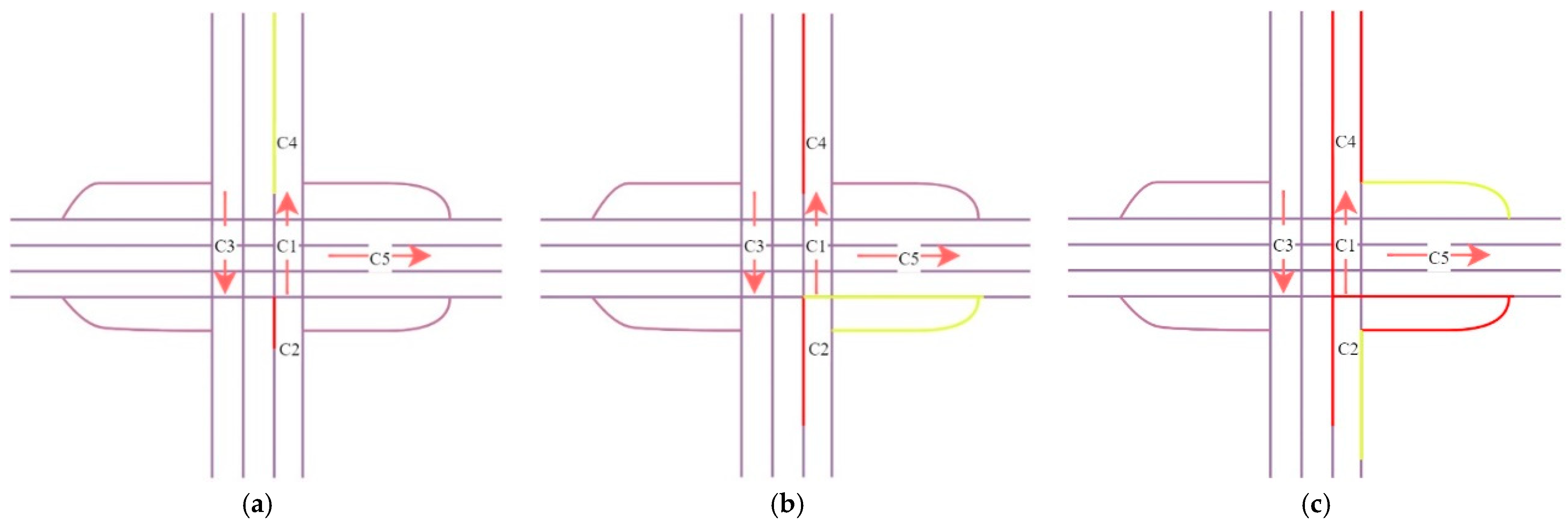
Figure 1, the main road connecting a city with its outskirts is depicted, with vehicles C1, C2, C3, C4, and C5 signifying the traffic flow situated on it. C1, C2, C4, and C5 travel from the city centre towards the outskirts, while C3 moves in the opposite direction. As time passes, during the evening hours, traffic congestion initiates at C1, as shown in
Figure 1a. Subsequently, other vehicles, such as C2, C4, and C5, are also affected by this congestion, as illustrated in
Figure 1b. Eventually, all vehicles connected to C1 experience heavy congestion, while C3 remains congestion-free, as depicted in
Figure 1c. These observations indicate that the spread of traffic situations is primarily influenced by the interconnectedness of road segments in the network structure, rather than by their spatial proximity.
Note: In above Figure, the arrows represent movement of vehicles in a particular lane, red lines represent the traffic congestion and green line represents the smooth passage or slip roads for traffic movement.
In sustainable smart cities, the efficient management of traffic is crucial to optimising transportation systems, reducing congestion, and minimising environmental impacts. Real-time estimation of traffic speed plays a vital role in achieving these goals. Traditional methods of traffic-speed estimation rely on sensors and data collected from fixed locations, which often have limitations in terms of coverage, accuracy, and real-time updates. To overcome these limitations, a Graph Neural Network (GNN)-based approach has emerged as a promising solution for real-time traffic-speed estimation in sustainable smart cities. GNNs are a type of deep-learning model specifically designed to analyse and process graph-structured data, where the nodes represent entities (such as intersections or road segments) and edges represent the relationships or connections between them. The GNN-based approach for traffic-speed estimation leverages the inherent graph structure of urban road networks to capture the spatial dependencies and temporal dynamics of traffic flow.
By considering the interdependencies between different road segments and their influence on each other, GNNs can learn complex patterns and make accurate predictions. In order to accurately predict the traffic speed, several studies on GNNs (Graph Neural Networks) [
8,
9] and GCNNs (Graph CNNs) [
10] have generated novel concepts. This is the inspiration behind this study, where the problem is formulated considering both input and output as a sequential graph. There are still some open research challenges that need to be addressed. The first challenge is how to extract important characteristics from intricate road networks in order to discover patterns or trends in the growth of traffic speeds. The second challenge is that the current research on GNNs only produces a single value and not a series of graphs when the network is fed sequential inputs. The third challenge is that the typical structure of sequence-to-sequence models (Seq2Seq) of the encoder and decoder techniques are inadequate for directly processing graph-structure data.
1.1. Research Contribution
In this study, a brand-new deep Graph Neural Network-based traffic-speed estimate model is suggested. The main contributions of this study are summarised as follows:
The structure and characteristics of road networks are taken into consideration by implementing DGNNs. The proposed technique trains a neural network for the accurate prediction of traffic flow using data from the entire road network.
The proposed approach is an extension of a DGNN that uses Gated Graph Attention Network (GGAN) blocks for the modification of inputs and outputs to sequential graphs.
Extensive experiments on real-world datasets show that the proposed model based on DGNNs predicts outcomes accurately. The suggested model’s validation and forecasting of traffic flow are put to the test against current state-of-the-art models.
1.2. Article Organisation
The rest of the article is structured as follows: A few relevant studies are discussed in
Section 2. The preliminaries are discussed in
Section 3, followed by a description of the proposed model in
Section 4. The experimental analysis and performance evaluation of the proposed model is presented in
Section 5. Last, the concluding remarks are presented in
Section 6, with some suggestions for future research.
3. Preliminaries
In this work, for developing a Graph Neural Network for an urban road network, consider a weighted directed graph G. The network is made up of N nodes with M edges, and this graph shows the connections between the primary node, an adjacency matrix A, and a weight matrix W.
Several factors need to be taken into account when converting a road network into a topology graph based on its physical structure in order to provide proper representation and prevent subpar prediction accuracy. The various considerations taken in this article, together with their consequences are as follows:
A limited range of node detectors: It becomes difficult to define the link connections in places with poor detector coverage. This indicates that other data sources or approaches should be taken into account throughout the graph generation process in order to correctly depict traffic flows and connections. The absence of node detectors in these locations can be partially made up for by integrating data from other sensor types or from sophisticated traffic monitoring systems.
Traffic direction and safety measures: Turning motions and safety measures cause traffic in different crossing lanes to flow in different directions. Investigating and taking into account the traffic direction data for each lane is needed in order to build an accurate directed graph. This indicates that in order to accurately represent actual traffic patterns, the graph needs include the precise traffic movements that are permitted or forbidden in certain lanes.
Correlations in space and pointless connections: In an urban road network, not all nearby roads exhibit robust spatial connections. Physical road network links alone may provide a large number of unnecessary connections, which would decrease forecast accuracy. The graph architecture should take into account how the traffic moves and how cars travel between various parts of the road network to handle this. It is important to consider proximity in space, where cars might likely reach nearby routes in close proximity. In order to build the highway network, researchers have also used node distances, demonstrating that the graph representation may be affected by both geographical closeness and real distance.
It is crucial to remember that static elements like distances and nearby relationships may fall short of adequately capturing the dynamic nature of traffic dynamics. The accuracy and efficiency of the graph representation can be improved by including real-time traffic data, such as traffic volumes, speeds, and congestion levels.
Problem Statement
In this article, we aim to learn a mapping function f that calculates the future traffic volumes y(t + 1) = x1(t + 1), x2(t + 1), …, xN(t + 1) given the historical traffic data of the road network with N detectors X(t) = x1(t), x2(t), …, xN(t) in the previous s time steps.
Then, we dissect the elements of the problem:
Traffic Volumes: The traffic volumes in the historical traffic statistics were gathered from N detectors at various time steps. The data for each detector is written as Xi(t) = xi(ts + 1), xi(ts + 2), …, xi(t), which indicates the traffic volumes seen at detector i in the preceding s time steps.
Specific Graph Structure: A graph G may be used to describe the road network, with the detectors acting as its nodes, and the edges signifying the connections or interactions between them. Different detectors’ spatial relationships are captured by the particular graph structure G.
Mapping Function f: The mapping function f forecasts the future traffic volumes y (t + 1) using the graph structure G and past traffic data X(t) as inputs.
The objective is to learn this mapping function f in order for it to accurately estimate future traffic volumes and capture the latent spatio-temporal correlations in the historical traffic data.
In order to anticipate future traffic volumes, the traffic-flow prediction problem makes use of previous traffic data, graph structure, and a mapping function. The aim is to uncover the hidden spatio-temporal dependencies in the data to make accurate predictions.
4. Proposed Methodology
This article analyses the different traffic-speed prediction methods along with proposing a real-time traffic-speed estimation methodology that can effectively combat the challenges of the present methods reported in the literature. The proposed methods are effective in terms of improved prediction accuracy as well as minimising the model errors. The major focus of real-time traffic-speed estimation is the observation of traffic speed utilising N different sensors, and the GNN-based deep-learning model is utilised for the analysis of mass traffic data [
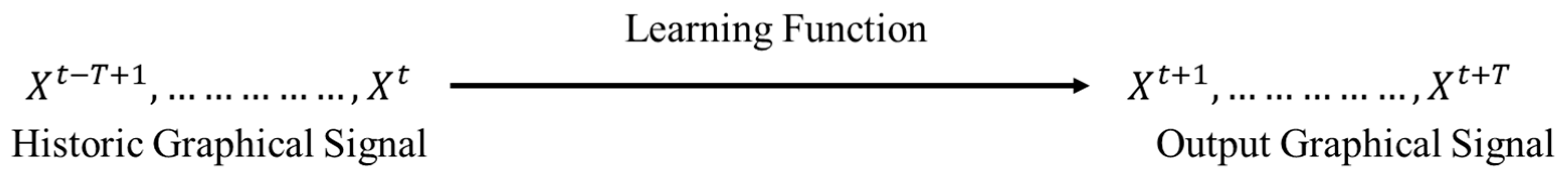
38]. The prediction of traffic signals is performed by the graph network; therefore, the relationship between N sensors is visualised using different GNNs. While expressing the graph of traffic speed as
, the graphical signal is expressed as
where the signal is observed over the time t. For the estimation of traffic speed, the challenge is solved by learning a function from the historic graphical signal in order to obtain the output future graphical signal. The detailed signal version is depicted in
Figure 2.
The input can be expressed in terms of two different feature domains. One is in terms of the spatial domain, where it is expressed as the collected features based on the basic parameters of traffic speed. However, in the temporal domain, this can be expressed as the conjunction of time-sequenced traffic-speed parameters. For defining the traffic speed, three different input parameters are considered, which are the flow of traffic, traffic density, and the speed of traffic vehicles. These are denoted as:
Flow of Traffic: The complete number of vehicles expressed in terms of their passage from a certain place in a specific time interval. It is expressed as Equation (1).
where
D is the density of traffic flow and
v is the velocity of traffic vehicles.
Traffic Density: This refers to the vehicle density at a particular date and is expressed as Equation (2).
Speed of Traffic vehicles: The speed of traffic vehicles is defined as the ratio of the road segment length to the average travel time for the vehicles to pass through a road segment. The expression for the average traffic vehicle speed is expressed as Equation (3).
where
is the length of the road section,
n is the vehicle number, and
is the speed of travel for the
ith vehicle.
4.1. Feature Analysis for Traffic-Speed Prediction
The analysis for traffic speed in this article is performed using Pearson’s correlation analysis for evaluating the quantitative periodicity of the traffic speed. A heatmap is utilised to evaluate the values obtained using the Pearson correlation analysis. This analysis provides the periodic characteristic of closeness in traffic-speed data. The Pearson coefficients are utilised to measure the degree of closeness through the correlation analysis [
39]. The Pearson coefficient (
PC) is computing between the future predictions (
F) and the historical data (
H). It is expressed as Equation (4).
In this equation,
TD represents the duration of the prediction, and the future predicted traffic speed is indicated by
F. The historical data
H is utilised for traffic-speed predictions. The mean values for both the historical and future predicted data values are represented by
and
, respectively. The value of
PC ranges between −1 and 1. A stronger positive correlation is indicated by values closer to 1, while
PC values closer to 0 indicate a weaker correlation. The complete description of strong and weak correlations are provided in
Table 2.
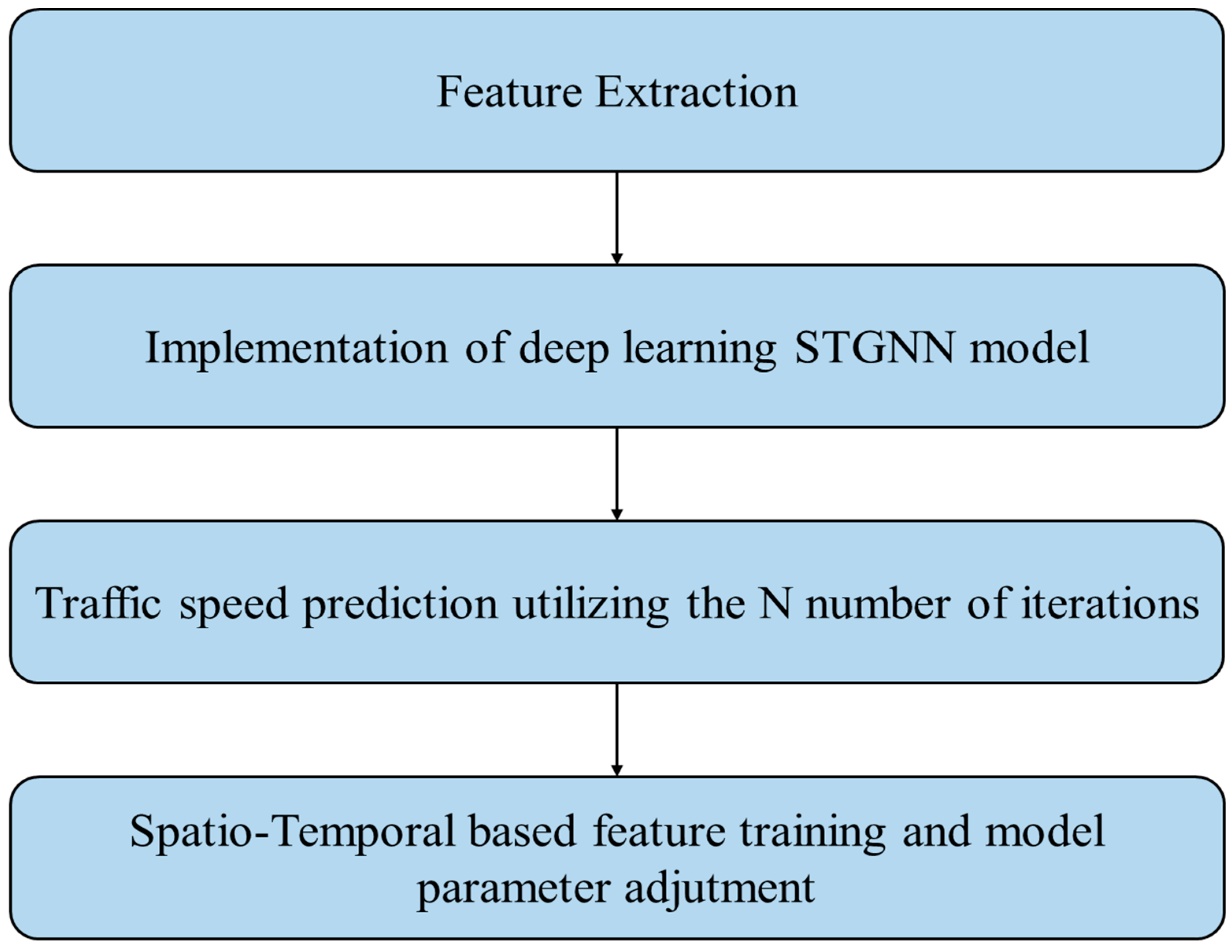
The outcomes obtained by the Pearson correlation analysis are utilised as the objective function for confirming the intermittent constituent module. It also verifies the applicability of the universal correctness of dataset selection. Furthermore, the second component of the proposed model framework utilises the multi-layered spatial–temporal graph analysis. This analysis is performed using the multi-layered Spatio-Temporal Graph Neural Network (STGNN). This neural network module has the capability of extracting the temporal as well as spatial characteristics for traffic-speed data prediction [
40]. The three main modules utilised in this article are depicted in
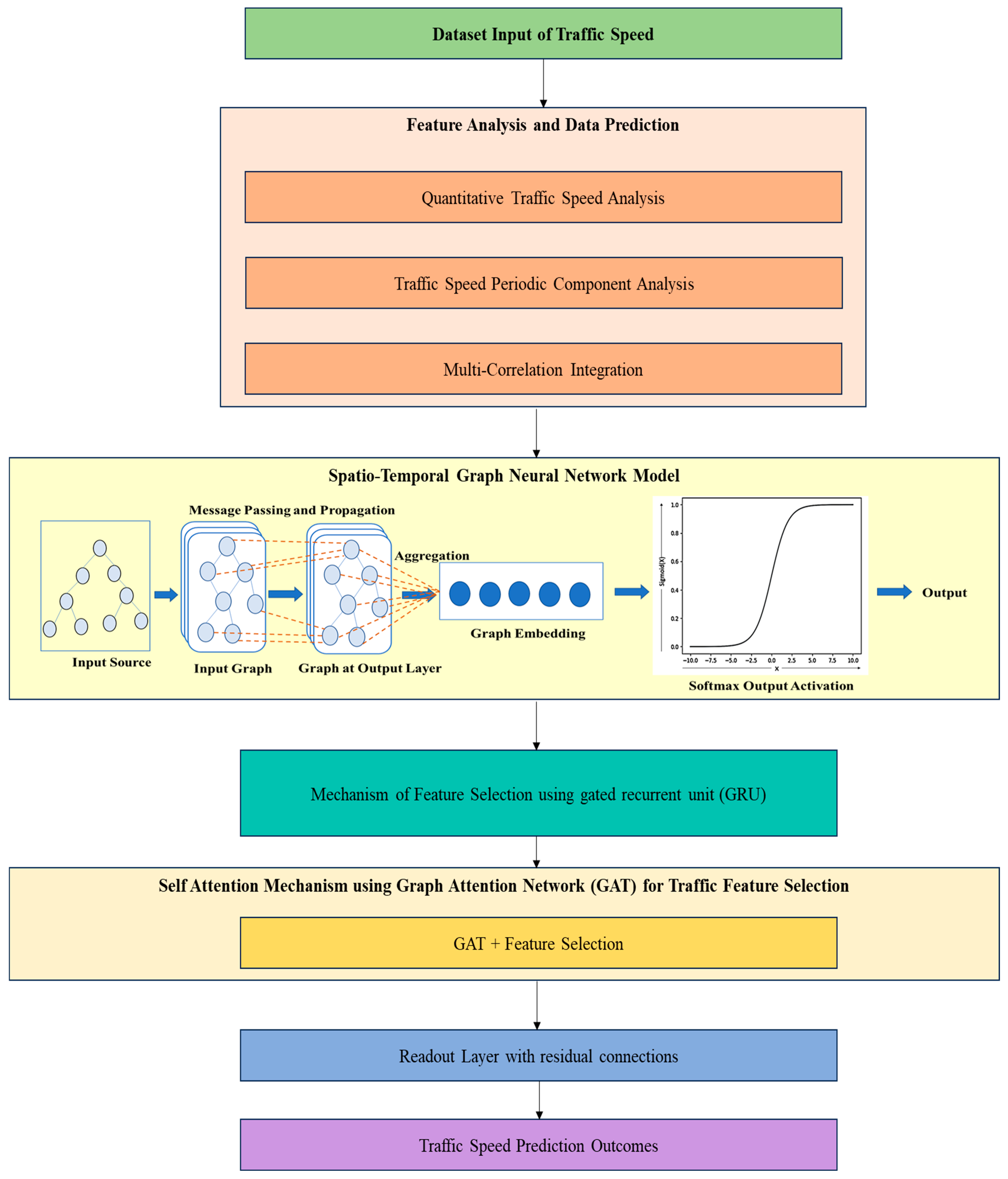
Figure 3.
The framework includes feature extraction in the first stage, followed by the aggregation of spatial features so as to provide the outcomes for the deep-learning model. The deep-learning STGNN model is utilised in the second stage of this article to obtain the extracted feature set for traffic-speed data utilisation. Furthermore, the final stage involves the traffic-speed prediction utilising the N number of iterations. The STGNN model completely learns the various spatial and temporal characteristics extracted from the features. The significantly reliable and high-dimensional feature information is utilised for the STGNN model. Furthermore, this model utilised the spatio-temporal-based feature training, and model parameters are adjusted through the forward proceeding of the model and the back propagation of the error values. This improves the accuracy as well as reliability of the proposed traffic-speed prediction framework.
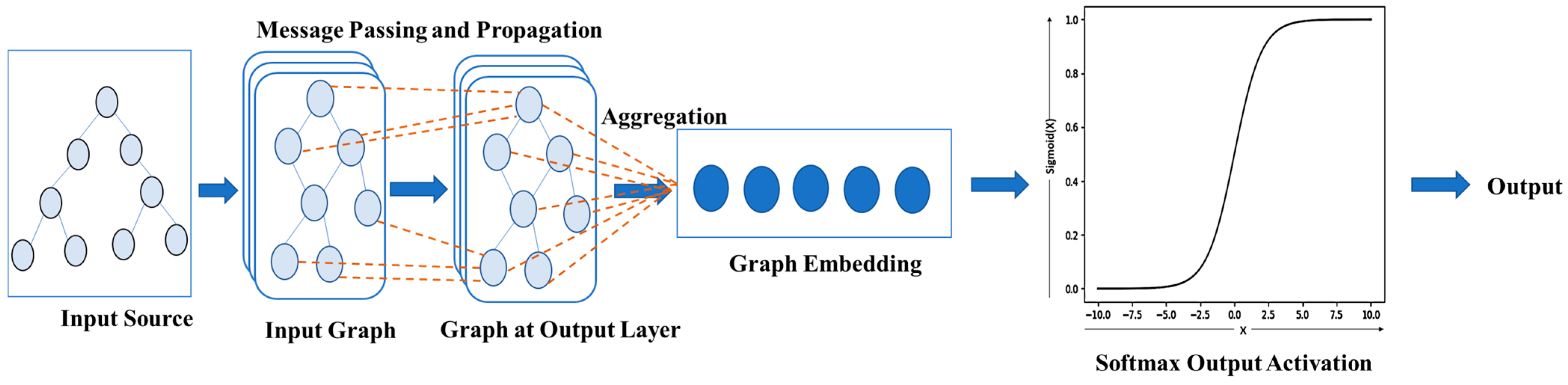
Furthermore, the key components of the STGNN-based approach consider various steps involved like the building graph representation, node and edge embeddings, message passing, and temporal dynamics involved in it, followed by prediction and evaluation.
Building Graph Representation: Building a graph representation of the road network is the initial stage in the GNN-based methodology. The connection between segments of a road is modelled as edges, and each piece of the road is represented as a node. The nodes or edges may also have other features, such as the length of the road, the posted speed limit, and past traffic information.
Node and Edge Embeddings: To capture the characteristics and connections found in the graph, GNNs need node and edge embeddings. Edge embeddings may depict the spatial relationships between linked segments, whereas node embeddings can store information about the features of individual road segments.
Message Passing: GNNs use a message-passing mechanism to collect and spread information throughout the graph. Nodes communicate with their neighbours throughout each iteration, updating their own representations in response to the messages they receive. GNNs may record both local and global dependencies inside the network thanks to this iterative approach.
Spatio-Temporal Dynamics: GNNs may be expanded to include spatio-temporal dynamics in order to perform real-time traffic-speed estimations. GNNs may learn patterns and trends over time by taking into account historical traffic data and the order of prior speed measurements, allowing precise forecasts of future traffic speeds.
Prediction and evaluation: The GNN model may be used to forecast real-time traffic speeds for various road segments in the smart city after being trained on historical data. Utilising suitable measures, such as mean squared error or mean absolute error, the model output may be assessed against ground-truth speed measurements.
The GNN-based approach for the real-time estimation of traffic speed offers improved accuracy by capturing the spatial dependencies and temporal dynamics within the road network. GNNs can provide more accurate and fine-grained predictions of traffic speed compared with traditional methods. GNNs are capable of processing data in real-time, enabling timely updates of traffic-speed estimations. This information can be used for dynamic route planning, congestion management, and for optimising traffic signal timings. These GNN-based approaches can be scaled to large road networks, making them suitable for implementation in sustainable smart cities with extensive transportation systems. The GNN framework can be modified to incorporate additional data sources such as weather conditions, event information, or sensor data from vehicles to enhance the accuracy of traffic-speed estimation. These applications of GNN-based approaches for real-time traffic-speed estimation aligns with the goals of sustainable smart cities, promoting efficient transportation, reducing congestion, and improving overall urban mobility. By leveraging the power of deep learning and graph analysis, these approaches contribute to building smarter, greener, and more sustainable cities.
4.2. Methodological Framework
The previous section provided an overview of the traffic-speed prediction analysis and identified the research gaps in the recent literature. The objective is to estimate the traffic speed in real-time using a GNN-based approach. This involves predicting the speed of vehicles at different locations in the city based on historical and current data. For this purpose, data collection is performed including the historical traffic-speed records, sensor data (e.g., from traffic cameras or GPS devices), road network information (e.g., road segments, intersections), and any additional contextual data (e.g., weather conditions, time of day). After data collection, handle any missing values and perform any necessary transformations or feature engineering. Convert the data into a suitable format for GNN-based models. Then, represent the network as a Spatio-Temporal Gated Graph Attention Network (STGGAN); here, the edges between the nodes define their connectedness based on the structure of the road network, while the nodes themselves represent road segments or intersections.
The STGGAN model contains a Gated Recurrent Unit (GRU) layer for capturing temporal correlations, a GAT layer with edge features for modelling spatial dependencies, an RNN-based gated module for assessing attention and significance, and a residual structure for increased training effectiveness. Combining both spatio-temporal data and graph structures, these elements allow the model to accurately estimate short-term traffic flow on urban road networks. For the purpose of predicting traffic flow on metropolitan road networks, the STGGAN (Spatio-Temporal Graph Attention Network) model is presented. To identify spatio-temporal relationships and enhance the model’s functionality, it includes a number of components. Using a GRU (Gated Recurrent Unit) layer, temporal correlations are captured. The model can learn temporal patterns in the data thanks to the GRU layer’s assistance in capturing dynamic variation features across past traffic conditions. The self-attention mechanism in the model adds edge characteristics for modelling spatial interactions. This feature increases the model’s capacity to capture spatial relationships between various sections by supplying prior knowledge about the characteristics of the road network. In order to assess the significance of various elements inside the multi-head attention mechanism, an RNN-based gated module is presented. During the prediction phase, this method enables the model to concentrate on pertinent information and to distribute attention efficiently. The STGGAN model adopts the residual readout layer structure, inspired by residual mapping, to hasten convergence and to capture minute changes. A residual structure increases the forward speed of information by allowing it to transcend many layers, allowing the model to efficiently optimise and capture the identity mapping.
Thus, the proposed STGGAN model combines a GRU layer, edge features, an RNN-based gated module, and a residual structure in contrast to the naïve GAT model. By collecting both the geographical and temporal linkages in traffic data, this improves the model’s capacity to derive spatio-temporal dependencies. The STGGAN model’s capacity to simulate the connections between various parts of the road network is improved by using edge features for a directed arc to better capture spatial interactions. A directed arc in a transportation network denotes a link or connection between two points or nodes. The model may include more details about the properties of the road segment that is represented by a directed arc by taking edge features into account. These edge features may comprise characteristics of the road segment, such as the kind of road, the speed limit, the amount of traffic, the state of the road, or any other pertinent data. The model may benefit from past knowledge of the road network’s properties by including edge features for a directed arc. The model may better comprehend the spatial interconnections and interactions between various road segments by taking these properties into account. When a model discovers, for instance, that some road types or situations often have a greater influence on traffic flow than others, it may adjust its forecasts appropriately. By merging the spatial and temporal components of the road network, edge characteristics in the STGGAN model result in a more thorough description of the road network. The GRU layer’s dynamic changes and the edge features’ spatial interactions are both taken into account in the model in order to properly predict short-term traffic flow on urban road networks in real-time. Therefore, using edge features for a directed arc in the STGGAN model facilitates the incorporation of spatial data and improves the model’s capacity to capture the intricate relationships between various parts of the road network, resulting in more precise traffic-flow predictions in sustainable smart cities.
For defining the Spatio-Temporal Gated Graph Attention Network (STGGAN) architecture, use the following steps.
Define the node features: assign initial features to each node, such as historical traffic-speed values or contextual information.
Define the edge features: compute edge features based on the relationship between nodes, such as distance or road connectivity.
Initialise node and edge representations: assign initial representations to nodes and edges.
Gating Mechanism: Introduce a gating mechanism to control the flow of information in the network. This can be achieved by using Gated Recurrent Units (GRUs) or other gating mechanisms.
Attention Mechanism: Implement a graph attention mechanism to capture the rank of neighbouring nodes for each node’s representation. This can be performed using attention coefficients that determine the relevance of neighbouring nodes during message passing.
Furthermore, model training is performed, which involves splitting data into training, validation, and testing sets. Initialise the model and then train it by using the training data to optimise it to minimise the prediction error. Furthermore, tune hyperparameters and monitor the model’s performance on the validation set to prevent overfitting. For real-time estimation, the trained network model is continuously updated for the graph representation and by feeding the new data into the STGGAN model to make predictions for traffic speed at different locations and updating the predictions as new data becomes available. Also, the model’s performance is assessed using appropriate evaluation metrics, such as mean absolute error or root mean square error. Compare the proposed approach with baseline methods or other relevant approaches. For the integration of the STGGAN-based traffic-speed estimation model with other smart city systems, such as traffic management systems or intelligent transportation systems, enable real-time monitoring and decision making based on the estimated traffic speeds. The architecture of the proposed STGGAN-based network designed for this research work is depicted in
Figure 4.
The proposed framework depicts the traffic speed for overcoming the shortcomings of the existing models. The interoperability of the input data is also improved along with the improvement in the learning ability of the deep-learned model for higher-order correlation analysis [
41]. Also, the proposed model is effectual in extracting the dynamic association between the traffic structure networks and the nodes. The proposed model framework is depicted in
Figure 5.
The proposed model comprises three different modules. The initial component is responsible for feature analysis as well as the periodic prediction of the data after fusion. The correlation analysis is performed for outputting the characteristic data determined after the feature analysis. Furthermore, the second component of the proposed framework is a convolution analysis based on the spatial–temporal Graph Neural Network. For the convolution analysis, this work utilises a multi-layered Graph Neural Network model so as to obtain a higher dimensionality in terms of the spatio-temporal feature processing obtained from the first component stage [
42]. The feature-selection-stage mechanism is introduced in the third component of the proposed model in order to improve the feature reliability of the extracted set of features for traffic-speed data.
4.3. Spatial Dependency
In order to anticipate traffic flow on urban road networks, knowledge of spatial relationships is essential. The Graph Attention Network (GAT) is used in this portion to capture these spatial relationships. The GAT has shown success in a variety of tasks, including recommendation systems and computer vision. The GAT offers a number of benefits over the popular Graph Neural Network (GNN) model for predicting traffic flow:
Weight Allocation: The GAT can handle directed graphs and may give different weights to various neighbours, which is useful for metropolitan road networks with direction-specific traffic flows.
Node characteristics: Rather than the graph structure itself, model parameters in GAT are tied to each node’s characteristics. The GAT may be used for inductive learning tasks thanks to this trait, which allows the model created for one set of road networks to be used to forecast traffic conditions on other road networks.
For the purpose of defining the GAT, we refer to the input characteristics of node
i at layer
l as
hil, where
hil denotes the input’s prior traffic states, or
Xti. The following is the GAT formulation indicated in Equations (5)–(7):
where
is the learnable weight matrix;
where
is a single-layer feed-forward network; and
The urban road network is transformed into a weighted directed graph for the road-network transformation method. Edge characteristics are disregarded in the aforementioned GAT layer as previous information to enhance the computation of attention weights in order to take use of the edge features. As a result, to optimise the process of computing the attention weights, we add the edge weights
E of the created weighted directed graph as prior knowledge. Additionally, including edge features into the GAT layer helps to lessen the effects of unused connections brought on by mistakes during construction. Thus, the softmax function is indication in Equation (8).
where
is the edge weight.
4.4. Temporal Dependency
Given that they represent the time-varying properties of network flow, temporal dependencies are essential for effectively forecasting future traffic states. Instead of relying only on a straightforward linear transformation in this work, we suggest using the Gated Recurrent Unit (GRU) to properly capture these temporal connections.
A linear transformation is employed to convert the lower-level characteristics into a high-dimensional space. However, as the input characteristics are essentially time-series data reflecting prior traffic conditions, this technique falls short of thoroughly examining the temporal evolution of the input features. We make use of GRU, a popular Recurrent Neural Network (RNN) variation recognised for its capacity to represent sequential input, to overcome this constraint.
Two essential parts make up a GRU block: a reset gate (
rt) and an update gate (
ut). The update gate aids in capturing long-term dependencies in the time series, while the reset gate is in charge of eliminating old data that is unrelated to future states. The GRU layer may be stated as Equations (9) and (10) for an input feature
it:
where
W is the weight matrix for reset gate and
; and
where
W is the weight matrix for update gate and
.
4.5. Spatio-Temporal Prediction Model Framework
For the purpose of predicting short-term traffic flow on urban road networks, the STGGAN (Spatio-Temporal Graph Attention Network) model is the output. A feature analysis and data prediction layer, a Gated Recurrent Unit (GRU) layer, a feature selection layer, and a GAT (Graph Attention Network)-based self-attention mechanism make up its four primary parts. The model seeks to capture both the geographical relationships between various road network segments and the temporal correlations in historical traffic data.
The feature analysis and data prediction layer, the initial element, is used to enhance the model’s capability of detecting temporal correlations. A Gated Recurrent Unit (GRU) layer aids in identifying sequential patterns in the data. Next, the GAT (Graph Attention Network)-based Graph Neural Network (GNN) model is enhanced using edge characteristics. The GAT is a Graph Neural Network design that can simulate the connections between various graph nodes. The Spatio-Temporal STGGAN model improves the spatial interdependence between various road network segments by including edge features, taking into account both traffic levels and the properties of the individual road segments. The value of various heads in the multi-head attention mechanism is assessed using the Recurrent Neural Network (RNN)-based gated module. When producing predictions, the model’s attention processes enable it to concentrate on pertinent portions of the data. Based on the input data, the gated module assists in dynamically allocating priority to various attention heads, enhancing the model’s capacity to pay attention to pertinent information.
Additionally, a readout layer with residual connections is adopted by the STGGAN model. Residual connections speed up training and increase convergence efficiency by allowing the model to learn from discrepancies between anticipated and actual values. This structure aids the model’s efficient learning and gradient propagation during training.
The algorithm for the Spatio-Temporal Graph Neural Network (STGNN) model uses a Gated Graph Attention Network-based STGGAN approach for the real-time estimation of traffic speed in sustainable smart cities. The goal is to predict the speed of vehicles at different locations in the city using historical and current data, taking into account the graph structure of the road network. The algorithm for GNN modelling is indicated as Algorithm 1:
| Algorithm 1: Spatio-Temporal Gated Graph Attention Network (STGGAN) |
Input:
X: Node features (node_count × feature_dim)
A: Edge features (node_count × node_count × feature_dim)
Parameters:
K: Number of attention heads
hidden_dim: Hidden dimension
output_dim: Output dimension
Initialise weight matrices: W_node (feature_dim×hidden_dim), W_edge (feature_dim× hidden_dim),
W_att (hidden_dim×hidden_dim) for each attention head, and W_out (K ×hidden_dim×output_dim)
Initialisation:
H = zeros(node_count, hidden_dim) # Node representations
E = zeros(node_count, node_count, hidden_dim) # Edge representations |
Node representation computation:
for k in range(K): # Attention heads
for i in range(node_count): # Nodes
h = GatingMechanism(H[i], X[i])
H[i] = h
Edge representation computation:
for k in range(K): # Attention heads
for i in range(node_count): # Source nodes
for j in range(node_count): # Destination nodes
e = LeakyReLU(H[i] * W_edge + H[j] * W_edge)
E[i, j] = e
Attention mechanism:
for k in range(K): # Attention heads
H = AttentionMechanism(H, E)
Output computation:
output = softmax(H * W_out)
return output
Function GatingMechanism(h, x):
# Gated Recurrent Unit (GRU) for gating mechanism
r = sigmoid(W_r * x + U_r * h)
z = sigmoid(W_z * x + U_z * h)
h_hat = tanh(W_h * x + U_h * (r * h))
h_new = (1 − z) * h + z * h_hat
return h_new
Function AttentionMechanism(h, adj):
# Graph attention mechanism
e = LeakyReLU(Attention(h * W_att, h * W_att))
alpha = softmax(e)
h_new = sum(alpha * h)
return h_new |
Here, the activation functions (e.g., sigmoid, tanh, LeakyReLU, softmax) and the weight matrices (e.g., W_node, W_edge, W_att, W_out) are assumed to be defined and initialised appropriately. The GatingMechanism and AttentionMechanism functions are defined separately to capture the specific computations involved in those steps.
This work provides an effective analysis of the data with traditional models. The proposed model is better compared with the traditional models in terms of data quality as well as input reliability. The system scalability is also improved in this proposed model as the calculation process is simplified and the connections are enhanced between different components. Thus, the proposed model is improved in terms of interpretability and accuracy.
5. Results and Analysis
The experimental analysis of the proposed STGNN-based STGGAN approach for real-time traffic-speed estimation while implementing it for smart cities was performed in this article using two different actual traffic datasets. The datasets utilised in this article are the PeMSD4 [
43,
44] and PeMSD8 [
43,
44] datasets, which comprise a varying number of samples and are sampled using a different number of sensors. The PeMSD4 dataset was acquired using 307 sensors which resulted in a total of 16,992 sample outcomes; however, the PeMSD8 dataset was acquired using 170 sensors and resulted in 17,856 sample sets. Feature details of the two datasets involved in this study are depicted in
Table 3.
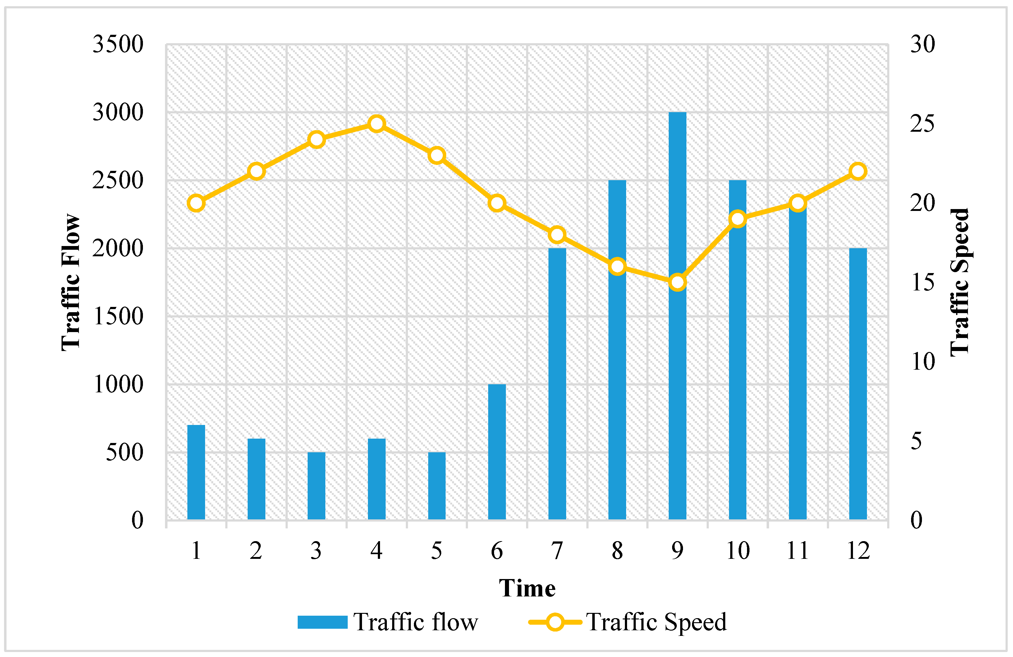
A measure of traffic flow and traffic speed for a density of approx. 500 vehicles per kilometre is depicted in
Figure 6. Based on the traffic flow and traffic speed indicated in
Figure 6, further measures were computed in terms of prediction accuracy (PA), mean square error (MSE), root mean square error (RMSE), mean absolute error (MAE), and mean absolute percentage error (MAPE).
For accurate prediction using the proposed STGNN-based STGGAN approach, the network performance was tested for its prediction accuracy which was computed in terms of True Positive (TP), True Negative (TN), False Positive (FP), and False Negative (FN) values obtained for both the PeMSD4 and PEMSD8 datasets. TP refers to the situation when the STGNN correctly predicts a positive outcome. In the case of traffic-speed estimation, it means that the STGNN accurately predicts a high traffic speed when the actual speed is indeed high. It represents the number of correctly identified high-traffic-speed instances. TN occurs when the GNN correctly predicts a negative outcome. In traffic-speed estimation, it means that the STGNN accurately predicts a low traffic speed when the actual speed is indeed low. TN represents the number of correctly identified low-traffic-speed instances. An FP happens when the STGNN incorrectly predicts a positive outcome. In the context of traffic-speed estimation, it means that the STGNN predicts a high traffic speed when the actual speed is low. FP represents the number of instances where the STGNN wrongly identifies high traffic speed. FN occurs when the STGNN incorrectly predicts a negative outcome. In the case of traffic-speed estimation, it means that the GNN predicts a low traffic speed when the actual speed is high. FN represents the number of instances where the GNN fails to identify high traffic speed. These definitions are based on the concept of binary classification, where the task is to categorise instances into two classes: high traffic speed and low traffic speed. The GNN is trained to predict the traffic speed based on the input graph data, and TP, TN, FP, and FN are computed by comparing the GNN’s predictions with the actual traffic-speed labels. By analysing the values of TP, TN, FP, and FN, various evaluation metrics can be computed to assess the performance of the GNN model, and these metrics provide insights into the model’s ability to correctly identify high and low traffic speeds, which are crucial for real-time traffic-speed estimation in sustainable smart cities.
This section presents a comparative analysis of the proposed STGNN-based STGGAN approach with some standard baseline models in order to assess the system’s performance. Furthermore, a vast comparative study was conducted using various statistical, analytical, machine-learning- and deep-learning-based approaches. The different evaluation criteria used in this article are PA, MSE, RMSE, MAE and MAPE.
The formulas for all the evaluation indicators are provided in Equations (11)–(15).
where
is the true value obtained,
is the predicted value of the sample outcome, and
is the total sample number.
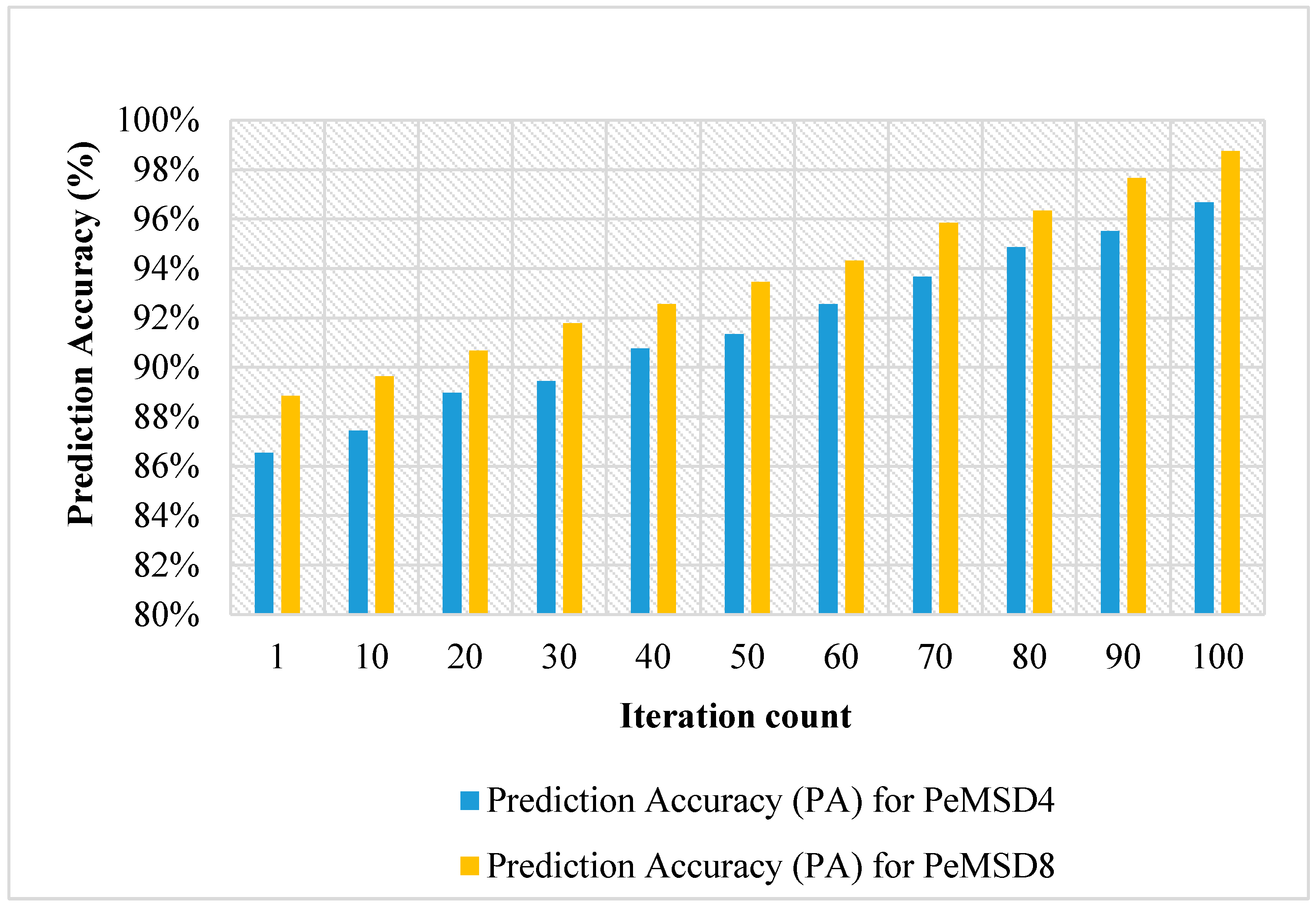
Furthermore, in this section, the impact of traffic speed at varying spatio-temporal locations is demonstrated and discussed using the model prediction accuracy for both PeMSD4 and PEMSD8 datasets. The computed prediction accuracy is shown in
Figure 7.
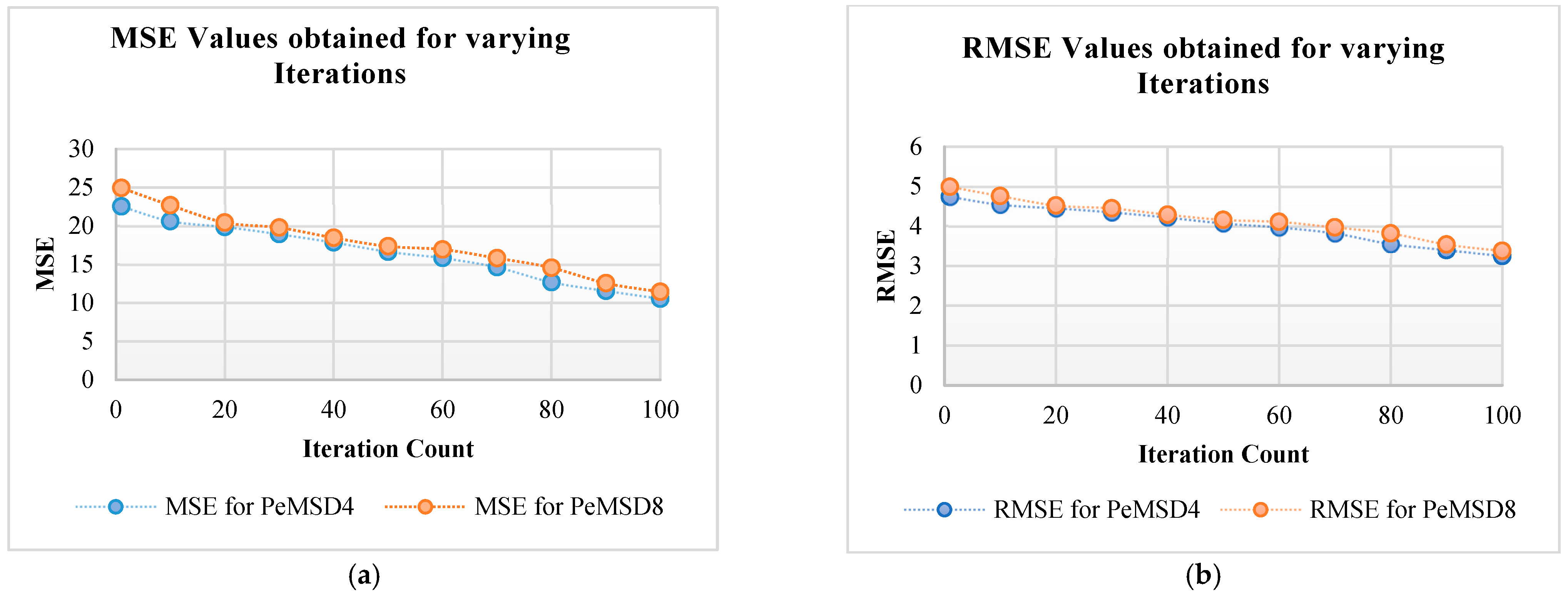
Figure 7 shows that the proposed STGGAN model is capable of improving the accuracy of traffic-speed predictions. As the number of iterations increased from 1 to 100, the accuracy of predictions for both the PeMSD4 and PEMSD8 datasets improved steadily. The accuracy values for PeMSD4 increased from 86.54% to 96.67%, and those for PEMSD8 increased from 88.85% to 98.75%. The proposed STGGAN model demonstrates accurate prediction abilities for light to moderate traffic flow. Consistently high prediction accuracy for these traffic volumes indicates the model’s ability to accurately predict traffic speed under such conditions. Furthermore, the error computation for the proposed STGGAN method was performed in terms of MSE and RMSE, which is revealed in
Figure 8a,b.
The MSE values observed from
Figure 8a shows that the error value reduces with an increasing iteration count, and it is still decreasing at a significant rate at the 100th iteration count. For the PEMSD4 dataset, an MSE value of 22.54 was observed for the 1st iteration, and this continued decreasing until an MSE value of 10.54 was obtained for the 100th iteration count. Similarly, for the PEMSD8 dataset, an MSE value of 24.95 was observed for the 1st iteration, which continued reducing until an MSE value of 11.43 was obtained for the 100th iteration count. The observations made from
Figure 8b reveal that the RMSE error values gradually reduce with the increase in the iteration count from 1 to 100. An RMSE value of 4.54 was observed for the 1st iteration which continued decreasing until reaching an RMSE value of 3.25 for the 100th iteration count for the PEMSD4 dataset. Similarly, for the PEMSD8 dataset, an RMSE value of 4.99 was observed for the 1st iteration which continued decreasing until an MSE value of 3.38 was obtained for the 100th iteration count. As the iteration count increases from 1 to 100, the mean squared error (MSE), root mean squared error (RMSE), mean absolute error (MAE), and mean absolute percentage error (MAPE) values decrease progressively. With increased iterations, the proposed STGGAN model obtains greater accuracy in predicting traffic speed, as indicated by this decrease.
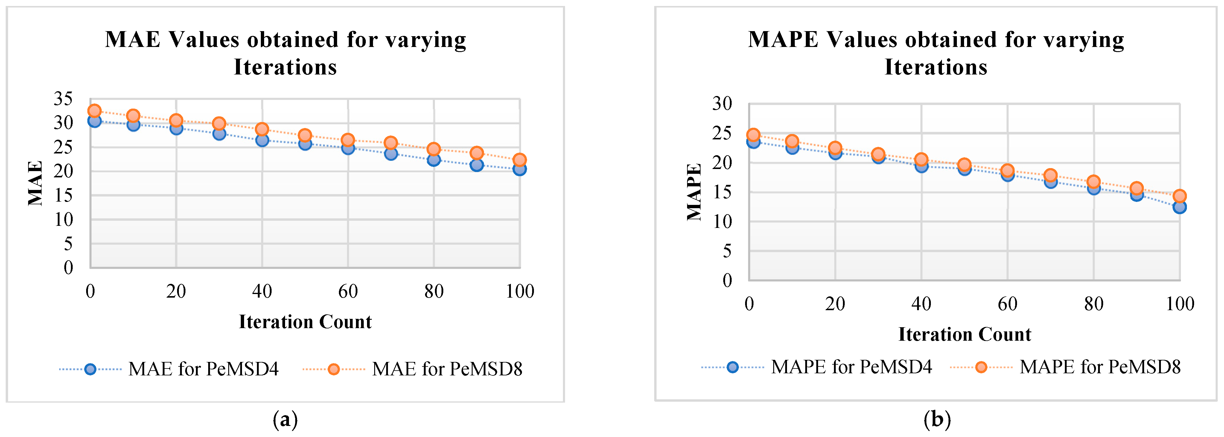
Figure 9a,b depict the MAE and MAPE values observed for the PeMSD4 and PEMSD8 datasets, respectively. In
Figure 9a, MAE values are observed from the 1st to the 100th iteration count. For the PEMSD4 dataset, an MAE value of 30.45 was observed for the 1st iteration which reduced to an MAE value of 20.45 for the 100th iteration count. Similarly, for the PEMSD8 dataset, an MAE value of 32.48 was observed for the 1st iteration which continued decreasing to 22.34 for the 100th iteration count. The observed computation reveals that the MAE value decreases with the increasing iteration count, and it decreases to a significantly much lower value at the 100th iteration.
Figure 9b depicts the MAPE values for the PeMSD4 and PEMSD8 datasets. Utilising the PEMSD4 datasets, an MAPE value of 22.56 was observed for the 1st iteration, which minimised to 12.45 for the 100th iteration. For the PEMSD8 dataset, an MAPE value of 24.69 was observed for the 1st iteration while being minimised to 14.32 for the 100th iteration count. This reveals that MAPE error values are gradually reduced with the increasing iteration count. There are certain baseline models which are analysed in this work for the validation analysis of the proposed STGGAN approach. Several baseline models, including Genetic Algorithm (GA), Particle Swarm Optimisation (PSO), Artificial Neural Network (ANN), Traditional Convolutional Neural Network (CNN), and Multi-Layered Graph Neural Network (STGNN), are contrasted with the proposed STGGAN model. The comparison consists of prediction error, execution time, and evaluation metrics, including MSE, RMSE, MAE, and MAPE.
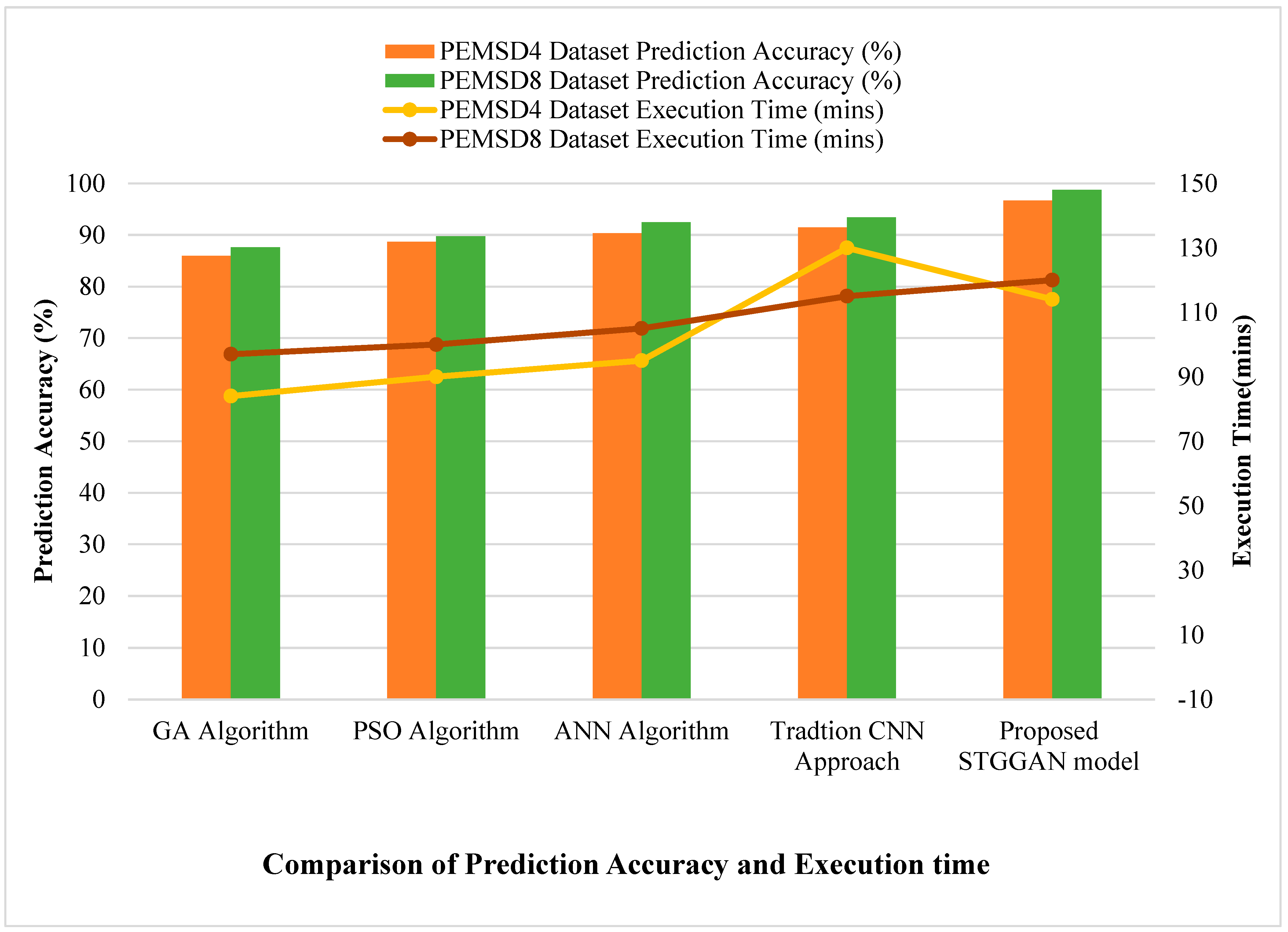
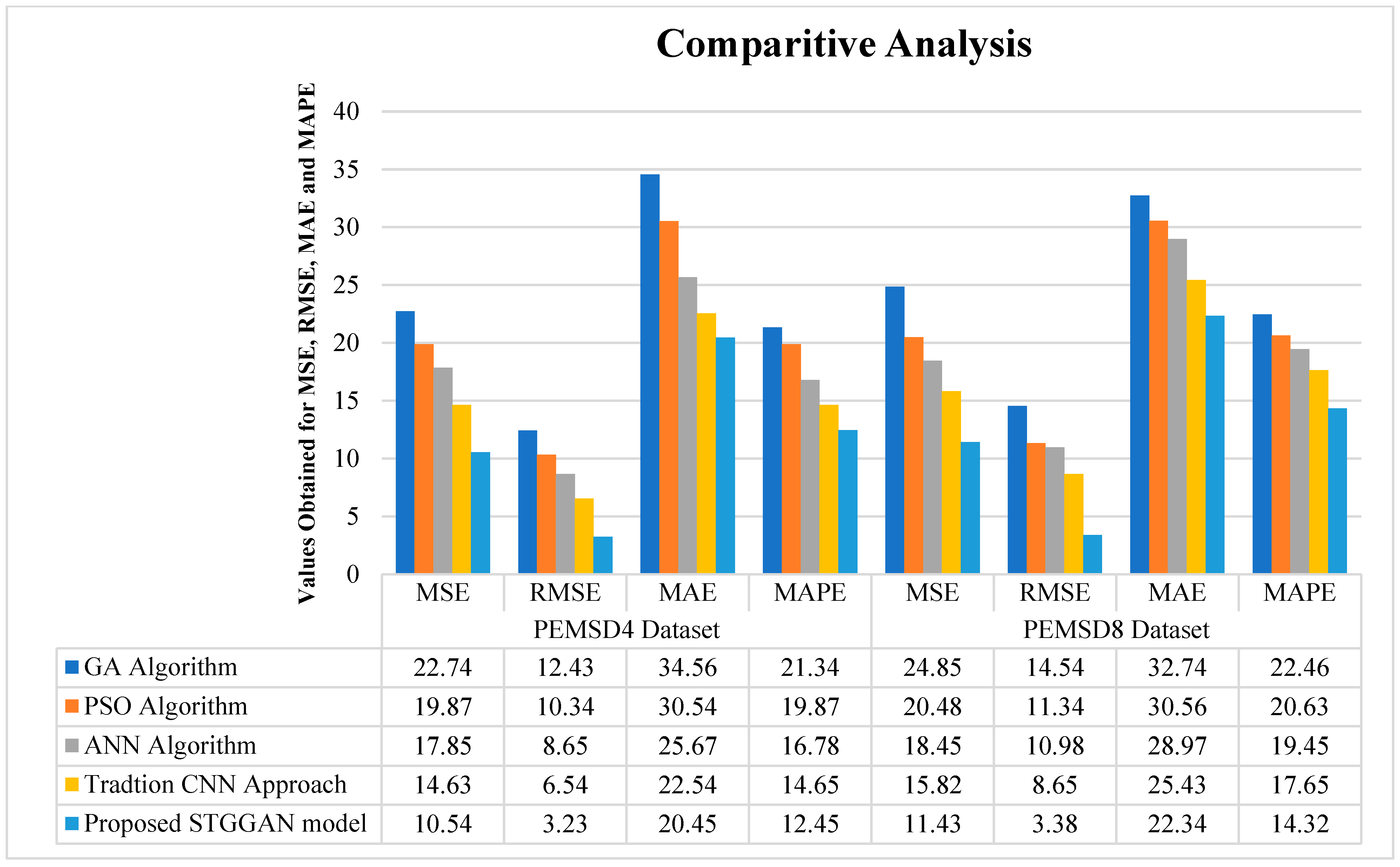
The comparison of prediction error and execution time is provided in
Figure 10 and of MSE, RMSE, MAE and MAPE errors in
Figure 11.
The comparative analysis demonstrates that the proposed STGGAN model obtains greater prediction accuracy than other algorithms for both the PeMSD4 and PeMSD8 datasets. For PeMSD4, the proposed STGGAN model achieves a prediction accuracy of 96.67%, outperforming the GA algorithm (85.94%), the PSO algorithm (88.67%), the ANN algorithm (90.34%), and the conventional CNN approach (91.45%). Similarly, for PeMSD8, the proposed STGGAN model achieves a prediction accuracy of 98.75%, outperforming the GA algorithm (87.59%), the PSO algorithm (89.74%), the ANN algorithm (92.45%), and the conventional CNN approach (93.45%).
According to the execution time analysis, the proposed STGGAN method required 114 min for the PeMSD4 dataset and 120 min for the PeMSD8 dataset. These values indicate the computational efficacy of the proposed STGGAN model, even though the execution time is not explicitly compared with other algorithms.
The comparative analysis of the mean squared error (MSE), root mean squared error (RMSE), mean absolute error (MAE), and mean absolute percentage error (MAPE) for both datasets demonstrates that the proposed STGGAN model achieves better values than the other algorithms. Lower MSE, RMSE, MAE, and MAPE values indicate greater precision and accuracy in traffic-speed prediction. The effectiveness of the proposed STGGAN model is further supported by the fact that all these metrics exhibited significant enhancements. The proposed STGGAN method exploits the spatial and temporal dependencies in the data by utilising the characteristics of a Graph Neural Network. This incorporation enables the model to capture and exploit the intricate relationships and patterns present in traffic data, which contributes to its enhanced performance. The technical observations emphasise the practicability and viability of the proposed STGGAN method. Compared with other algorithms, the model yields more accurate predictions and enhanced evaluation metrics, demonstrating its reliability. These results validate the efficacy and applicability of the proposed STGGAN model for predicting traffic speed.
In terms of prediction accuracy, evaluation metrics, and usability, the proposed STGGAN model outperforms other algorithms, according to the technical observations. Its enhanced performance is a result of the incorporation of Graph Neural Network characteristics, making it a promising approach for traffic-speed prediction tasks.
The Spatio-Temporal Traffic Prediction Model (STGGAN) framework has a number of significant advantages over other alternative methods for traffic prediction utilising Graph Neural Networks (GNN) reported in the literature [
25,
26,
27]. A few of the significant advantages are listed below:
Comprehensive Integration: The STGGAN framework incorporates both spatio-temporal data and graph structures, enabling an all-encompassing approach to traffic prediction. This comprehensive integration enables the model to encompass the complex relationships between spatial and temporal factors, resulting in more accurate forecasts.
Capturing Temporal Correlations: The STGGAN framework includes a Gated Recurrent Unit (GRU) layer that effectively captures temporal correlations in the traffic data. By taking into account dynamic variations across prior traffic conditions, the model can learn and adapt to temporal patterns, thereby improving its accuracy of prediction.
Modelling Spatial Dependencies: With the incorporation of a Graph Attention Network (GAT) layer with edge characteristics, the STGGAN framework excels at modelling spatial dependencies. This feature allows the model to utilise prior knowledge about the road network, such as road types, speed limits, and other characteristics, in order to capture the complex interactions between various road sections.
Attention Evaluation: The STGGAN framework employs an RNN-based gated module to evaluate the attention and significance of various elements within the multi-head attention mechanism. This mechanism enables the model to focus on pertinent information and effectively distribute attention, thereby enhancing its overall prediction performance.
Residual Structure: Motivated by residual mapping, the readout layer of the STGGAN framework employs a residual structure. This structure enables faster convergence and the capture of minute changes in the traffic data, thereby enhancing the model’s optimisation capabilities and allowing identity mapping to be effectively captured.
Real-Time Estimation: The STGGAN framework’s ability to estimate short-term traffic flow in real time is one of its primary strengths. By integrating spatio-temporal data and graph structures, the model is able to provide accurate predictions in a timely manner, thereby facilitating smart city traffic management and decision making.
Thus, by integrating geographical and temporal data, using previous data, adjusting to real-time changes, and offering scalability and interpretability, the Spatio-Temporal Traffic Prediction Model framework offers a holistic approach to traffic prediction. It is a potential option for precise and effective traffic forecasting using GNNs because of these benefits. These benefits distinguish the STGGAN framework from alternative approaches and demonstrate its efficacy in addressing the challenges of traffic prediction. The comprehensive integration of spatio-temporal data and graph structures, as well as the incorporation of temporal correlations, spatial dependencies, attention assessment, and residual structure, all contribute to the superior real-time traffic flow estimation performance of the STGGAN model.


 ,
, 


