Assessing Coastal Land-Use and Land-Cover Change Dynamics Using Geospatial Techniques

Abstract

Geospatial techniques can be used to assess the dynamic conditions of coastal land use and land cover in order to make informed decisions about future management strategies for sustainable development through a combination of remote sensing data with field observations of shoreline characteristics along coastlines worldwide. Geospatial techniques offer an invaluable method for analyzing complex coastal systems at multiple scales. The coastal land use and land cover from the Subarnarekha (Orissa) to the Rasulpur estuaries (West Bengal) along the Bay of Bengal are dynamically modified by a complex interaction between land and sea. This is due to various dominating factors of physical and anthropogenic activities, which cause changes in the landscape. The main objective of this study was to identify the periodical transformation and changes in land-use/land-cover (LULC) features by the USGS-LULC classification method using a maximum-likelihood classifier (MLC) algorithm and satellite images for the period 1975–2018. The entire study area was divided into three ‘littoral zones’ (LZs). This will help in understanding how LULC has changed over time, as well as providing insight into human activities impacting on coastal environments. This study focused on five features selected for LULC classification, namely, built-up, vegetation, soil, sand and shallow-water areas. The purpose of this study was to investigate human encroachment near shore areas as well as the transformation of soil and sand into built-up areas over a 43-year period from 1975 to 2018 using geospatial techniques. To estimate the changes in the areas, a geodatabase was prepared for each LULC feature. Finally, statistical analysis was performed on all available datasets, which allowed the researchers to identify trends in land-cover change from 1975–2018 within each category, such as increasing deforestation and urbanization rates due to increased population growth. The results of the study show the expansion of shallow-water areas, which is one of the major factors influencing coastal erosion. Maximum shallow-water-level enhancement was observed in LZ I and LZ II. In LZ I, shallow water increased from 1 km² to 4.55 km². In LZ II, the initial 1.7 km² shallow-water area increased to 13.56 km², meaning an increase of 11.86 km² in shallow-water zones. A positive change was noticed in vegetation area, which increased from 2.82% (4.13 km²) to 15.46% (22.07 km²). Accuracy assessment was applied for all classified images, and more than 85% accuracy was considered for the overall accuracy assessment. Finally, Kappa coefficient statistics were adopted to complete the accuracy analysis, and 80% or more than 80% accuracy was obtained for all classified images. This information can also help inform policy makers about potential environmental impacts associated with certain activities, such as coastal development and agricultural expansion, so that appropriate steps can be taken towards mitigating these impacts before it is too late.

1. Introduction

The present study area (Subarnarekha to Rasulpur estuary) has experienced remarkable modification in land-use and land-cover features due to the increase in the water level and the growth of unplanned urbanization over four decades [1]. The coastal area between the Rasulpur to the Subarnarekha estuaries in the states of West Bengal and Orissa, India, has been facing acute environmental disruption in the form of loss of sediment, shoreline shifting, seawater intrusion, loss of landforms due to quickened changes in land use/land cover by rapid climatic changes, human encroachment, sea-level rise and growth of commercial activities [1]. The East Coast of India, especially the Bay of Bengal, is very active, being subject to ocean-related shocks, and is a more inundated region than India’s West Coast. The East Coast of India is experiencing a similar situation, although there are quantitative differences from area to area. Deltaic formation, human activities, sediment supply, offshore bar formation and basement faulting have also been affected by the local sea-level rise and global warming over three decades in this zone. The coastal belt of Orissa and West Bengal is especially vulnerable to the effects of climate change due to its mud- and sand-based composition. This region is more susceptible than other parts of India’s coast, as rising sea levels can cause severe erosion, flooding, loss of agricultural land, destruction of infrastructure and displacement of those living in low-lying areas. In addition, there is an increased risk from natural disasters, such as cyclones, which can devastate entire coastlines if they are not adequately prepared for beforehand through proper planning initiatives put into place by policy makers. The land-use/land-cover transformation due to several environmental and socio-economic phenomena is affecting the natural conditions of local habitats along the coastal zone in space and time. Coastal zones require a huge amount of spatial research to assess their geomorphic changes [2]. Land use is the cumulative output of the relation between natural and manmade processes. To execute some planning and management in coastal areas, land-use and land-cover (LULC) distribution analysis is the most essential tool [3]. The existing land use and land cover is modified by the rapid growth of urbanization and extensive human encroachment in coastal areas [4,5,6,7,8]. Due to various storm surges, tsunamis and global warming, the water level is increasing day by day. Low-lying coastal areas are inundated by the global sea-level rise. Due to this rise, coastal habitats and many developments have been damaged in coastal areas. In the assessment of coastal vulnerability, the coastal land-use/land-cover area is extremely transformed due to several coastal parameters, such as waves, tides, wind, saltwater intrusion, storm surge, sea-level rise and human interference [2,9,10,11,12]. Growth of population and various climatic disturbances put pressure on land use/land cover, which causes massive environmental effects in terms of shoreline change, vegetation cover, saltwater intrusion, water degradation, sand-dune loss, degradation of biodiversity and soil deterioration, all of which have been observed along coastal zones [3,13,14,15].

It has been reported by the UNPD [16] that coastal populations have been putting pressure on coastal areas during the past 40 years and that this will increase in the same way in the next 40 years. Extreme growth of population leads to a rapid pace of land-cover change due to the expansion of various settlement infrastructures [17]. Now, these changes have been putting major pressure on existing coastal populations and ecosystems in recent decades [6,18,19]. These kinds of negative impacts increase the vulnerability of coastal regions and people to economic, climatic and socio-environmental conditions [13,20]. The growth of population increased from 11.42% in 1991 to 14.20% in 2014 along various coastal zones in India. These rapid rates directly create negative effects on resources and cause quickened land-cover transformation through the development of different types of human infrastructure, such as settlements, built-up areas, hotels, etc. [21,22].

LULC change and shift or modification of coastline (shoreline) analysis is very necessary for policy makers and scientific research on coastal vulnerability assessment [23,24,25,26]. LULC change analysis provides the primary information about sustainable management of coastal zones and it is also important for obtaining reliable data for the management of coastal resources on national as well as regional scales [27,28,29,30]. For classification of LULC, remote sensing and GIS (Geographical Information System) techniques give a proper platform with various features required by the user [18,20,31,32,33]. Satellite data provide the maximum of reliable accurate surface information, spatially and temporally, which helps to understand the ongoing changes in various environmental parts, including coastal waters [18]. Remote sensing and GIS deal with information of LULC features at spatio-temporal scales and helps to complete various aspects of decision-making research [8,34]. To identify the periodical changes in LULC features, GIS and remote sensing provide multiple spatial databases with qualitative and quantitative geodatabases [35]. In the past, many researchers adopted GIS and remote sensing techniques for regional, local and global aspects of LULC change analysis [17,33,36,37,38,39]. Satellite images, such as MSS (Multi-Spectral Scanner System), TM (Thematic Mapper), ETM+ (Enhanced Thematic Mapper) and Landsat 8, are used worldwide for LULC mapping [26]. To obtain proper information about land properties of land-use changes, satellite images are better compared to field data collections with instrumental surveys [11,32,40]. Most researchers have applied Landsat TM and ETM+ images for analysis [41,42,43,44,45,46]. Features are obtained by the application of algorithms and analysis techniques through various software systems, such as remote sensing and GIS, within the area of interest [47,48,49]. Maximum-likelihood classification (MLC) techniques in supervised classification methods provide accurate LULC change detection results from satellite images [7,22,50,51,52,53,54,55].

Changes and modifications in LULC are the most significant drivers of change in coastal ecosystems [56,57]. Coastal ecosystem integrity is mostly impacted by changes in LULC which also create pressures on human beings [58]. Consequently, the results obtained from deepening analysis will provide basic concepts regarding LULC changes which will help in the decision-making system and sustain resources while maintaining the coastal ecosystem. A few past research reports are available about the LULC changes in this study area [1,59]. Recently, coastal engineers also take data about LULC changes to construct protection strategies. This study will also be very helpful to them. Rapid urbanization data are also important to protect the coastal zone from coastal erosion and shoreline shifting. The aim of the present analysis was to try to determine the major changes in LULC and the expansion of urbanization trend areas over the area and the increase in the water level which reduces sand and soil areas. The study also portrays the importance of the expansion of vegetation areas to protect the coastal beach as a soft protection method. This study can be used to identify the unplanned urbanization very near to the beach area and which has expanded, ignoring the 500 m buffer zone [60]. On the basis of the study, administrators can take the necessary action regarding these restrictions, which is another helpful use of this research. The total area between the Subarnarekha to the Rasulpur estuaries (approx. 70 km) has been divided into three ‘littoral zones’ (LZs) to understand the spatial and temporal changes over the selected time period (1975–2018) using multi-resolution satellite images (from 1975 and 2018).

This paper fully was designed according to the method of geo-artificial intelligence systems and tried to implement a supervised classification of the specific study region. The present study aimed to provide some pre-requisite information about land-use/land-cover transformation and changes in the selected coastal zone. This research focused on understanding the trends of changes in land use and land cover (LULC) along with shoreline change-rate estimation. The study utilized satellite images from different periods of time to map out LULC transformations within this region over a period of years, to identify any trends or patterns that may be occurring due to natural causes or human intervention, such as climate change and urbanization processes, respectively. Additionally, shoreline displacement rates were analyzed using GIS software tools, such as ArcGIS, thus providing valuable insight into how these areas are evolving due to sea-level rise. Utilizing satellite imagery data from different points in time allowed us to detect changes that have occurred between the two years chosen and even longer-term trends if needed for further analysis purposes, such as climate change studies or natural resource conservation efforts. In addition, this LULC work has a great future research potentiality, as future researchers may also apply AI algorithms in combination with GIS technology for pattern-recognition tasks, such as object detection/classification, allowing the extraction of useful information from large numbers of data quickly and accurately, while reducing manual labor costs significantly compared with traditional methods used previously.

Overall, this current study provides an innovative approach towards analyzing land-cover changes within a given area over a certain period of time through the implementation of supervised classification, which could potentially benefit future researchers when conducting similar studies on other regions across the world coupled with geo-artificial intelligence systems. The area (from the Rasulpur to the Subarnarekha estuaries) has been subject to significant coastal erosion, so the land-use map provides the basic information of decrease and increase in various features prominently related to coastal erosion. This study also provides information about the improvement of the vegetation area, which is part of the aim of soft protection strategies in the selected study area. A previous study focused on the area statistics for LULC around the Digha coastal belt in India over a short-term scale in the period 2000–2002 [1]. However, there had not been any regional work carried out before that which included shoreline change-rate estimation along the stretch from the Subarnarekha to the Rasulpur estuaries on a long-term scale. In order to fill this gap in knowledge, new research work was conducted which aimed at analyzing LUCC trends from 1975 to 2018 using remote sensing data from Landsat satellite images combined with field survey information collected by local experts familiar with the region’s geography and ecology. The results showed that there had been significant changes in both urbanized areas, such as Digha town center, and agricultural lands near villages within this time period due to rapid development activities taking place nearby or within these areas themselves. Furthermore, it was also found that shoreline erosion rates varied significantly depending on location but overall increased slightly during this 43-year period due primarily to rising sea levels caused by climate change. Overall, these findings demonstrate how essential it is for researchers to continue monitoring LULC trends across all regions if we want to better understand our changing environment so that people can make more informed decisions about how best to manage it going forward in future years. This includes further researching potential mitigation strategies to control erosion rates along coastlines, especially those most vulnerable, such as the stretch from the Subarnarekha to the Rasulpur estuaries, which could potentially be negatively impacted even more severely than other locations should global warming continue unabated. Moreover, the research is most informative about the region and the causes of coastal erosion. The research used two Landsat images, one from MSS and the other from the Landsat 8 satellite, with different resolutions. Despite this difference in resolution affecting the accuracy of the assessment, the images provide valuable information about vegetation area improvement as a result of soft protection strategies for the selected study area. Furthermore, reliable data from the River Research Institute (RRI), West Bengal, India, helped to extract the exact locations of various features which were then used for radiometric correction of the 1975 image to create a clearer visualization. The year 1975 was assessed by the Google Earth historical system. In addition, the study conducted by the River Research Institute (RRI), West Bengal, India, was an important step in understanding coastal erosion and its relation to land use and land cover. Different radiometric corrections were also performed to create a more precise visualization in the case of the 1975 image. The current research tried to develop the relation between coastal erosion and land use/land cover. From this paper, a researcher can gain an idea about the sustainable urban management and develop proper urban planning within the study region.

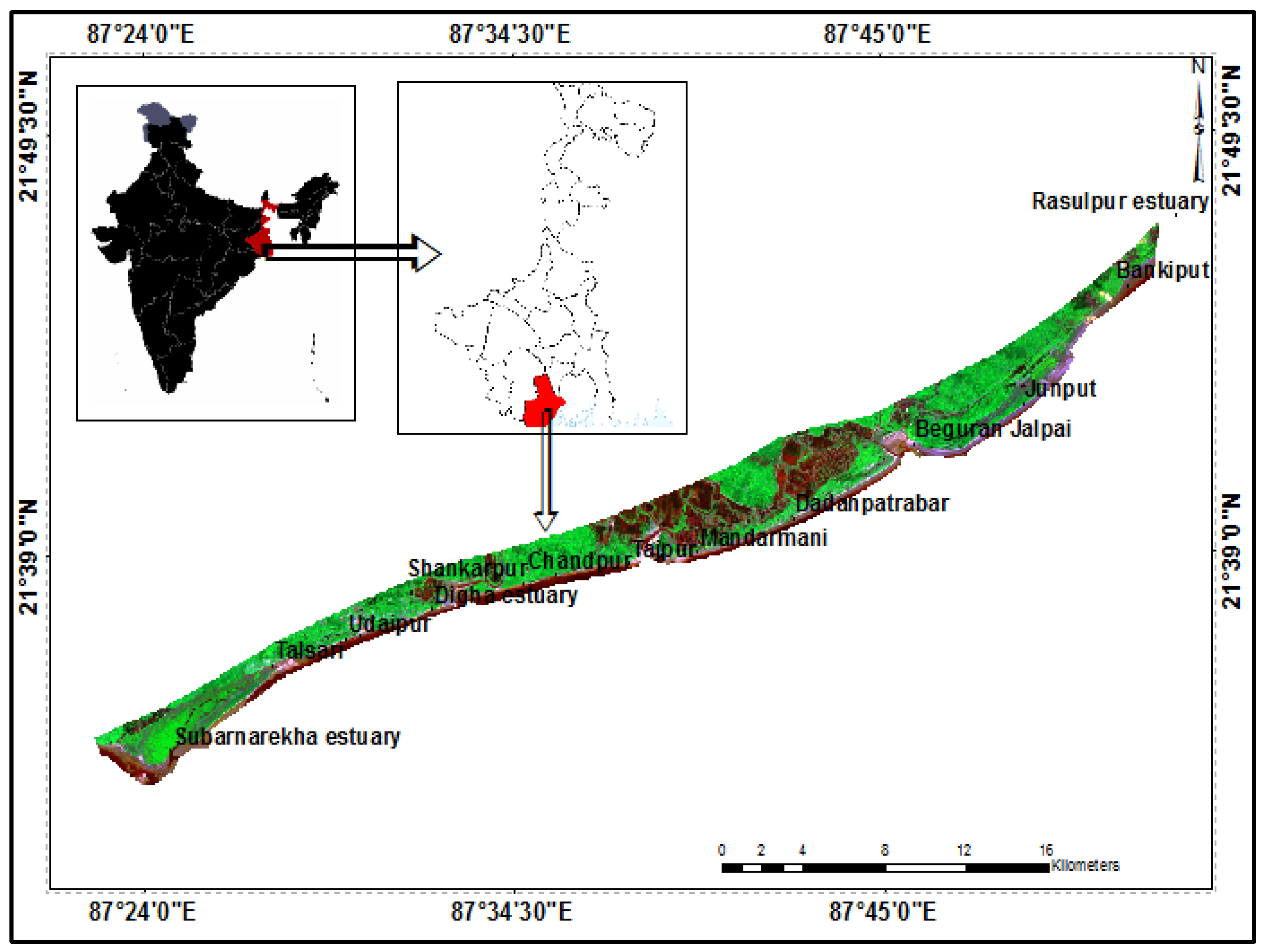
2. Study Area

This study was conducted between the areas of the Rasulpur River to the Subarnarekha River estuaries on the East Coast of India, along Purba Medinipur and the Subarnarekha delta plain connected over the states of West Bengal and Orissa, respectively (Figure 1). Using remote sensing and GIS techniques, the land-use and land-cover (LULC) changes of the coastal area were classified within a total area of 144.26 sq. km (length of coastal stretch: 70 km). The area is situated within 87°22′36″ E to 87°52′55″ E in longitude and 21°34′25″ N to 21°47′16″ N in latitude. Less than 3 m above sea level is the average elevation [61]. Quartz is the main beach sand material, and the sand is yellowish brown in color—very similar to the Subarnarekha estuary sand. This similarity indicated that the beach sand was sourced mainly from the Subarnarekha River of the study area, not from the Ganga [1]. Tropical climatic conditions have been observed over the region. An average monthly temperature of 22 °C to 34 °C was observed over the study area. The entire area is influenced by the southwest monsoon. Maximum monthly rainfall of 280 mm was observed in the monsoon season (June and July), and the lowest monthly rainfall of 1 mm was observed in the month of December [1]. The East Coast of India along the Bay of Bengal is more active with respect to inundation and ocean-associated shocks compared to the West Coast [62,63]. Regarding land utilization, the study area has experienced an increase in rapid urbanization, especially as a result of tourism activities; other economic activities (hotelkeeping, business, shopkeeping and the travel industry) are also found in the hinterland of this region, which has featured in previous research studies [1,59,64], and this urbanization has induced several risks of hazard in the study area [65,66].

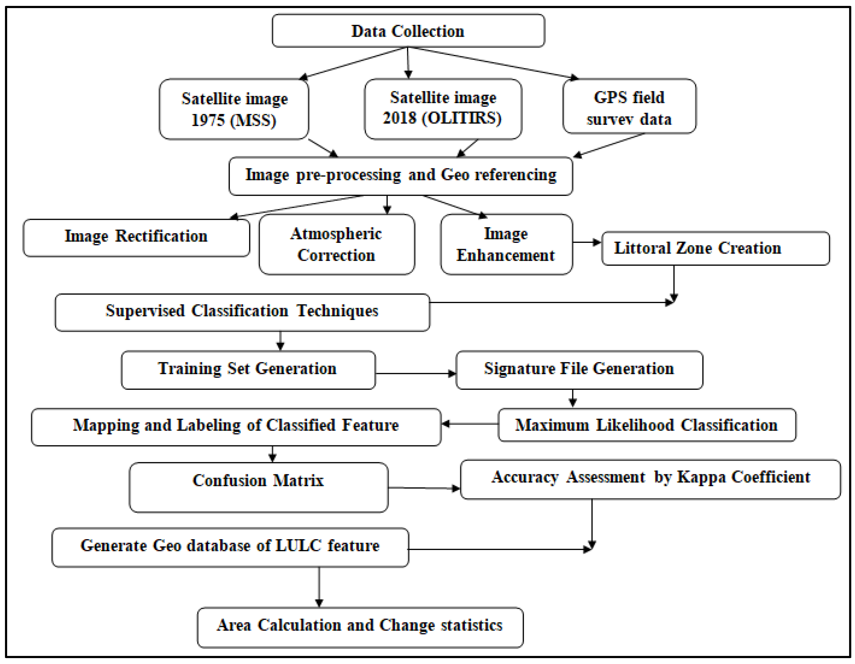
3. Methodology

3.1. Data Selection and Data Processing Techniques

Satellite images are the most significant data for the extraction of LULC information based on remote sensing techniques [67,68,69,70,71,72]. Satellite images and ground-truth data were used to classify LULC features [73].

Table 1. Details of the data used in the present study.

Year	Sensor	Resolution	Path/Row	Month	Source
1975	MSS	60 m	149/045	May	USGS
2018	OLI/TIRS	30 m	139/45	October	USGS

describes the detailed data used in LULC mapping. The data are available at https://earthexplorer.usgs.gov/ (assessed on 21 January 2020).

Figure 2 shows a schematic flow diagram of the methodology used in the study. The present study used two satellite images: an MSS image from 1975 and an OLI/TIRIS image from 2018. The MSS image from 1975 was chosen for the analysis of LULC because at that time improvised satellite images were not available, such as Landsat 7, ETM+ and Landsat 8 series images. In 2018, OLI/TIRIS series images could be applied in analysis due to the availability of high-resolution satellite images which provide the maximum accuracy for ground-truth analysis. The satellite data collected from different times (1975 and 2018) had differences in resolution. Afterward, the available images were interpreted visually for mapping, but the differences in resolution had an influence on the image accuracy with respect to reaching the real ground information for LULC mapping. The 1975 image contained some atmospheric errors due to the low relation capacity, which created obstacles in acquiring the features. This low resolution was especially observed in built-up areas in the 1975 image. However, with the help of the ground verification system through the Google Earth Historical View option, real-time feature information and a topographical map was collected and verified by the accuracy method. Landsat 8 and MSS data, by contrast, are highly reliable for coastal studies over past decades [74,75]. A period of forty-three years was chosen for the analysis, using two images (from 1975 and 2018), because the study aimed to show the long-term changes in the area. If the study had chosen 5 or 10 years as the window of analysis of LULC, then long-term changes could not have been assessed via the analysis. LULC change is a very long-term process, so the study chose 43 years as the time scale to determine the exact changes that had taken place. The selected satellite data were processed by the remote sensing and GIS application. The remote sensing data contained some geometric and radiometric flaws or errors. Due to these errors, in the first phase of processing, radiometric correction and geometric rectification methods were performed using ERDAS Imagine 2014 software. The rectified images were then exported to ArcGIS software to subset the images based on their areas of interest (AOIs). The images for 1975 and 2018 were co-registered in the projection method. The Universal Transverse Mercator (UTM) projection system with zone 45 and the WGS 84 datum was used for all the selected images. The image for 2018 was rectified by the collection of ground control points (GCPs) from the field survey through GPS. This rectification method is mainly used for enhancing and improving the quality of images. It enables reduction in atmospheric errors that cause reduced brightness in actual images, which affects digital remote sensing processes. The radiometric correction helps to minimize these errors and improve brightness quality, thus providing more accurate information about a particular area or region captured in an image. Radiometric correction can be applied to various sources, such as satellite data, aerial photography and even scanned maps, that are affected by atmospheric conditions, such as absorption, scattering due to cloudy weather, sensor calibration issues, etc. By performing this method on any such source, it becomes possible to retrieve correct values without being influenced by any external factors, such as atmosphere changes, etc. Furthermore, it also helps to increase accuracy while performing further analysis of sources, making sure that all results generated are reliable and precise, as well as free from biases due to external environmental factors. In the image from 1975, some atmospheric errors were found which reduced the brightness in the actual image. By means of the abovementioned correction, the errors were minimized and the image brightness quality was improved for the digital remote sensing process. Atmospheric absorption, cloudy weather conditions, scattering, sensor calibration, etc., may create radiometric errors in satellite data. The 1975 image rectification and georeferencing process was an important step in creating accurate digital maps. This process involved using Google Earth images to match the coordinates of a given location with the corresponding points on a map. The topographical map for 1975 was collected from the Survey of India (SOI), West Bengal, India, and was also used as a reference map for the 1975 satellite image [1]. The goal was to create an accurate representation of what that area looked like in 1975 which could be used for various purposes, such as historical research or environmental monitoring. By comparing these data with current satellite images, one can assess how much change has occurred over time and determine whether any areas have been significantly altered. Overall, though, despite some limitations, due mainly to being limited by resolution size (which affects the ability to detect small objects), rectifying/georeferencing past images using Google Earth provides us with valuable insights into our changing environment which would otherwise not be available without significant effort and resources being dedicated towards obtaining old photos manually. The use of satellite imagery for land-use/land-cover mapping is a well-established practice, and the Multispectral Scanner (MSS) has been used in numerous studies to map various types of land cover. Before using the MSS image from 1975, several literature surveys were conducted to assess its accuracy. It was found that many previous research projects had used MSS images in a global context with varying levels of success [76,77,78,79]. The accuracy assessment proved to be complex due to factors such as cloud cover and resolution limitations, but it provided valuable insight into how best to utilize this type of data for future projects. We have noted that accuracy assessment is a complex task because we wish to inform future researchers about the problems associated with using MSS satellite images. Given this information, other researchers may also be able to employ the proper methodologies to obtain the maximum level of accuracy. We also obtained information from the abovementioned literature.

3.2. Classification Method

To prepare an LULC map from satellite images, the classification is the most significant method. There are three main methods that are useful for digital image classification systems: supervised, unsupervised and hybrid classification systems. Both supervised and unsupervised classifications are involved in the hybrid classification method. Each image (from 1975 and 2018) was classified for land-cover classes separately. ArcGIS 10.3 software was used in the classification methods. The present study chose five specific features (built-up, soil, sand, vegetation and shallow-water areas) which are related to shoreline change studies and create immense pressures in terms of shoreline modification. The study area is mainly formed of sand and soil transported by the river estuaries. As the study area contains several estuaries (the Subarnarekha, Talsari, Digha, Mandarmani, Beguran Jalpai and Rasulpur estuaries), we tried to show the changes in soil, sand, vegetation, shallow-water and built-up areas. These agents are properly associated with coastal erosion, which has already been discussed in several papers concerning the study area [65]. The current study focused on five distinct characteristics that are related to shoreline change research and have enormous effects in terms of shoreline modification: built-up areas, soil, sand, vegetation, and shallow water. The selected features’ characteristics are described below:

Soil: Soil areas are a distinct landform class associated with tidal flats of coasts and estuaries, as well as waterlogged areas of alluvial plains and dune slacks. This LULC (land-use/land-cover) class is different from the more commonly known ‘mudflats’ which are mainly found in coastal regions. Muddy areas can be formed by several processes, such as sediment transport, erosion, deposition and human activities, including construction and agriculture practices that lead to changes in the landscape.

Sand: Beaches, frontal dunes and bare interior dunes are all areas that have sand as the dominant feature.

Shallow water: Depressions that mainly contain stagnant water with low suspended sediments can be found in many different forms. Palaeochannels are ancient riverbeds which have been filled with sediment over time and now contain standing water.

Vegetation: The vegetation found within reserved forests is incredibly varied depending on where you look in them; however, there are certain species that will always be present regardless of location or habitat type, such as mangroves, which require specific conditions to survive but which, once established, can become dominant features throughout entire reserves, with only small pockets being dominated by other plant types, such as salt marsh grasses or sea grasses—all three playing vital roles in maintaining healthy coastal environments.

Built-up areas: Any kind of manmade structure, such as hotels, motels, parks, industrial units, houses and shops, can be found within built-up areas.

The selected features were chosen due to their direct association with coastal erosion processes and erosional activities along shorelines. Mangrove vegetation has also been planted near shoreline areas for protection against coastal erosion, acting as a soft-protection mitigation strategy for beaches. Naturally occurring mangroves are found predominantly in the Sundarban region of West Bengal, India—an area that experiences high levels of tidal activity from the Bay of Bengal, making it particularly vulnerable to coastal erosion processes, such as wave action and sediment movement due to currents or tides, leading to beach loss or landward retreat over time if not properly managed through protective measures, such as mangrove planting initiatives, which have been taken by the local authorities there. Salt production on the East Coast of India is rare, with most of the production concentrated on the West Coast. The study does not focus on salt production because the aim was to determine the land-use/land-cover pattern changes related to coastal erosion. Shrimp cultivation has been observed to take place mainly in sheltered areas, such as inland bays and estuaries.

To interpret the LULC changes properly, the study area was divided into three littoral zones. Littoral zones are areas along the shoreline of a body of water. These areas can be divided into three distinct types: estuaries, deltas and beaches. Estuaries are bodies of water where rivers meet the sea and they contain brackish water with high levels of nutrients, making them ideal habitats for many species. Deltas form when sediment is deposited by rivers in shallow coastal waters, creating unique environments that support different forms of aquatic life to other regions nearby. Beaches occur on coasts where waves break against landforms, such as cliffs and sandbanks, creating areas rich in biodiversity due to the constantly changing nature of wave action, tides and storms. In order to study these littoral zones more effectively, it is important to select specific locations based on field surveys which take into account both physical characteristics, such as sedimentation rate, and conditions of material supply, such as nutrient availability, depending upon the region studied. In this case, we selected three littoral zones based on their locations relative to estuaries found within our study area. The area of LZ I sediment was supplied by the Subarnarekha River, while LZ II sediment was supplied by the River Ganga and LZ III sediment was sourced from the Ganga and Rasulpur River estuaries. The littoral zones are:

• Littoral Zone I: The Subarnarekha estuary to Digha estuary coastal stretch, along with Talsari, Udaipur, Old Digha and New Digha (total area: 38 km²);
• Littoral Zone II: The Digha estuary to Beguran Jalpai coastal stretch, along with Chandpur, Tajpur, the Mandarmani estuary, Mandarmani and Dadanpatrabar (total area: 70.05 km²);
• Littoral Zone III: The Beguran Jalpai to Rasulpur coastal stretch, along with Junput and Bankiput (total area: 36.21 km²).

After generating the littoral zones, the training samples were created for image classification. Training sample collection is a more accurate method for comparisons with raw samples of field data. After performing the training modules for each feature, the training file was generated for the further classification process. In selecting an accurate training polygon for each class, the uniformity of the polygons was the most significant property, and their representation was significant throughout the images for each class [80].

The supervised classification system was carried out by applying training areas. Finally, the accuracy assessment was performed for each classified map. An appropriate change detection map can be obtained from accurately classified images [54]. Sand, soil, shallow-water, vegetation and built-up areas were selected as feature classes to show the changes near the shoreline area in the selected time period (1975–2018).

Algorithm: A maximum-likelihood algorithm was applied to identify the land-cover pattern using ArcGIS 10.3 software. This algorithm was applied in the classification stage. This algorithm is associated with the signature of a particular training sample depending on the probability density process. Based on the probable priority, pixels are imposed with respect to each signature [50,52,54,81]. A significant proportion of the least-probable pixels can be eliminated from the classification. This type of algorithm is also termed a Bayesian classifier because these algorithms have the ability to incorporate knowledge using Bayes’ theorem [82]. A priority of probability could be expressed by the knowledge which exists regarding each feature class. This can be justified as an individual value that is appropriate for all pixels.

3.3. Accuracy Assessment

Accuracy analysis is the final step of the classification method. It is a statistical process which evaluates the classified image. An integrated process of LULC feature extraction is accuracy assessment from classified images. From this assessment, errors are marked in the classified image and improve the quality of the derived information [83]. Without assessing the accuracy, no image classification can be considered accurate [84]. To assess the accuracy of a classified image, a confusion matrix is the standard means of measurement [17,85,86,87,88]. With such a matrix, pixels are gathered according to their similarity or dissimilarity by comparing a ground-truth pixel with a location in the classified image. In the kind of confusion matrix used here, reference data are represented by columns and pixels in a class depicted by rows in a classified image [89]. With the help of three kinds of measurements, the confusion matrix was completed: user’s accuracy, producer’s accuracy and overall accuracy assessment depending on the omission and commission error rates [90,91,92]. In a classified image, random points were chosen with two sets of class values for the utility list. This accuracy analysis was applied for the 1975 and 2018 LULC maps. In the present study, this accuracy analysis was a more complicated task for the 1975 LULC map because of the lack of available reference ground-truth data and low-resolution satellite data. Google Earth high-resolution images were also used as reference images for the accuracy analysis. The Google Earth ‘Historical View’ mode is an invaluable tool for researchers studying changes in landscapes over time. By using this feature, researchers can identify the position of a given feature as it appeared in a certain year, such as 1975, and compare it with current images from Google Earth. This allows them to track changes that have taken place since then, providing valuable insight into how land use has changed over time. In addition to using Google Earth’s Historical View mode, other high-resolution images of past years may also be used for research purposes. For example, recent research aimed at showing long-term changes between 1975 and 2018 was carried out with the help of MSS 60 m resolution imagery, which provides much more detail than is available in Google Earth alone. By combining both sources together, researchers are able to obtain a comprehensive view of how land use has evolved over decades or even centuries. The ability to accurately track large-scale environmental change through time helps us better understand our planet’s history in a way that would not be possible without these technological advancements. Accuracy assessment using the Google Earth system is a crucial part of any data analysis. It ensures that the information being collected and analyzed is accurate and reliable. The topographic map reference data from 1975 provided an important resource when evaluating current datasets obtained through modern technologies, such as Google Earth. By comparing new findings against older reference materials, researchers can more accurately assess how much change has taken place over time; this helps to ensure that any conclusions drawn based upon these analyses will be valid, even if conditions have changed since the earlier time.

The accuracy assessment was also part of developing the confusion matrix for maximum-likelihood classification. This kind of matrix shows omissions (producer’s accuracy) and commissions (user’s accuracy) and, finally, Kappa coefficient statistics for classified images.

The sum of correctly classified pixels divided by the summation of all pixels provides the overall classification accuracy for a classified image. The reliability of the user’s accuracy with respect to commission errors describes the probability that a pixel that is classified on a map truly represents the land-cover type on the ground [93]. Omission errors correspond to the producer’s accuracy. For the overall accuracy analysis, the diagonal elements were used in the confusion matrix.

Samples were randomly selected in the LULC map. Every sample point was verified with Google Earth high-resolution images. Each corrected sample counted as 1 if it was matched with the ground-truth point in Google Earth, and the incorrect matches were counted as 0. Finally, the error matrix was stored from the summarization of all the collected information. This method is the one that has been most frequently used by recent researchers for accuracy analysis [87]. Overall accuracy is represented by the following equation:

$$\frac{\sum _{a-1}^U{C}_a}{Q}\ast 100$$

(1)

where Q and U are the total numbers of pixels and classes, respectively. The minimum value which is acceptable for overall accuracy is 85% [94,95,96].

The Kappa coefficient method is a distinct multivariate application formed by Cohen [97]. This method was applied for LULC accuracy assessment in the classification system. In this error matrix, pixels are computed for coefficient values depending on the difference between the total row and column chance agreement and the actual agreement of the error matrix [90,97,98,99]. Kappa values are demarcated as follows:

$$K=\frac{\sum _{a-1}^U\frac{C_a}{Q}\sum _{a-1}^U\frac{C_{a{C}_{a·}}}{Q^2}}{1-\sum _{a-1}^U\frac{C_{a·C_{a·}}}{Q^2}}$$

(2)

where C_a = the row sum.

4. Results and Discussion

4.1. Spatial and Temporal Changes in LULC between 1975 and 2018

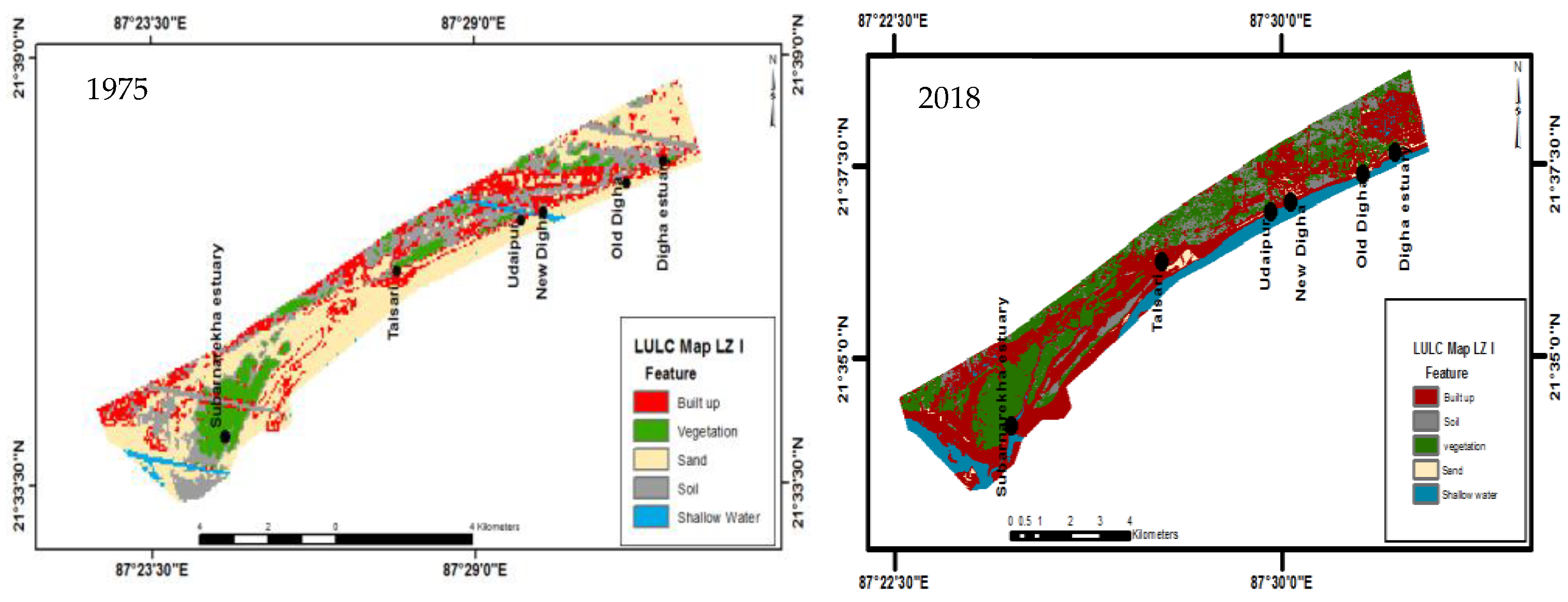
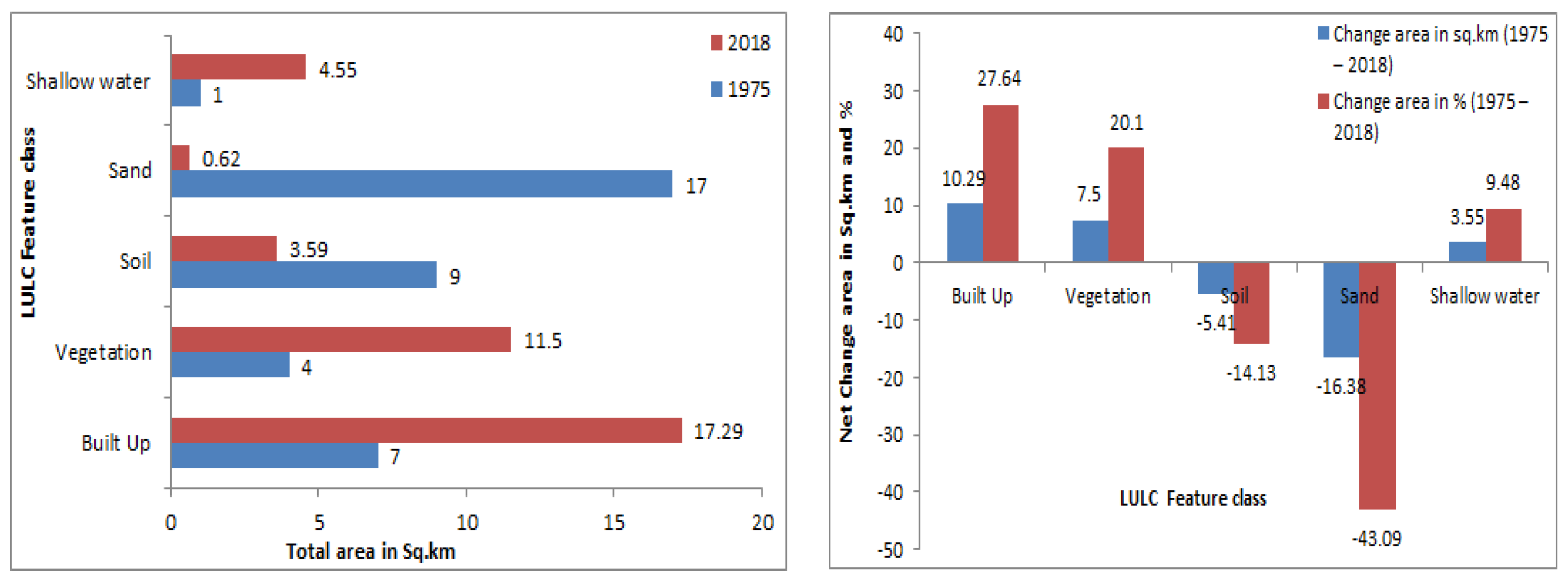
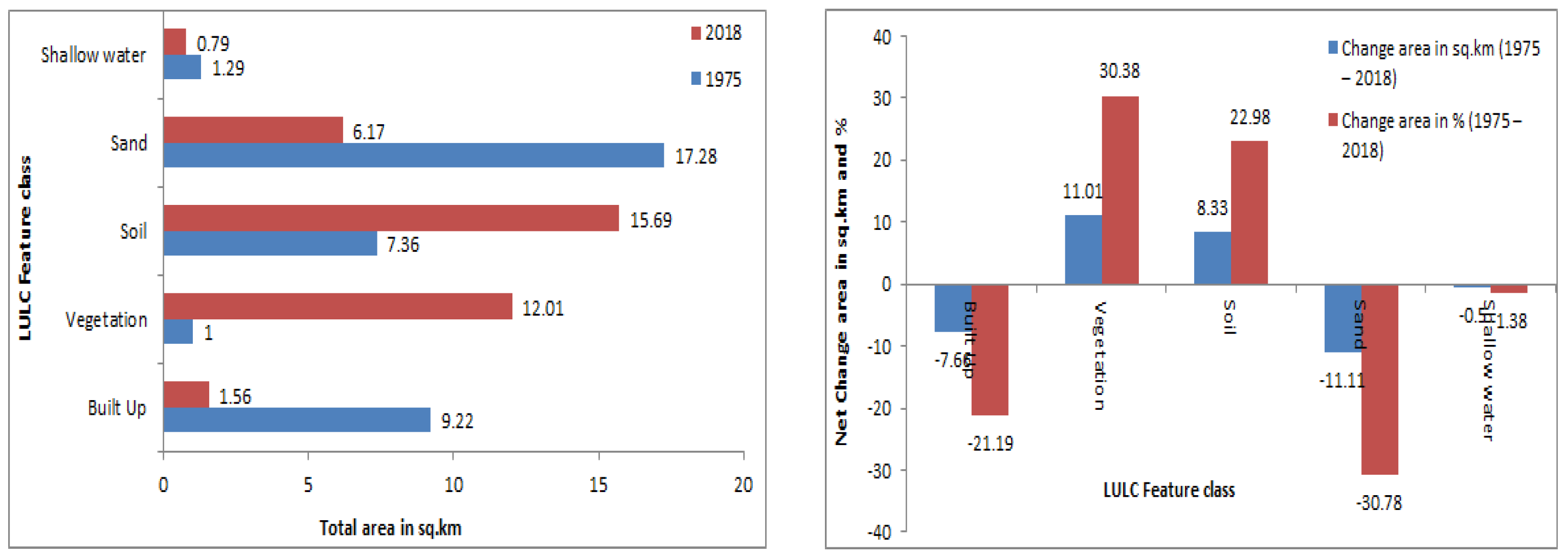
4.1.1. Land-Use/Land-Cover Assessment of Littoral Zone I

Sand was a dominant feature in 1975 and was occupied by built-up areas in 2018 (Figure 3). Dense vegetation was identified near the estuary area in 1975, but in 2018 the area of vegetation increased in a spatial way (Figure 3). The maximum soil area was noticed in the year 1975 (Figure 3) and was occupied by built-up areas in 2018 (Figure 3). Shallow-water areas were not visible in 1975 but were observed to have increased in 2018, a prominent rapid expansion being found in the year 2018 (Figure 3). This trend of increase indicates prominent shoreline shifting or changes in the study area.

Talsari, New Digha and Old Digha showed evidence of rapid expansion of built-up areas. The maps for 1975 and 2018 (Figure 3) revealed that important land-use and land-cover changes had occurred throughout LZ I. In the map for 1975, the intensity of built-up areas was observed inland (Figure 3), providing evidence of the domination of soil in the entire area and that the built-up areas had shifted nearer to the shore in a very few areas. Sand was almost absent from the Old Digha area and found only in the Talsari and Udaipur beach areas. However, a dominative increase in shallow water was observed from Talsari to the Old Digha area. By contrast, the other image, from 2018 (Figure 3), depicted the increase in urbanization in the Old Digha, New Digha, Talsari and Digha estuary areas. Shallow water was observed to have rapidly increased by the year 2018. However, vegetation areas reached a maximum in 2018 (Figure 3). The vegetation area also expanded due to the initiative of the River Research Institute (RRI) to protect the coastal zone, mangrove plantation being considered a soft protection strategy (reported by the RRI field survey in 2019). With close examination of Figure 3, one can observe a rapid expansion of urban areas over time.

Within the 43-year (1975–2018) span, the change analysis showed that the 7 km² built-up area which can be seen in Figure 4 increased to 17.29 km², whereas the soil area reduced to 5.42 sq. km during this period. The vegetation area increased from 4 km² to 11.5 km² in the 1975 to 2018 time period. A prominent increase was noticed in the shallow-water area from 1 km² to 4.55 km². The present research task was a land-use and land-cover analysis, and thus did not consider shoreline movement. Shallow-water area (loss and gain) was estimated in this research. The land loss observed was due to the loss of sand area, the 17 km² sand area having reduced to 0.1 km². The total sand area was reduced by 16.38 km².

4.1.2. Land-Use/Land-Cover Assessment of Littoral Zone II

Shankarpur, a muddy area, was laid over the zone in 1975, and the urban area was observed as the dominant feature. A limited area was occupied by vegetation in 1975 (Figure 5), but the vegetation area was expanded in 2018. In the map for 2018 (Figure 5), the soil area shifted to vegetation in the Shankarpur coastal area. In 1975, the sandy area was seen from Shankarpur towards the Digha estuary area, but in 2018 the entire sandy zone was absent and was scattered near the shoreline zone, where a prominent shallow-water increase was identified (Figure 5).

Chandpur and Tajpur, two coastal areas, were dominated by sandy areas and built-up areas in 1975 (Figure 5). A close look at the 2018 map revealed the expansion of the vegetation areas in the Chandpur to Tajpur area (Figure 5). Very few areas were observed as shallow water in the 1975 classified image, but from 2018 a remarkable enhancement was noted over the coastal stretch.

The Mandarmani estuary, Mandarmani and Dadanpatrabar are very important regarding the expansion of built-up areas very near to the shoreline. In 1975, the built-up areas were observed in or near shoreline areas and also spread to inland areas (Figure 5). However, in 2018, the built-up areas had shifted near to the shoreline, where shallow-water influence was also observed. The domination of the vegetation area was only marked in 2018 over the region. A muddy area was identified in 1975, but it was occupied by built-up areas in the 2018 map. The sandy area was observed to have undergone negative growth over the time period; only the 1975 map showed an intense increase in sandy areas over the region.

The Dadanpatrabar to Beguran Jalpai area was mostly expanded by built-up areas over the period (1975–2018). Muddy and sandy areas were found in the 1975 map, and a small zone of sand was noticed in the map for 2018. The vegetation area was dominated by other features in the 2018 map.

Figure 6 shows that built-up areas had reduced in 2018 from 1975, with a reduction of 8.55 km². A prominent temporal change was noticed in the vegetation area, which increased from 2.82 km² to 15.46 km², which means that there was 12.64 km² of growth in vegetation areas in the study area. Proper loss of sedimentation was found during this time period within this zone, with 12.65 km² and 5 km² of soil and sand demolished, respectively, by the increase in shallow water. The shallow-water area of 1.7 km² increased to 13.56 km², meaning an increase of 11.86 km² in shallow-water zones. This increase in shallow water indicated the shifting of the shoreline during the time period (1975–2018). In recent years, the West Bengal government in India has been taking steps to enhance shallow-water protection strategies in this region. This effort involves strengthening existing policies and introducing new ones that promote sustainable management practices. The aim is to ensure that coastal ecosystems are preserved while also providing economic benefits from fishing activities and other uses of aquatic resources (source: RRI). The report collected by the tourism department in 2018 revealed that maximum soil areas have been converted into vegetation areas. This is due to several factors, including climate change and human activities, such as urbanization and deforestation. As a result of these changes, there has been an increase in tourist activity along the littoral zone, which has led to the rapid development of hotels very close to the shoreline. According to a report by the River Research Institute (RRI), West Bengal, India (2018), the area of LZ II has seen a loss of built-up areas due to enhancement of the vegetation near the shoreline. It was also observed that the area of LZ II was used for shrimp cultivation and small fisheries near the inlet areas. An extensive field survey was conducted in the study area in 2016–2018 to find out the reason for the loss of built-up areas. The RRI data are also helpful in understanding the enhancement of soft protection strategies in this particular zone to protect the shoreline from coastal erosion. After completing the LULC map, the obtained data were also verified with the official data of the RRI.

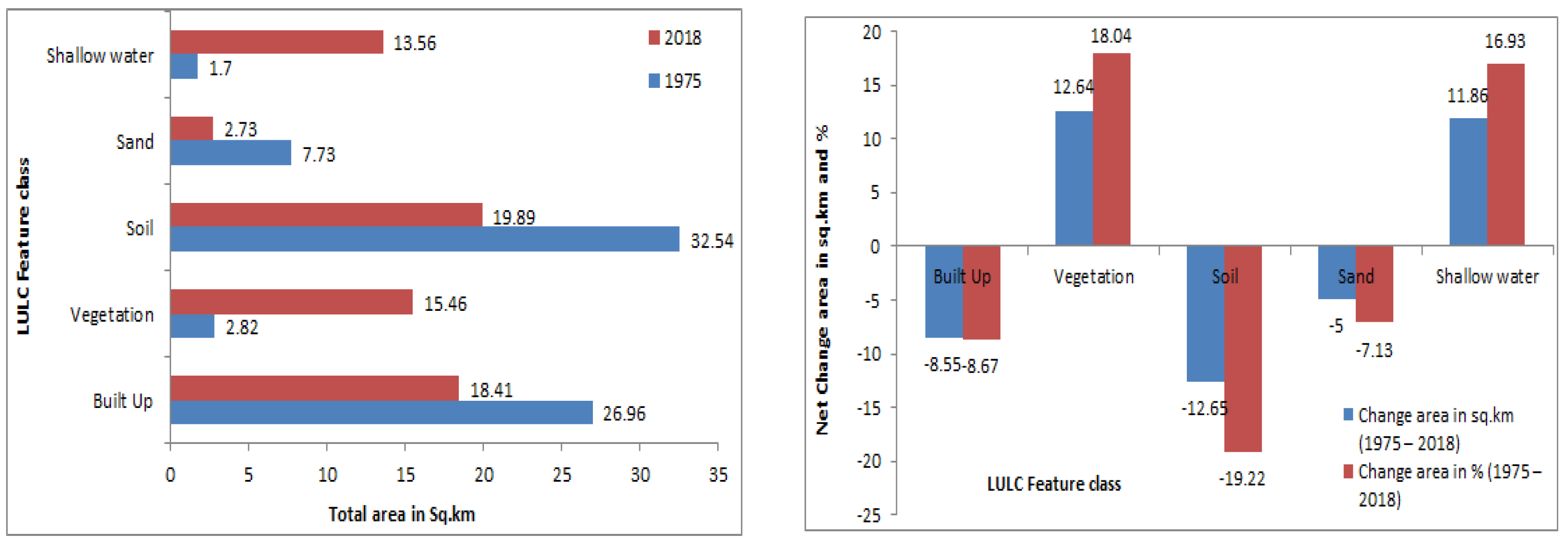
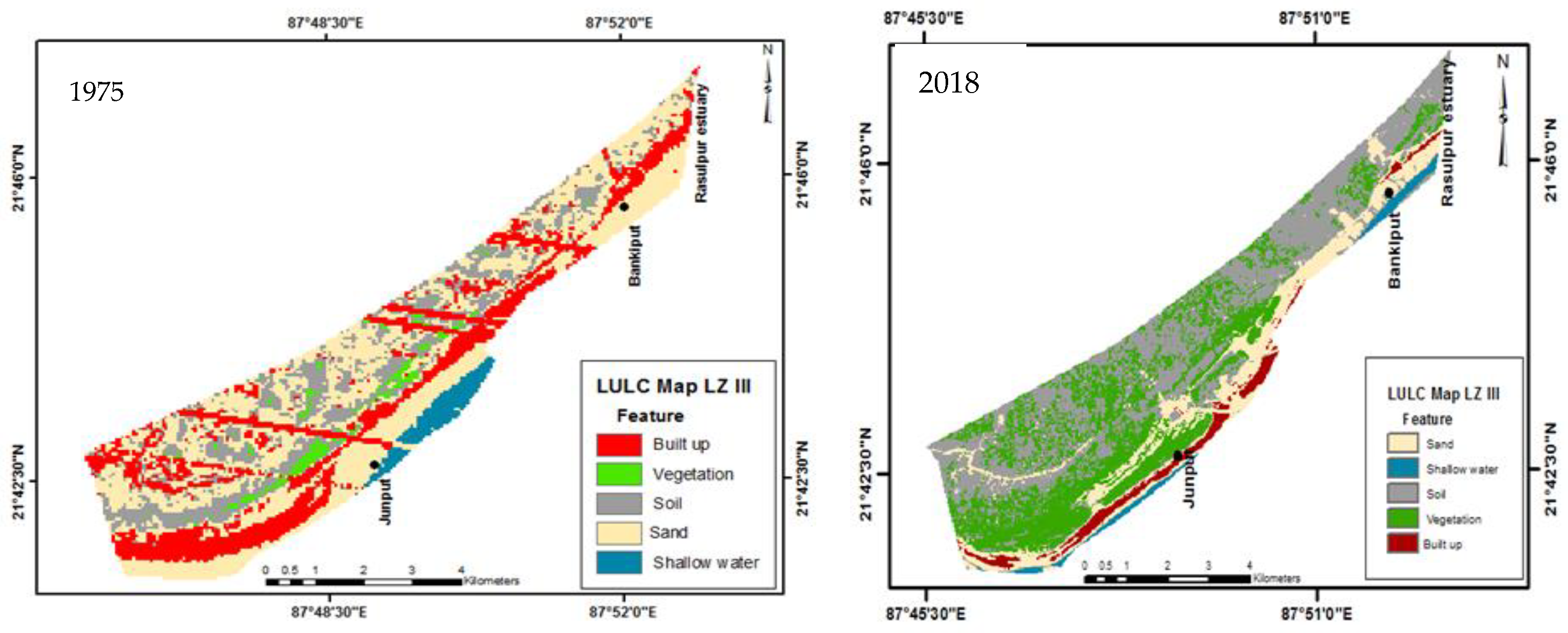
4.1.3. Land-Use/Land-Cover Assessment of Littoral Zone III

Figure 7 shows the change dynamics in Junput, where, in 1975, most of the area was covered with sand, while in 2018 the muddy areas had become sandy areas. This muddy area expansion was due to the enhancement of built-up areas. In 2018, the muddy area was transformed into a vegetation area. Redundancy of vegetation was also observed in 1975. A very remarkable observation in this zone was that the existence of shallow water was much reduced in the Junput area. Only in 1975 was a prominent shallow-water level observed over the four decades. In 2018, a small area contained shallow water along the Junput coastal stretch.

The Bankiput coastal area in the year 1975 exhibited a concentration of sandy areas which was eliminated by soil in 2018. The image for 2018 (Figure 7) shows that shallow-water levels had encroached into sandy areas and that built-up areas were also decreased.

The Rasulpur estuary is one of the important estuaries in Purba Medinipur District (West Bengal). Sand deposition was evident in 1975 (Figure 7), and a small built-up zone was also found near the estuary. The vegetation in 1975 was eliminated over the area. The muddy area was also found to be in a poor condition. In the 2018 image, the advancement of shallow water with the deposition of sand and soil near the estuary area could be observed.

From Figure 8, it was noticed that maximum increases were found in the vegetation and soil areas. A 1 km² area of vegetation in 1975 grew to 12.01 km² in 2018. Regarding soil area, 7.36 km² in 1975 increased to 15.69 km² in 2018. However, this littoral zone showed negative changes in built-up and shallow-water areas, with 7.66 km² lost from built-up areas and 0.5 km² lost from shallow-water areas. A few areas in LZ III have not developed as have the other parts of the study area (LZ I and LZ II). For this reason, the LZ III population shifted towards LZ I and LZ II, and tourism is also very limited in this particular zone. By contrast, the Bankiput coastal zone was found to be subject to coastal erosion [100]. Seawall protection strategies have been also observed in the Bankiput region, with a combination of soft protection techniques employed.

4.1.4. Comparison of Differences in Land Use/Land Cover in the Three Littoral Zones

The LULC classes were derived from multi-resolution satellite images for five land-use/land-cover classes—soil, sand, vegetation, built-up and shallow-water areas—covering a period of 43 years from 1975 to 2018. The changes in the land use/land cover were also identified. The land-use change analysis has been presented on a spatio-temporal scale. The observed important changes are summarized below.

The present study of land use and land cover in LZ I over the past 43 years (1975–2018) revealed some interesting trends. Firstly, there has been a significant increase in built-up areas from 18.42% to 46.06%. This demonstrates increased urbanization within the region, which is likely due to population growth or other economic factors that are driving people towards this particular location. Secondly, vegetation areas have experienced limited growth, from 10.53% to 30.63%, with maximum growth being observed in 2018, indicating that efforts are being made by local authorities or individuals at conservation within this area of LZ I. Thirdly, soil areas have fluctuated significantly over the 43-year period, with values ranging between 23.68 and 70.68%. However, during 2010–2018 soil areas reduced considerably, suggesting that degradation may be occurring as a result of human activities, such as farming practices, deforestation, etc. Sandy areas also showed similar signs, with the original area of 44.74% being reduced to 1.65% in 2018, possibly due to shallow-water enhancement taking place as a result of irrigation methods and other non-natural causes, such as construction activities. Lastly, the shallow-water area was found to have increased linearly throughout the period, from 2.63% (1 sq.km) to its peak at 17.75% (4. 55 sq.km) in 2010 before settling back down to slightly lower than the initial levels.

In LZ II, it was observed that the built-up areas were not much extended compared to LZ I. The study has depicted the trend of decrease in built-up areas, from 26.96% (34.95 sq.km) to 18.41% (26.28 sq.km) within 43 years (1975–2018). The vegetation area increased over this time period, from 2.82% (4.13 km²) to 15.46% (22.07 km²), and soil area decreased from 32.54% (47.61 km²) to 19.89% (28.39 km²). Fluctuations in muddy areas were also observed in the study region (LZ II); a sudden increase in soil cover of 36.62% (52.28 km²) was noticed in 2010. A negative trend for sand over the time period was observed, with a 7.73% (11.03 km²) area of sand in 1975 being eroded to 2.73% (3.90 km²) in 2018. The change analysis marked a sharp expansion in the shallow-water area, which extended from 1.70% (2.49 km²) in 1975 to 13.56% (19.36 km²) in 2018. In this entire littoral zone, only shallow-water areas showed proper expansion, with prominent positive growth lines from 1975 to 2018.

LZ III showed a negative trend for built-up areas over the 43 years, these being reduced from 9.22% (25.49 km²) to just 1.56% (4.30 km²). A negative trend was also experienced for sand areas, which decreased from 17.28% (47.80 km²) in 1975 to 6.17% (17.02 km²) in 2018. Positive growth trends were observed in vegetation and soil areas within the 43-year period. The initial vegetation area of 1.00% (2.78 km²) in 1975 increased to 12.01% (33.16 km²) in 2018, and the initial soil area of 7.36% (20.35 km²) extended to 15.69% (43.33 km²), which is a remarkable extension over the time period. It is very significant that no major change was observed in shallow-water level over the period; only some short-term changes in shallow water occurred between three time periods (1975–2000, 2000–2010 and 2010–2018). The 43-year analysis of shallow water showed stagnation, with an area of 1.29% (3.57 km²) in 1975 and an area of 0.79% (2.19 km²) in 2018.

This change analysis shows that most of the changes occurred due to manmade activities as a result of human encroachment and the expansion of tourism industries and urban transformation over the entire area. The transgression of the shoreline is the major problem observed in the present study.

4.2. Accuracy Assessment

The accuracy assessment was performed to check the authenticity of the classes examined using the four maps (1975 and 2018). From this assessment, it was determined whether the features were underestimated or overestimated. A confusion matrix was prepared for each map for 1975 (total area: 144.26 km²) and 2018 (total area: 144.26 km²).

Table 2. Confusion matrix of LULC maps for 1975 and 2018.

LULC Feature Name	Producer’s Accuracy		User’s Accuracy
	1975	2018	1975	2018
Built-up	100%	71.43%	57%	71.43%
Vegetation	70%	100%	87.50%	100%
Soil	87.50%	71.43%	100%	100%
Sand	84.1%	100%	77.77%	90%
Shallow water	100%	100%	100%	89%
Overall accuracy			85%	90%
Kappa co-efficient			80.83%	87.43%

shows the confusion matrix for the 1975 and 2018 data, for which an 85% overall classification accuracy and a Kappa statistic of 80.83% were obtained. The maximum accuracy was found for the built-up areas and shallow-water areas with respect to producer’s accuracy, but with respect to user’s accuracy, vegetation and shallow water showed the highest accuracy for 1975. The maximum producer’s accuracy was obtained for built-up, soil and shallow-water areas, and the highest user’s accuracy was acquired for vegetation, sand and shallow-water areas. A 90% overall classification accuracy and an 87.43% Kappa accuracy were obtained for the 2018 map. In the case of producer’s accuracy, vegetation, sand and shallow water were identified as having the highest accuracy levels. Vegetation and soil with respect to user’s accuracy reached the highest accuracy value (100%). Sand and shallow-water accuracy showed remarkable accuracy values of 90% and 89%, respectively. In some cases, the user’s accuracy and producer’s accuracy were misclassified due to image-resolution problems for the image from 1975. However, overall, these error matrices showed good similarity between the classified features and the ground features. The accuracy assessment not only employed the Google Earth system, a topographical map from 1975 was also used as a source of referential data for the accuracy measures. In addition to using Google Earth, a topographical map of 1975 was also used for accuracy measures. Topographical maps are especially useful when assessing data from before digital mapping systems became available or for areas where digital mapping may not be as precise as needed. Topographical maps are ideal for measuring long-term trends or identifying specific differences between different points in history, such as 1975 versus present-day conditions. A strip was also found under built-up areas during the analysis. After the accuracy assessment, it was observed that a few pixels were misplaced, but these were few in number, and this misplaced accuracy was shown in the user’s accuracy (57%). Due to this, the topographical map was used to assess accuracy.

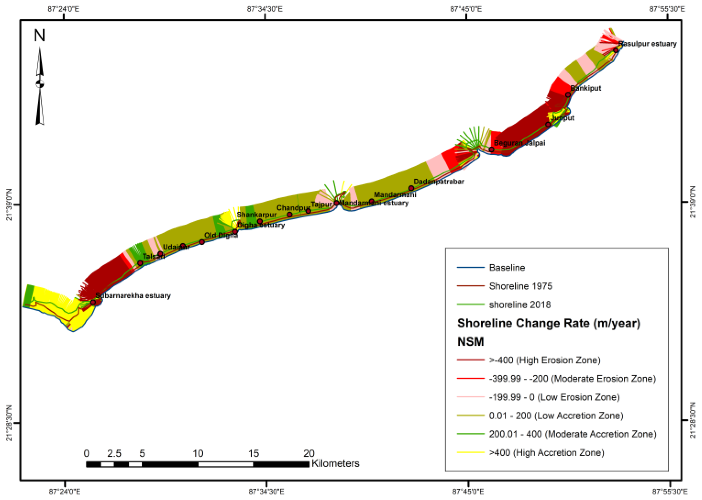
5. Erosion/Accretion Rates in the Three Littoral Zones

After analyzing the land-use/land-cover change over the period of 1975 to 2018, the study focused on the change in the rate of shoreline erosion and tried to identify the erosion/accretion zones in the study area. The shoreline is a critical component of any coastal environment, and its accurate extraction from satellite images can be an invaluable tool for environmental monitoring. Extracting the shoreline from a single-band satellite image requires careful consideration of the reflection properties of ocean water in infrared bands. When compared to land features, which have higher values than zero in infrared bands, ocean water has a value close to zero in these same bands. As such, histogram threshold methods must be applied when extracting the shoreline so as not to confuse it with other land features that may appear similar in satellite imagery due to their similar reflectance characteristics. When extracting a coastline from a single-band image using this method, band 5—mid-infrared—is often chosen, as it provides more reliable results than other available options due its superior resolution and contrast capabilities relative to other wavelengths within the visible light spectrum (i.e., red or green). This allows users greater accuracy when distinguishing between land features and bodies of water in remote sensing imagery [100]. Mid-infrared (band 5) is an important tool for distinguishing between water and vegetation/land. This band has a very low reflectance when it comes to water, whereas vegetation and soil have significantly higher levels of reflectance. As a result, this makes it easy to differentiate between land and water features in an image. In order to ensure accurate classification of land and water pixels, threshold values are used which allow all pixels classified as ‘water’ to be converted into one feature, while all pixels classified as ‘land’ are converted into another feature.

This process creates what is known as a binary image or image 1, where each pixel can either have the value zero (for non-water areas) or one (for areas with bodies of waters). To further refine these images, there exists another method that uses both band 4 and band 5, along with other bands, such as 2, which helps to create more detailed imagery, known as image 2. Using this method, water and land features can be sharply separated. A pixel value of one is considered a water pixel, and a value of zero is considered a land pixel. After acquiring image 2, both images 1 and 2 are multiplied. Finally, a binary image is obtained.

The erosion/accretion zonation mapping is an important tool for coastal engineering and management. It helps to determine the rate of shoreline change over time and identify areas that are particularly vulnerable to erosion or accretion. In order to complete this type of mapping, the net shoreline movement (NSM) technique can be used. This method involves calculating the distance between two consecutive shorelines in order to estimate long-term changes in a given area over time.

With this method, the distance between the youngest and oldest shorelines was estimated for each transect for 1975 and 2018. To calculate the shoreline shifting rate, the Digital Shoreline Analysis System, which is the most significant extension of Arc GIS software, was employed, using statistical techniques and the positions of multiple shorelines [101]. To calculate shoreline movement, the necessary elements are: (1) a baseline with the required attributes, (2) buffer creation and (3) the acquisition of shoreline positions with the proper attributes. For the present study, two shoreline positions (1975 and 2018) were acquired with the acquisition date, month and year. For change-rate analysis, transects are plotted perpendicular to the baseline. From the transects of shoreline intersections with the baseline, the change-rate statistics are calculated. The outcome of the calculation is expressed in m/year units along the transect. To calculate these change rates, GIS and remote sensing are the most-recognized tools and technologies, their application providing coastal information in digital format [102,103,104].

A zonation map was prepared to show the erosion/accretion zone over the study area based on NSM calculation data (Figure 9). The entire study area (LZs I, II and III) was divided into sets of three specific zones based on the obtained change rate for NSM: high erosion, moderate erosion and low erosion; and high accretion, moderate accretion and low accretion. From the analysis, it was observed that the Subarnarekha estuary fell in a high-accretion zone (28.49 m/year). Talsari (−24.34 m/year), the Mandarmani estuary (−31.48 m/year), Beguran Jalpai (−26.64 m/year) and Junput (−20.46) were observed to be high-erosion zones (

Table 3. The overall net shoreline movement (NSM) for 1975–2018 along the stretch from the Subarnarekha to the Rasulpur estuaries.

Littoral Zone (LZ)	Sl. No.	Name of the Shoreline	Net Shoreline Movement (NSM) in m/Year (1975–2018)	Remarks
LZ I	1	Subarnarekha estuary	28.49	Seawall (2018)
	2	Talsari	−24.34	No protection measures
	3	Udaipur	1.28	Seawall
	4	New Digha	1.25	Seawall (2014)
	5	Old Digha	0.92	Seawall (1995 and 1998)
	6	Digha estuary	5.49	Tetrapod groins (2007)
LZ II	7	Shankarpur	3.23	Seawall (2014)
	8	Chandpur	2.94	Seawall (2014)
	9	Tajpur	−1.08	No protection measures
	10	Mandarmani estuary	−31.48	No protection measures
	11	Mandarmani	−0.74	No protection measures
	12	Dadanpatrabar	1.07	No protection measures
	13	BeguranJalpai	−26.64	No protection measures
LZ III	14	Junput	−20.46	No protection measures
	15	Bankiput	−1.23	Seawall (2018)
	16	Rasulpur Estuary	−8.02	No protection measures

). Udaipur to Chandpur (including New Digha, Old Digha, the Digha estuary and Shankarpur) were found to be low-accretion zones (Figure 9 and Table 3). Mandarmani (0.74 m/year) and Dadanpatrabar (1.07 m/year) fell under low-erosion and low-accretion zones, respectively. The Subarnarekha estuary area was shown to have undergone the maximum changes over the time period, with high-accretion, moderate-accretion and high-erosion zones having been observed prominently. The most notable change that has occurred in this region is a gradual increase in landmass within certain areas where there was once only water or marshland. Based on the field survey, the mitigation strategies intended to address the beach conditions of the study area are noted in Table 3. These results are significant for future protection strategies to protect the most exposed beaches from coastal erosion.

6. Conclusions

The present study shows decadal changes in and transformation of LULC features. Remote sensing and GIS applications have no substitute techniques to obtain information about and for the monitoring of physical agents operating at the earth’s surface at periodic intervals. The ArcGIS 10.3 software environment was used in this study to compute and analyze the change rates for LULC. The study reflects that the entire area has been changed in a continuous process over the time period considered. Decadal transformation of LULC is a key agent or phenomenon in assessing coastal hazards and vulnerability due to physical and manmade activities. The entire sector of the chosen area was divided into three littoral zones to clearly identify the changes over the 43-year time period, and the changes are listed below:

❖

The study observed that areas of sand and soil were converted into built-up areas due to human encroachment and expansion of the tourism industry. It was observed that an initial 7 km² built-up area increased to 17.29 km² over 43 years in LZ I. This change had an immense effect on sand areas, with 17 km² of sand areas reduced to 0.1 km². Built-up area enhancement was not observed in LZ II compared with LZ I, where a 26.96 km² area decreased to 18.41 km². The decrease in sand and soil areas created immense pressures on existing coastal land, and thus coastal erosion occurred in the entire study area. The transformation was also observed in vegetation areas across the three LZ areas.

❖

The maximum vegetation area was observed in 2018 in LZ I, and it also helped to reduce the coastal erosion in this particular zone (according to a field survey and a report by the RRI of 2019). Vegetation expansion was highly noticeable in LZ I and LZ II, where there were 7.5 km² and 12.64 km² increases over the time period, respectively.

❖

Major changes were observed in shallow-water areas. An area of 1 sq.km of shallow water increased to 4.55 km² in LZ I, and a 1.7 km² water area changed to 13.56 km². This alteration involved the shoreline changes in the study area. However, only a decrease in shallow-water area was observed in LZ III, which was 1.29 km² in 1975 and 0.79 km² in 2018.

❖

The decrease in soil and sand areas in LZ I and LZ II provides evidence of erosion in the coastal zone, which is a major contribution of this study. In the total analysis, it has been reflected that the shallow-water area extended towards the inland areas and that this is the main problem regarding coastal erosion.

❖

Due to the uncontrolled changes in LULC features, the entire coastal zone has undergone an alarming alteration. The preparation of LULC maps of this study area based on several multi-dated satellite images reflecting the alterations in the land-cover pattern will be helpful to understand the changing dynamics that have characterized the recent past.

❖

During the last decades, the soil and sand areas have been converted into built-up areas for human settlement due to the quick expansion of the population. From the analysis, it was concluded that the area has been under pressure as a result of development and that this needs immediate control to manage the proper CRZ regulation to protect the beach areas.

❖

Regarding the shoreline change rate, it has been shown that most of the area has been subject to low-erosion and low-accretion regimes.

❖

The vulnerable condition has been noted especially in estuary areas (the Subarnarekha, Talsari, Mandarmani, Beguran and Rasulpur estuaries).

❖

The most dynamic shoreline movement has been noticed at the Subarnarekha estuary.

This analytical study gives key data about the specific coastal features which play a major role in coastal erosion and shoreline shifting analysis. The current study has examined specific features because these features are highly relevant to and involved in coastal erosion. From the output of the analysis, coastal planners and engineers should be able to gain insights for constructing new protection strategies. In the field report, it was observed that most of the built-up areas are used by the hotel industry, so the built-up area data will be helpful for the tourism industry in promoting sustainable tourism management and eco-tourism. This study had a prominent motive to provide LULC change data, which are highly related to erosional activities. The LULC maps show the centralization and decentralization of different features near shore areas that put immense pressure on coastal land use. However, this study has some limitations, especially regarding the 1975 satellite image, where atmospheric errors created some disturbances in the analysis. These errors were eroded to some extent, and each feature was verified with the Google Earth Historical View option and with the help of a topographical map of 1975. Topographical maps are very reliable and significant for accuracy assessment of past satellite images from 1975, 1972 and 1969, for example. The study also showed the increase in the water level in many parts of the study area, and this rise in water level has been shown in other articles, with loss and gain areas [105]. In a further study, satellite data with better resolution might be obtained for assessing LULC. This LULC change assessment will also be useful for generating policies and management plans to achieve better sustainable balance in the study area. Shoreline change analysis is an important tool for the future management of coastal zones that are affected by erosional activities. In conclusion, shoreline change analyses provide invaluable insights into our coastlines, allowing us to make better-informed decisions when creating policies related to managing them sustainably in the future.

References

- Samanta, S.; Paul, S.K. Geospatial analysis of shoreline and land use/land cover changes through remote sensing and GIS techniques. Model. Earth Syst. Environ. 2016, 2, 108. [Google Scholar] [CrossRef] [Green Version]
- Murali, R.M.; Kumar, P.D. Implications of sea level rise scenarios on land use/land cover classes of the coastal zones of Cochin, India. J. Environ. Manag. 2015, 148, 124–133. [Google Scholar] [CrossRef] [PubMed] [Green Version]
- Chauhan, H.B.; Nayak, S. Land use/land cover changes near Hazira Region, Gujarat using remote sensing satellite data. J. Indian Soc. Remote Sens. 2005, 33, 413–420. [Google Scholar] [CrossRef]
- Clark, D. Urban Geography: An Introductory Guide; Routledge: London, UK, 1982; pp. 200–220. [Google Scholar] [CrossRef]
- Chilar, J. Land cover mapping of large areas from satellites: Status and research priorities. Int. J. Remote Sens. 2000, 21, 1093–1114. [Google Scholar]
- Jaiswal, R.K.; Saxena, R.; Mukherjee, S. Application of remote sensing technology for land use/land cover change analysis. J. Indian Soc. Remote. 1999, 27, 123–128. [Google Scholar] [CrossRef]
- Joshi, R.R.; Warthe, M.; Dwivedi, S.; Vijay, R.; Chakrabarti, T. Monitoring changes in land use land cover of Yamuna riverbed in Delhi: A multitemporal analysis. Int. J. Remote Sens. 2011, 32, 9547–9558. [Google Scholar] [CrossRef]
- Rawat, J.S.; Biswas, V.; Kumar, M. Changes in land use/cover using geospatial techniques: A case study of Ramnagar town area, district Nainital, Uttarakhand, India. Egypt. J. Rem. Sens. Space Sci. 2013, 16, 111–117. [Google Scholar] [CrossRef] [Green Version]
- Kaliraj, S.; Chandrasekar, N.; Ramachandran, K.K.; Srinivas, Y.; Saravanan, S. Coastal landuse and land cover change and transformations of Kanyakumari coast, India using remote sensing and GIS. Egypt. J. Remote Sens. Space Sci. 2017, 20, 169–185. [Google Scholar] [CrossRef]
- Li, Y.; Zhu, X.; Sun, X.; Wang, F. Landscape effects of environmental impact on bay-area wetlands under rapid urban expansion and development policy: A case study of Lianyungang, China. Landsc. Urban Plan 2010, 94, 218–227. [Google Scholar] [CrossRef]
- Muttitanon, W.; Tripathi, N.K. Land use/land cover changes in the coastal zone of Ban Don Bay, Thailand using Landsat 5 TM data. Int. J. Remote Sens. 2005, 26, 2311–2323. [Google Scholar] [CrossRef]
- Nemani, S.W. Satellite monitoring of global land cover changes and their impact on climate change. Clim. Chang 1995, 31, 395–413. [Google Scholar] [CrossRef]
- Kaliraj, S.; Chandrasekar, N.; Simon, P.T.; Selvakumar, S.; Magesh, N.S. Mapping of Coastal Aquifer Vulnerable Zone in the South West Coast of Kanyakumari, South India, Using GIS-Based DRASTIC Model. Environ. Monit Assess 2015, 187, 4073. [Google Scholar] [CrossRef]
- Mahapatra, M.; Ratheesh, R.; Rajawat, A.S. Shoreline change monitoring along the South Gujarat coast using remote sensing and GIS techniques. Int. J. Geol. Earth Environ. Sc. 2013, 3, 115–120. [Google Scholar]
- Chandrasekar, N.; Cherian, A.; Rajamanickam, M.; Rajamanickam, G.V. Influence of Garnet sand mining on beach sediment dynamics between the Periathali and Navaladi coast, India. J. Indian Assoc. Sedimentol. 2001, 20, 223–233. [Google Scholar]
- UNPD. Urban and Rural Areas, United Nations, Department of Economic and Social Affairs, Population Division. 2007. Available online: http://www.un.org/esa/population/publications/wup2007/2007_urban_rural_chart.pdf (accessed on 10 September 2016).
- Mujabar, P.S.; Chandrasekar, N. Dynamics of coastal landform features along the southern Tamil Nadu of India by using remote sensing and Geographic Information System. Geocarto Int. 2012, 27, 347–370. [Google Scholar] [CrossRef]
- Misra, A.; Murali, R.M.; Vethamony, P. Assessment of the land use/land cover (LU/LC) and mangrove changes along the Mandovi-Zuari estuarine complex of Goa. India. Arab. J. Geosci. 2013, 8, 267–279. [Google Scholar] [CrossRef]
- Luong, P.T. The detection of land use/land cover changes using remote sensing and GIS in Vietnam. Asian-Pac. Remote Sens. J. 1993, 5, 63–66. [Google Scholar]
- Yagoub, M.M.; Kolan, G.R. Monitoring coastal zone land use and land cover changes of Abu Dhabi using remote sensing. J. Indian Soc. Remote. 2006, 34, 57–68. [Google Scholar] [CrossRef]
- Bhatta, B.; Saraswati, S.; Bandyopadhyay, D. Urban sprawl measurement from remote sensing data. Appl. Geogr. 2010, 30, 731–740. [Google Scholar] [CrossRef]
- Coppin, P.; Jonckheere, I.; Nackaerts, K.; Muys, B. Digital change detection methods in ecosystem monitoring: A review. Int. J. Remote Sens. 2004, 25, 1565–1596. [Google Scholar] [CrossRef]
- Brown, J.F.; Loveland, T.R.; Ohlen, D.O.; Zhu, Z. The global land-cover characteristics database: The user’s perspective. Photogramm. Eng. Rem. 1999, 65, 1069–1074. [Google Scholar]
- Benoit, M.; Lambin, E.F. Land-cover-change Trajectories in Southern Cameroon. Ann. Assoc. Am. Geogr. 2000, 90, 467–494. [Google Scholar]
- Ayad, Y.M. Remote sensing and GIS in modeling visual landscape change: A case study of the northwestern arid coast of Egypt. Landsc. Urban Plan. 2004, 73, 307–325. [Google Scholar] [CrossRef]
- Baby, S. Monitorig the coastal land use land cover changes (LULCC) of Kuwait from spaceborne Landsat sensors. Indian J. Geo-Mar. Sci. 2015, 44, 1–7. [Google Scholar]
- Butt, A.; Shabbir, R.; Ahmad, S.S.; Aziz, N.; Nawaz, M.; Shah, M.T.A. Land cover classification and change detection analysis of Rawal watershed using remote sensing data. J. Biol. Environ. Sci. 2015, 6, 236–248. [Google Scholar]
- Zhang, R.; Zhu, D. Study of land cover classification based on knowledge rules using high-resolution remote sensing images. Expert Syst. Appl. 2011, 38, 3647–3652. [Google Scholar] [CrossRef]
- Zoran, M.E. The use of multi-temporal and multispectral satellite data for change detection analysis of Romanian Black Sea Coastal zone. J. Optoelectron. Adv. Mater. 2006, 8, 252–256. [Google Scholar]
- Wu, S.Y.; Yarnal, B.; Fisher, A. Vulnerability of coastal communities to sea level rise: A case study of Cape May County, New Jersey, USA. Clim. Res. 2002, 22, 255–270. [Google Scholar] [CrossRef] [Green Version]
- Rawat, J.S.; Kumar, M. Monitoring land use/cover change using remote sensing and GIS techniques: A case study of Hawalbagh block, district Almora, Uttarakhand, India. Egypt. J. Rem. Sens. Space Sci. 2015, 18, 77–84. [Google Scholar] [CrossRef] [Green Version]
- Kawakubo, F.S.; Morato, R.G.; Nader, R.S.; Luchiari, A. Mapping changes in coastline geomorphic features using Landsat TM and ETM imagery: Examples in south eastern Brazil. Int. J. Remote Sens. 2011, 32, 2547–2561. [Google Scholar] [CrossRef]
- Chandrasekar, N.; Cherian, A.; Rajamanickam, M.; Rajamanickam, G.V. Coastal landform mapping between Tuticorin and Vaippar using IRS-IC data. Indian J. Geomorphol. 2000, 5, 115–122. [Google Scholar]
- Misra, A.; Balaji, R. Decadal changes in the land use/land cover and shoreline along the coastal districts of southern Gujarat, India. Environ. Monit. 2015, 187, 461. [Google Scholar] [CrossRef] [PubMed]
- Kaliraj, S.; Chandrasekar, N. Spectral recognition techniques and MLC of IRS P6 LISS III image for coastal landforms extraction along South West Coast of Tamilnadu, India. Bonfring Int. J. Adv. Image Process. 2012, 2, 1–7. [Google Scholar]
- Santhiya, G.; Lakshumanan, C.; Muthukumar, S. Mapping of landuse/landcover changes of Chennai coast and issues related to coastal environment using remote sensing and GIS. Int. J. Geomat. Geosci. 2010, 1, 563–576. [Google Scholar]
- Jayappa, K.S.; Mitra, D.; Mishra, A.K. Coastal geomorphological and land-use and land-cover study of Sagar Island, Bay of Bengal (India) using remotely sensed data. Int. J. Remote Sens. 2006, 27, 3671–3682. [Google Scholar] [CrossRef]
- Alam, S.M.N.; Demaine, H.; Phillips, M.J. Landuse diversity in south western coastal areas of Bangladesh. The Land. 2002, 63, 173–184. [Google Scholar]
- Wickware, G.M.; Howarth, P.J. Change detection in the Peace-Athabasca Delta using digital Landsat data. Remote Sens. Environ. 1981, 11, 9–25. [Google Scholar] [CrossRef]
- USGS. Phase 2 Gap-Fill Algorithm: SLC-off Gap-Filled Products Gap-Fill Algorithm Methodology. 2004. Available online: https://d9-wret.s3.us-west-2.amazonaws.com/assets/palladium/production/s3fs-public/atoms/files/L7SLCGapFilledMethod.pdf (accessed on 20 December 2016).
- Hercher, M.E. Mapping coastal erosion at the Nile Delta western promontory using Landsat imagery. Environ. Earth Sci. 2011, 64, 1117–1125. [Google Scholar]
- Dewidar, K.M.; Frihy, O.E. Automated techniques for quantification of beach change rates using Landsat series along the North-eastern Nile delta. Egypt. J. Oceanogr. Mar. Sci. 2010, 2, 28–39. [Google Scholar]
- Akbari, M.; Mamanpoush, A.R.; Gieske, A.; Miranzadeh, M.; Torabi, M.; Salemi, H.R. Crop and land cover classification in Iran using Landsat 7 imagery. Inter. J. Rem. Sen. 2006, 27, 4117–4135. [Google Scholar] [CrossRef]
- Dwivedi, R.S.; Sreenivas, K.; Ramana, K.V. Land-use/land-cover change analysis in part of Ethiopia using Landsat Thematic Mapper data. Int. J. Remote Sens. 2005, 26, 1285–1287. [Google Scholar] [CrossRef]
- Vogelmann, J.E.; Sohl, T.; Campbell, P.V.; Shaw, D.M. Regional lands cover characterization using Landsat Thematic Mapper data and ancillary data sources. Environ. Monit. Assess. 1998, 51, 415–428. [Google Scholar] [CrossRef]
- Toll, D.L. Effects of Landsat thematic mapper sensor parameters on land cover classification. Remote Sens. Environ. 1985, 17, 129–140. [Google Scholar] [CrossRef]
- Mohammady, M.; Moradi, H.R.; Zeinivand, H.; Temme, A. A comparison of supervised, unsupervised and synthetic land use classification methods in the north of Iran. Int. J. Environ. Sci. Technol. 2015, 12, 1515–1526. [Google Scholar] [CrossRef] [Green Version]
- Amin, A.; Fazal, S. Land transformation analysis using remote sensing and gis techniques (A Case Study). J. Geogr. Inform. Syst. 2012, 4, 229–236. [Google Scholar] [CrossRef]
- Richards, J.A.; Jia, X. Remote Sensing Digital Image Analysis: An Introduction; Springer: Heidelberg, NY, USA, 2006; pp. 247–268. [Google Scholar]
- Lu, D.; Mausel, P.; Brondízio, E.; Moran, E. Change detection techniques. Int. J. Remote Sens. 2003, 25, 2365–2407. [Google Scholar] [CrossRef]
- Foody, G.M. Status of land covers classification accuracy assessment. Remote Sens. Environ. 2002, 80, 185–201. [Google Scholar] [CrossRef]
- Gibson, P.J.; Power, C.H. Introductory Remote Sensing: Digital Image Processing and Applications; Routledge: London, UK, 2000; pp. 190–210. [Google Scholar]
- Di Gregorio, A.; Jansen, L.J.M. Land Cover Classification System. Classification Concepts and User Manual, Software, version 1; FAO: Rome, Italy, 2000; pp. 179–192. [Google Scholar]
- Jensen, J.R. Introductory Digital Image Processing: A Remote Sensing Perspective; Prentice Hall Inc.: Hoboken, NJ, USA, 1996; pp. 379–386. [Google Scholar]
- Anderson, J.F.; Hardy, E.E.; Roach, J.T.; Witmer, R.E. A land use and land cover classification system for use with remote sensor data. In U.S. Geological Survey Professional Paper 964; U.S. Government Publishing Office: Washington, DC, USA, 1976; pp. 28–32. [Google Scholar]
- Cao, L.; Li, J.; Ye, M.; Pu, R.; Liu, Y.; Guo, Q.; Feng, B.; Song, X. Changes of ecosystem service value in a coastal zone of Zhejiang province, China, during rapid urbanization. Int. J. Environ. Res. Public Health 2018, 15, 1301. [Google Scholar] [CrossRef] [PubMed] [Green Version]
- Turner, W.R.; Brandon, K.; Brooks, T.M.; Costanza, R.; da Fonseca, G.A.; Portela, R. Global Conservation of Biodiversity and Ecosystem Services Bioscience. BioScience 2007, 57, 868–873. [Google Scholar] [CrossRef] [Green Version]
- Li, J.; Yang, L.; Pu, R.; Liu, Y. A review on anthropogenic geomorphology. J. Geogr. Sci. 2017, 27, 109–128. [Google Scholar] [CrossRef]
- Nath, A.; Koley, B.; Saraswati, S.; Bhatta, B.; Ray, B.C. Shoreline Change and its Impact on Land use Pattern and Vice Versa—A Critical Analysis in and Around Digha Area between 2000 and 2018 using Geospatial Techniques. Pertanika J. Sci. Technol. 2021, 29, 331–348. [Google Scholar] [CrossRef]
- Coastal Regulation Zone Notification. Ministry of Environment and Forests, Department of Environment, Forests and Wildlife, S.O.19(E), GoI. Available online: http://www.indiaenvironmentportal.org.in/files/CRZ-Notification-2011.pdf (accessed on 21 January 2020).
- Umitsu, M.; Sen, B. Late Quaternary sedimentary environment and landform evolution in the Bengal low land. Geogr. Rev. Jpn. 1987, 60, 164–178. [Google Scholar] [CrossRef] [Green Version]
- River Research Institute. Report on the Beach Profile Survey at Digha form West Bengal-Orissa Border to Mandermoni; River Research Institute: Siddheswarbati, India, 2009. [Google Scholar]
- Chatterjee, R.K. A comparative study between East and West Indian Coast: A Geographical Account. Geogr. Rev. India. 1995, 12, 23–25. [Google Scholar]
- Paul, A.K. Coastal Geomorphology and Environment; ABC Publication: Kolkata, India, 2002; pp. 1–582. ISBN 978-8-1875-0011-7. [Google Scholar]
- Nath, A.; Koley, B.; Saraswati, S.; Ray, B.C. Identification of the coastal hazard zone between the areas of Rasulpur and Subarnarekha estuary, east coast of India using multi-criteria evaluation method. Model. Earth Syst. Environ. 2020, 7, 2251–2265. [Google Scholar] [CrossRef]
- Jana, A.; Bhattacharya, A.K. Assessment of Coastal Erosion Vulnerability around Midnapur-Balasore Coast, Eastern India using Integrated Remote Sensing and GIS Techniques. J. India. Soc. Remote Sens. 2013, 41, 675–686. [Google Scholar] [CrossRef]
- Gonzalez, O.R. Vegetation and land Cover Changes in Northeastern Puerto Rico: 1978–1995. Caribb. J. Sci. 2001, 37, 95–106. [Google Scholar]
- Jothimani, P. Operational Urban Sprawl Monitoring using Satellite Remote Sensing: Excerts from the Studies of Ahmedabad, Vadodara and Surat, India. In Proceedings of the 18th Asian Conference on Remote Sensing (ACRS), Kuala Lumpur, Malaysia, 20–24 October 1997; (Malaysia: Asian Association on Remote Sensing). Available online: http://www.gisdevelopment.net/aars/acrs/1997/ts8/ts8005pf.htm (accessed on 20 September 2016).
- Lu, S.; Shen, X.; Zou, L. Land covers change in Ningbo and its surrounding area of Zhejiang Province, 1987–2000. J. Zhejiang Univ. Sci. A 2006, 7, 181–1775. [Google Scholar] [CrossRef]
- O’Hara, C.; King, J.; Cartwright, J.; King, R. Multi-temporal Land Use and Land Cover Classification of Urbanized Areas within Sensitive Coastal Environments. IEEE Trans. Geo-Sci. Remote Sens. 2003, 40, 2005–2014. [Google Scholar] [CrossRef] [Green Version]
- Seto, K.C.; Woodcock, C.E.; Song, C.; Huang, X.; Lu, J.; Kaufmann, R.K. Monitoring landuse change in the Pearl River Delta using Landsat TM. Int. J. Remote Sens. 2002, 23, 1985–2004. [Google Scholar] [CrossRef]
- Yang, X.; Liu, Z. Using satellite imagery and GIS for land-use and land-cover change mapping in an estuarine watershed. Int. J. Remote Sens. 2005, 26, 5275–5296. [Google Scholar] [CrossRef]
- Pal, B.; Samanta, S.; Pal, D.K. Morphometric and Hydrological analysis and mapping for Watut watershed using Remote Sensing and GIS techniques. Int. J. Adv. Eng. Tech. 2012, 2, 357–368. [Google Scholar]
- Munday, J.C.; Alfoldi, T.T. LANDSAT test of diffuse reflectance models for aquatic suspended solids measurement. Remote Sens. Environ. 1979, 8, 169–183. [Google Scholar] [CrossRef]
- Chand, P.; Acharya, P. Shoreline change and sea level rise along coast of Bhitarkanika wildlife sanctuary, Orissa: An analytical approach of remote sensing and statistical techniques. Int. J. Geomat. Geosci. 2010, 1, 436–455. [Google Scholar]
- Mohajane, M.; Essahlaoui, A.; Oudija, F.; Hafyani, M.E.; Hmaidi, A.E.; Ouali, A.E.; Randazzo, G.; Teodoro, A.C. Land Use/Land Cover (LULC) Using Landsat Data Series (MSS, TM, ETM+ and OLI) in Azrou Forest, in the Central Middle Atlas of Morocco. Environments 2018, 5, 131. [Google Scholar] [CrossRef] [Green Version]
- Demissie, F.; Yeshitila, K.; Kindu, M.; Schneider, T. Land use/Land cover changes and their causes in Libokemkem District of South Gonder, Ethiopia, Remote Sensing Applications. Soc. Environ. 2017, 8, 224–230. [Google Scholar] [CrossRef]
- Fichera, C.R.; Modica, G.; Pollino, M. Land Cover classification and change-detection analysis using multi-temporal remote sensed imagery and landscape metrics. Eur. J. Remote Sens. 2012, 45, 1–18. [Google Scholar] [CrossRef]
- Vittek, M.; Brink, A.; Donnay, F.; Simonetti, D.; Desclée, B. Land Cover Change Monitoring Using Landsat MSS/TM Satellite Image Data over West Africa between 1975 and 1990. Remote Sens. 2014, 6, 658–676. [Google Scholar] [CrossRef] [Green Version]
- Campbell, J.B. Introduction to Remote Sensing; Taylor & Francis: London, UK, 2002. [Google Scholar]
- Onur, I.; Derya, M.; Mustafa, S.; Sönmez, N.K. Change detection of land cover and land use using remote sensing and GIS: A case study in Kemer. Turkey. Int. J. Remote Sens. 2009, 30, 1749–1757. [Google Scholar] [CrossRef]
- Ahmad, A. Analysis of maximum likelihood classification on multispectral data. Appl. Mathemat. Sci. 2012, 6, 6425–6436. [Google Scholar]
- Lea, C.; Curtis, A.C. Thematic Accuracy Assessment Procedures; National Park Service Vegetation Inventory, Version 2.0, Natural Resource Report NPS/2010/NRR––2010/204; National Park Service: Fort Collins, CO, USA, 2010.
- Bradley, B.A. Accuracy assessments of mixed land cover using a GIS-designed sampling scheme. Int. J. Remote Sens. 2009, 30, 3515–3529. [Google Scholar] [CrossRef]
- Story, M.; Congalton, R. Accuracy assessment: A user’s perspective. Photogramm. Eng. Remote Sens. 1986, 52, 397–399. [Google Scholar]
- Biging, G.S.; Colby, D.R.; Congalton, R.G. Sampling systems for change detection accuracy assessment, remote sensing change detection. In Environmental Monitoring Methods and Applications; Lunetta, R.S., Elvidge, C.D., Eds.; Ann Arbor Press: Chelsea, MI, USA, 1998; pp. 281–308. [Google Scholar]
- Oumer, H.A. Land use and land cover change, drivers and its impact: A comparative study from Kuhar Michael and LencheDima of Blue Nile abd A wash Basins of Ethiopia. PhD Thesis, Cornell University, Ithaca, NY, USA, 2009. [Google Scholar]
- Zhang, S.; Zhang, S.; Zhang, J. A study on wetland classification model of remote sensing in the Sangjiang plain. Chin. Geogr. Sci. 2000, 10, 68–73. [Google Scholar] [CrossRef]
- SCGE. Supervised/Unsupervised Land Use Land Cover Classification Using ERDAS Imagine. Summer Course Computational Geoecology. 2011. Available online: http://horizon.science.uva (accessed on 15 September 2016).
- Coppin, P.; Bauer, M.E. Digital change detection in forest ecosystems with remote sensing imagery. Remote Sens. Rev. 1996, 13, 207–234. [Google Scholar] [CrossRef]
- Boschetti, L.; Flasse, S.P.; Brivio, P.A. Analysis of the conflict between omission and commission in low spatial resolution dichotomic thematic products: The Pareto Boundary. Remote Sens. Environ. 2004, 91, 280–292. [Google Scholar] [CrossRef]
- Carlotto, M.J. Effect of errors in ground truth on classification accuracy. Int. J. Remote Sens. 2009, 30, 4831–4849. [Google Scholar] [CrossRef]
- Scepan, J. Thematic validation of high-resolution global land-cover datasets. Photogramm. Eng. Remote Sens. 1999, 65, 1051–1060. [Google Scholar]
- Congalton, R.G.; Green, K. Assessing the Accuracy of Remotely Sensed Data: Principles and Practices; CRC Press: Boca Raton, FL, USA; Taylor & Francis Group: Boca Raton, FL, USA, 1999; pp. 159–171. [Google Scholar]
- Lu, D.; Weng, Q. A survey of image classification methods and techniques for improving classification performance. Int. J. Remote Sens. 2007, 28, 823–870. [Google Scholar] [CrossRef]
- Li, B.; Zhou, Q. Accuracy assessment on multi-temporal land-cover change detection using a trajectory error matrix. Int. J. Remote Sens. 2009, 30, 1283–1296. [Google Scholar] [CrossRef]
- Cohen, J. A coefficient of agreement for nominal scales. Educ. Psychol. Meas. 1960, 20, 37–46. [Google Scholar] [CrossRef]
- Yang, L.; Stehman, S.V.; Smith, J.H.; Wickham, J.D. Short Communication: Thematic accuracy of MRLC land-cover for the eastern United States. Remote Sens. Environ. 2001, 76, 418–422. [Google Scholar] [CrossRef]
- Foody, G.M. Assessing the accuracy of land cover change with imperfect ground reference data. Remote Sens. Environ. 2010, 114, 2271–2285. [Google Scholar] [CrossRef] [Green Version]
- Kelley, G.W.; Hobgood, J.S.; Bedford, K.W.; Schwab, D.J. Generation of three-dimensional lake model forecasts for Lake Erie. J. Weat. 1998, 13, 305–315. [Google Scholar] [CrossRef]
- Thieler, E.R.; Himmelstoss, E.A.; Zichichi, J.L.; Miller, T.L. Digital Shoreline Analysis System (DSAS). 2005. Available online: https://woodshole.er.usgs.gov/project-pages/dsas/ (accessed on 7 October 2019).
- Nayak, S.R. Use of satellite data in coastal mapping. Indian Cartogr. 2002, 5, 147–157. [Google Scholar]
- Zuzek, P.J.; Nairn, R.B.; Thieme, S.J. Spatial and temporal considerations for calculating shoreline change rates in the Great Lakes basin. J. Coast. Res. 2002, 38, 125–146. [Google Scholar]
- Thieler, E.R.; Himmelstoss, E.A.; Zichichi, J.L.; Ergul, A. The Digital Shoreline Analysis System (DSAS) Version 4.0—An ArcGIS Extension for Calculating Shoreline Change; U.S. Geological Survey: Reston, VA, USA, 2009.
- Nath, A.; Koley, B.; Saraswati, S.; Choudhury, T.; Um, J.S.; Ray, B.C. Geospatial analysis of short term shoreline change behavior between Subarnarekha and Rasulpur estuary, east coast of India using intelligent techniques (DSAS). GeoJournal 2022. [Google Scholar] [CrossRef]