1. Introduction
Digital paradigms, including internet of things (IoT), and smart buildings and cities, are enabling the efficient use of resources essential for daily activities, such as electricity and water. In addition, they help in better decision making regarding the management of these resources, promoting scalability, flexibility, and dynamism characterized by the so-called data-driven approach [
1,
2]. However, the digital transformation of legacy systems still presents challenges such as a lack of support and updates, incompatibilities, and insufficient resources to interact with current systems. Alternatively, updating these systems can occur through a process of gradual and less costly technological transformation compared to the complete replacement of legacy systems [
3,
4,
5]. Thus, using strategies that promote the digital transformation of legacy infrastructures can be a viable alternative for acquiring data and information for data-driven management of legacy systems.
Despite maintaining a significant portion of its legacy resources, the electricity sector is essential for the development of numerous socioeconomic activities. This can be observed by the correlation between the increase in energy demand and the modernization of society [
6,
7]. Energy demand is a fundamental parameter for issues such as sustainability and energy efficiency, as it subsidizes the dimensioning of energy resources to meet society’s needs. However, most legacy systems do not have resources for monitoring or forecasting demand in real time, making it impossible to take actions to reduce or optimize energy demand. Additionally, the lack of these resources makes it impossible to forecast exceedances of the contracted demand of companies and industries with energy concessionaires, which may result in fines or increases in the energy tariff of building installations. Thus, the use of digital solutions to monitor and forecast energy demand represents an opportunity to upgrade and optimize legacy resources.
Artificial intelligence of things (AIoT) can enable the management of electricity in terms of decentralized remote monitoring and computational resources for demand forecasting or energy consumption prediction [
8,
9]. Nevertheless, the literature lacks demand forecasting strategies based on energy parameters of legacy systems, which in many cases require interoperability resources and real-time monitoring. Without these, accessing the accurate demand profile of existing facilities and their circuits becomes a challenge for forecasting tasks using statistical methods or learning models.
In this context, retrofitting can be a strategy to update existing systems with digital solutions, preserving their resources and infrastructure [
10,
11]. However, to perform retrofitting systematically, allowing flexibility, scalability, and standardized integration with legacy systems, a reference model with well-defined protocols and interfaces is required. The SmartLVGrid metamodel enables the digital convergence of electrical systems to the smart grids paradigm [
3,
12]. In the literature, this metamodel has been used to achieve smart building convergence in legacy buildings to promote energy efficiency through resources for managing energy demand and electrical parameters in building installations [
4,
5].
However, there is a gap in the state of the art regarding the use of statistical techniques and artificial intelligence to predict energy demand in legacy building circuits. In this sense, we propose a legacy circuit retrofitting architecture based on a reference model to monitor electrical circuits and generate a monitoring database that can be used to implement energy demand forecast models for the installation and its circuits. This allows for a systematic and non-abrupt strategy for modernizing existing resources, allowing demand management and forecasting in the operations of building facilities. Furthermore, this proposal may enable the implementation of the strategy in other cases and systems.
In this article, we proposed a demand forecasting strategy in legacy building systems based on the retrofitting of these facilities. In our proposal, we presented a retrofit architecture to integrate hardware devices into a building power distribution panel capable of collecting and transmitting real-time data to the cloud. These data were further processed using supervised learning techniques to predict the energy demand of both the facility and its circuits. We used the SmartLVGrid metamodel at the physical and architectural levels as a basis to retrofit the legacy installation, ensuring the necessary interfaces and interoperability between monitoring devices and the cloud application created for data storage and processing.
With the data acquired by the proposed monitoring system, we conducted an exploratory analysis of the consumption and demand data from the installation and its circuits to mitigate the potential exceedance of the contracted demand in the legacy building installation of this study, following the regulatory standards for energy supply and distribution in Brazil, where the proposal was validated. Consequently, we performed short-term demand forecasting for the next 15 min. As learning models, we employed the random forest regressor (RFR), support vector regression (SVR), XGBoost regressor (XGBR), and a long short-term memory (LSTM)-based neural network architecture. Additionally, we used the performance results of the linear regression (LR) model as a baseline for evaluating and comparing the performance metrics (root mean squared error—RMSE, mean absolute error—MAE, and R-squared score—R²) obtained for the mentioned models.
Therefore, we highlight the following contributions of this work:
- (1)
Developing an AIoT solution for energy demand forecasting in legacy buildings and their circuits based on a retrofit strategy;
- (2)
Implementing and comparing the performance of demand forecasting models in legacy electrical circuits using different learning models;
- (3)
Implementing a new real-time monitoring system for energy demand in legacy electrical circuits based on the SmartLVGrid metamodel;
- (4)
Proposing a systematic method for creating databases through the monitoring of pre-existing circuits;
- (5)
Developing an alternative for detecting exceedances of the contracted demand with energy utility companies in legacy building installations using learning models.
To present our proposal, we divide the paper as follows:
Section 2 provides a survey of the state of the art related to the topic. In
Section 3, we highlight the research gaps in the literature concerning the theme of this work.
Section 4 provides the theoretical framework of the SmartLVGrid metamodel.
Section 5 presents our proposal for energy monitoring based on retrofitting low-voltage legacy circuits of a power distribution panel. In
Section 6, we define our strategy and methodology to enable demand forecasting in the building installation and its legacy circuits.
Section 7 presents the obtained results. In
Section 8, we discuss the results, followed by the conclusions and proposals for future work in
Section 9.
2. Related Work
The forecasting of energy demand is constantly researched in the literature, as well as the prediction of energy consumption. Among the approaches used in this context, statistical methods, machine learning, or deep learning models can be mentioned, employed based on pre-established databases. The most commonly used statistical methods are based on autoregressive techniques, with the most common ones being autoregressive integrated moving average (ARIMA) and seasonal ARIMA (SARIMA) methods. In [
13], the SARIMA method was used by the authors to predict energy consumption in Poland on a quarterly, monthly, and weekly scale, using data from 2015 to 2021. In [
14], the authors used the ARIMA method to estimate energy demand in Brazil from 2021 to 2025 and evaluated the predictability of the model using real data from the period 2014 to 2015. The authors of [
15] also employed the SARIMA method to forecast short-term energy consumption for the Brazilian industrial sector. These statistical methods have also been used in the literature to make predictions using time series by rearranging the data present in the datasets to enable the forecasting of future energy demand based on past demand values. In the works [
16,
17], the authors used the sliding window method and autoregressive models to enable predictions of short-term future demands.
Although statistical methods have shown significant results in time series forecasting, they are well-suited when the dataset exhibits well-defined seasonality and trend patterns. When the time series exhibits more complex and even nonlinear patterns, machine learning methods can provide better results compared to statistical methods [
18]. In [
19], the authors proposed models for predicting electricity consumption in Slovakia using artificial neural networks. The authors of [
20] used the support vector regression (SVR) and generalized regression neural network (GRNN) models to predict energy consumption in Indonesia. In the work [
21], the authors applied random forest regression (RFR) and SVR to predict medium-term electricity demand using a Canadian database. In [
22], the authors applied two ensemble learning methods, the XGBoost regressor and RFR, to forecast demand for the next day during the pandemic period. In the work [
23], the authors employed machine learning methods, including linear regression (LR), multivariate polynomial regression, SVR, gradient boosting regressor (GBR), RFR, and K-neighbors regressor, to predict energy demand in New South Wales, Australia. In [
24], the authors developed a clustering-based method for electricity prediction that was evaluated using a dataset with data from 105 substations. In the work [
25], the authors presented a summary of the works developed in the IEEE demand forecasting competition, which included anomalous consumption data from a metropolitan region during the COVID-19 pandemic period. Various data preprocessing and demand prediction methods using machine learning were presented. In an analysis of the cited works, it is mentioned that in cases of large data volume, nonlinear relationships among the characteristics present in the database, the presence of noise, and non-stationary behaviors, deep neural networks can be an alternative to machine learning. However, it is emphasized that deep networks require more computational resources and are more complex compared to supervised machine learning models. It is also mentioned that authors commonly use recurrent neural networks in this scenario, especially LSTM networks, combined with sliding window techniques [
26,
27,
28,
29,
30,
31].
Table 1 and
Table 2 summarize the previously presented works.
The previously cited works contribute to the state of the art in demand forecasting and energy consumption. However, these works focus on predictions and forecasts relevant to energy companies, regional, or national contexts, rather than being directly related to building and industrial facilities. Additionally, the datasets employed were not produced through wireless sensor networks (WSNs) developed and configured by the authors, which would allow for the investigation of specific details or aspects, such as the use of predictive models for energy demand control, for example.
Thus, we sought literature that investigates the building context and applications of demand forecasting specifically tailored to building installations. In [
32], demand and generation prediction of renewable energy sources, specifically photovoltaic and wind energy, were conducted in five smart residences using LSTM networks as prediction models, with approximately 11 months of collected data. In [
33], an energy management strategy based on demand classification and prediction was presented. In addition to predicting the demand for a commercial building in Singapore, the authors developed neural network algorithms for decision making regarding energy excess treatment, application of photovoltaic energy, and energy storage conditions in the battery bank. In [
34], the authors used a FFANN model for demand forecasting in the next 24 h for residential, educational, and mixed-use buildings. The authors of [
35] predicted energy consumption in a food company based on data obtained from the factory’s energy management system using the SVR and multilayer perceptron (MLP) methods. The work in [
36] presents a study to assist managers and technicians with long-term energy predictions for a building at Teesside University (UK) using different machine learning techniques such as SVR and neural networks. In [
37], the authors performed demand prediction using LSTM networks applied to the context of smart buildings. In [
38], energy consumption data from smart meters installed in building substations, which recorded the consumption of the entire building at 15-mi intervals, were utilized. Based on this data, the authors analyzed the integration of methods for consumption forecasting to improve energy efficiency in building installations.
Table 3 presents the works cited in this paragraph on demand forecasting and energy consumption in building and industrial infrastructures.
Additionally, we selected some works that incorporate the concept of AIoT for electrical energy analysis. In [
39], the authors developed a hardware device to monitor human presence and energy consumption. By using a decision tree model on a cloud-stored database, they determined energy waste in residential consumer units. Using the same decision tree algorithm, the authors of [
40] created an energy control system based on hardware with wifi communication, relays, current sensors, and cloud storage. In the work [
41], neural networks were employed to predict energy consumption based on data collected from sensors in a residential system. The authors utilized these predictions to turn off one or more devices to reduce monthly energy consumption. The authors of [
42] addressed the challenges of thermal management in electric vehicle batteries and proposed an AIoT-based preventive diagnostic system to improve safe driving, efficient maintenance, and product lifecycle management, aiming to optimize efficiency and battery life.
Table 4 summarizes the selected AIoT works.
3. Research Gap
Previous studies on demand and energy consumption forecasting have shown the potential to enhance energy efficiency in building and industrial infrastructures within their respective contexts. However, there are several gaps in the current state of the art regarding demand or energy consumption forecasting in building facilities:
Most existing studies rely on databases generated by third parties, without real-time AIoT solutions specifically designed to construct databases that capture patterns or characteristics of not only the overall electrical installation but also individual circuits and sectors within it. This presents an opportunity to leverage demand or consumption forecasting algorithms to optimize operations for specific installations of interest;
The studies have not explored the forecasting of energy consumption and demand at the circuit level within building installations, which would enable individual analysis of high-consumption loads within the facility. This limitation stems from the lack of digital monitoring solutions that can collect individual demand data from building circuits, in addition to capturing the overall energy demand of the facility;
The existing works do not provide AIoT solutions that enable the forecasting or detection of demand exceedances in legacy building systems, hindering digital convergence in pre-existing environments. A sustainable technological alternative is needed to promote energy efficiency in these installations. Retrofit strategies could be employed to introduce computational resources and update legacy infrastructures, leveraging existing resources to extract consumption and energy demand data for specific studies focused on legacy installations;
The studies do not utilize retrofit strategies or metamodels with generic architectures and protocol stacks to enable systematic data collection through digital solutions that incorporate control, monitoring, distributed processing, and communication capabilities within data networks. Such approaches would benefit various cases and applications in the domain of energy forecasting.
Therefore, this study proposes to address these gaps by developing and implementing digital solutions using retrofit techniques and the SmartLVGrid metamodel for accurate demand forecasting in legacy installations.
4. SmartLVGrid
A smart low-voltage grid, or SmartLVGrid, is a metamodel that enables the technological convergence of legacy power distribution systems into the smart grid paradigm through retrofit strategies and systems engineering concepts. Its proposal involves adding electronic and computational resources for the control and monitoring of legacy systems using supervisory systems hosted on a local network or even in the cloud. These functionalities are described in the platform as operational primitives (OPs), which were previously performed by field operators and later, with the implementation of the metamodel, taken over by the added technological resources. This metamodel consists of protocol stacks described in two layers: middleware and interoperability, as shown in
Figure 1.
As illustrated in
Figure 1, the retrofitting of the existing infrastructure (legacy layer) is carried out through points of interface (PoIs) that interact with the middleware layer through the coupling and interaction node (CIN). Through this interface, the metamodel defines one of its operational primitives (OPs) called the domain retrofitting function (DRF), which is responsible for performing control and monitoring functions in the legacy layer. On the other hand, the service nodes (SNs) enable the middleware layer to interact with the interoperability layer through predefined communication standards and protocols. Thus, communication processes are performed by the interdomain support functions (ISFs). It should be noted that in the middleware layer, computational support functions (CSFs) are implemented to provide processing and storage services. In the following paragraphs and
Section 4.1 and
Section 4.2, more details about the middleware and interoperability layers will be provided.
4.1. Middleware Layer
The middleware layer, which interacts directly with the legacy layer, is implemented through retrofitting solutions. Typically, these solutions encompass hardware devices with embedded processing, including sensor and actuator elements compatible with the DRFs to be executed. Alternatively, the middleware layer is described as the automation and communication unit (ACU), as shown in
Figure 1. The ACU has “In/Out” ports that perform the communication processes, “Get” and “Run”, responsible for monitoring functionalities and controlling the legacy system, respectively. It should be noted that the CSFs are executed through the storage and processing resources of the ACU.
4.2. Interoperability Layer
The interoperability layer enables communication between ACUs through a data network. Additionally, the communication protocols and device hierarchies modeled through the SmartLVGrid metamodel are established within the interoperability layer. In this context, the ACUs that supervise and collect data from other ACUs, as well as execute DRFs when applicable, are hierarchically referred to as ACU coordinators. On the other hand, the supervised ACUs that execute DRFs in the legacy layer are called ACU operators. In cases of expanding the legacy system, it may be necessary to increase the computational capacity of the ACU coordinator. In the metamodel, it is possible to define sub-coordinators for each cluster of ACU operators, as described in [
4]. Thus, sub-coordinators are associated with a single ACU coordinator, which transfers system information to and from the supervisory center. It is important to emphasize that, due to the local processing capability of each ACU, actions and directives can be performed by the ACU itself at the local level, enabling distributed and decentralized processing.
5. Methodology for Implementing the Energy Monitoring System
In previous works, we utilized wifi network infrastructures for communication with the supervisory centers [
3,
4,
5]. However, in this study, we explore a different alternative for communication between our monitoring proposal and the supervisory center, as well as for the physical interface of the retrofit modules with the legacy building circuits, considering the specific characteristics of the monitored consumer unit. Specifically, we focus on a wifi router assembly factory where the main power distribution panel does not have sufficient space for installing retrofit modules, as shown in [
5]. In this scenario, it is a factory regulation not to use wifi networks within its facilities to reduce interference issues and IP node conflicts during router testing and validation processes. Therefore, we employ a different retrofit approach compared to previous state-of-the-art works in terms of both physical and logical interfaces.
Figure 2 illustrates the proposed retrofit strategy for the power distribution panel in the industry under study. Subsequently,
Figure 3 presents an architecture diagram of the devices used in accordance with the SmartLVGrid metamodel, highlighting the adopted communication standards as well as the physical and logical interfaces of our monitoring proposal.
As depicted in
Figure 2, the new strategy involves the integration of more compact retrofit modules compared to the modules developed in [
5]. Still referred to as ACU-BREAKERs, in this study, the retrofit modules were powered by connecting them to the breakers of the main power distribution panel, enabling the monitoring of electrical parameters for each circuit. This made individual circuit monitoring more independent as we utilized non-shared power sources for each retrofit module. On the other hand, the proposed approach included an ACU coordinator with the capability to: (i) communicate with the ACU-BREAKERs and the supervisory and control center (SCC); (ii) provide backup power through batteries; and (iii) monitor the electrical parameters of the main panel breaker. This device was named ACU-MAIN. It is worth noting that the current measurement of both ACU-BREAKER and ACU-MAIN were performed non-invasively using current transformers, and voltage was measured through direct contact with the terminals of the breaker and the main power bus.
In this study, we employed a technological update approach based on the protocol stack of the SmartLVGrid metamodel, and we conceptualized the physical and logical interfaces of the devices as presented in
Figure 3. In this figure, we illustrate the peer-to-peer communication between the operator modules, the ACU-BREAKERs, and the coordinator module, ACU-MAIN, to forward the acquired data from the monitored circuits and the main panel breaker to a local server. It is important to highlight that the monitoring of the main breaker was not performed in [
5], a feature that enables the detection of power supply interruptions in other monitored circuits of the installation.
To avoid the use of a wifi infrastructure network for communication between the ACU operators and the ACU-MAIN in the mentioned industrial environment, we employed the ESP-NOW ad hoc low-level network, which enables multi-hop, lightweight, secure, self-organized wireless communication. ESP-NOW operates in the 2.4 GHz ISM band and can coexist with other standards such as Bluetooth and wifi [
43,
44]. Studies have shown that ESP-NOW exhibits lower latency and longer range compared to Bluetooth and wifi [
45]. Additionally, unlike Bluetooth low energy, ESP-NOW does not limit the number of connected nodes, which justified its selection as the network protocol for peer-to-peer interconnection [
46]. On the other hand, the logical interface between the ACU-MAIN and the supervisory center was established through wired communication with a local server, adopting the MQTT protocol over ethernet. This allowed us to establish a connection with the cloud-hosted SCC. In summary, some benefits related to the hardware and communication architecture of our retrofit proposal include:
Utilization of a peer-to-peer communication architecture among the wireless nodes, ACU-BREAKER (operator), and ACU-MAIN (coordinator), through the ESP-NOW ad hoc network, enabling communication flexibility and reducing the number of IP nodes;
Adaptation of the monitoring modules, ACU-BREAKER, with a specific and compact design for installation in small-sized power distribution panels, reducing the space requirements and visual clutter of the industrial distribution panel;
Development of retrofit modules that allow easy and intuitive installation in power distribution panels, thanks to the agile coupling features and reduced physical dimensions;
Preservation of the existing resources in the installation, including the infrastructure, breakers, cables, connections, and the main distribution panel itself.
In this way, we enable the monitoring of the electrical panel and the forwarding of data to a local server for subsequent transmission to the cloud, where the supervisory and control center (SCC) is located. In the SCC, we built a dataset containing the obtained data from each circuit to be used in the demand prediction algorithms. Expanding its original proposal, the SCC now contributes not only with resources for storing and visualizing past information but also with predictive analysis resources for each circuit of the building installation through demand forecasting. The retrofit proposal tests were carried out by integrating and validating the physical integration and communication of the monitoring system with the cloud application, which receives the electrical parameters obtained from each circuit.
Subsequently, we present the modeling of the ACUs, compatible with the assumptions of the SmartLVGrid metamodel. The presented modeling will provide a detailed understanding of the conceived and developed physical and logical interfaces at the hardware and/or software level for the retrofit modules in the energy monitoring system.
5.1. ACU-BREAKER Conception and Modeling
Figure 4 presents the improved ACU-BREAKER (operator) developed during this work. The main differentiators of this ACU operator are its physical connection to the legacy circuits of the power distribution panel and the use of the ESP-NOW ad hoc protocol for communication between the ACU operators and the coordinator. As shown in the figure, it has metallic terminations that fit into the breakers and current transformers embedded in its structure. Therefore, the installation of the ACU-BREAKER is facilitated by inserting and screwing the connection cables of transformers/breakers onto the metallic terminations of the ACU-BREAKER. It is worth noting that the hardware and firmware resources and functionalities of the ACU-BREAKER are similar to those described in [
5]. Thus, this ACU provides the DRF of electrical parameter monitoring through its Get port, performs ISFs of request and response through its In/Out port, and utilizes the ESP-NOW protocol for communication, along with CSFs related to network connection management, device configuration, and data storage. In terms of hardware, this device includes the same electronic surge protection devices, voltage and current channel conditioning, and ADE7758 for digitalization of acquired electrical parameters [
47,
48,
49]. It is important to mention that the calibration procedures for the ACU-BREAKER, as described in [
5], were maintained during the development of this work.
5.2. ACU-MAIN Conception and Modeling
The ACU-MAIN coordinator of the proposed system has similar DRFs, ISFs, and CSFs as the ACU-BREAKER. Additionally, it has the function of managing the network connection and communication with the other ACUs, including storing the identification data of the connected ACUs. Furthermore, it has an ethernet communication interface to communicate with the local server of the factory using the MQTT protocol [
50,
51,
52]. The service nodes (SNs) of the SmartLVGrid metamodel for both the ACU-MAIN and ACU-BREAKER are established based on the credentials used in the ESP-NOW communication protocol, which includes the MAC address of the ESP32 used in the ACU hardware. It should be emphasized that the In/Out ports of this ACU are implemented through the ethernet interface for MQTT communication and the 2.4 GHz radio for ESP-NOW communication. The voltage and current parameters are monitored through the physical connection to the main bus and current transformers, respectively [
53].
Figure 5 illustrates the ACU-MAIN developed in this work.
5.3. Definition of the System Interoperability Layer
As mentioned earlier, the interoperability of the system occurs through two forms of communication. First, within the power distribution panel, the ACU operators communicate with the ACU-MAIN using the ESP-NOW wireless communication protocol. Second, the ACU-MAIN communicates with the local server of the factory through an ethernet interface, using the MQTT protocol with QoS 0. It should be noted that the ethernet interface was determined according to the company’s requirements and aligns with the retrofit concept of the SmartLVGrid metamodel, which aims to maximize the utilization of the existing legacy system. Consequently, the local server forwards the messages to an MQTT broker hosted on the DigitalOcean Droplet virtual server hosting service, also with QoS 0, where the processing of energy data takes place. It is important to mention that the request messages for electrical parameters are transmitted in JSON format and, upon receipt at the SCC, they are stored in a MongoDB database.
The service nodes (SNs), illustrated in
Figure 4 and
Figure 5, represent the credentials that allow the ACUs to communicate in a wireless network. In this work, the SNs are implemented through the credentials that enable the communication of devices using the ESP-NOW protocol, including the MAC address of the ESP32 in each ACU in the proposed P2P interface.
Regarding the messages in our proposal, they are implemented using JSON format for both the interface between ACU operators and the ACU-MAIN and the interface between the ACU-MAIN and the local server. The same message protocol is also adopted for communication between the local server and the SCC. The messages include request and response messages for sending the monitored electrical parameters along with timestamps, network communication parameter changes, inclusion of new devices, and ACU-BREAKER calibration.
Figure 6 illustrates the process adopted to enable the interoperability of our proposal in a request of electrical parameter scenario as follows:
The local server requests the electrical parameters from the ACU operators and the ACU-MAIN every minute (1);
The configuration of the service nodes (SNs) of the ACU-BREAKERs and the ACU-MAIN is performed (2);
The request for electrical parameters is sent from the ACU-MAIN to each ACU-BREAKER using the ESP-NOW protocol (3);
Upon receiving the request, the ACU-BREAKER performs ISFs to synchronize communication and transmits the requested data to the ACU-MAIN (4);
After collecting the information from the ACUs and the message timestamps, the local server forwards the data to the cloud-hosted SCC (5).
5.4. Installation of the ACUs
Once assembled, tested, and calibrated, the ACUs were installed and configured to operate in the existing power distribution panel of the router factory. Each ACU was calibrated beforehand to match the nominal currents and voltages of the breakers in the panel, with a maximum error of 1%, using a precision three-phase source and the internal registers of the ADE7758, the integrated circuit used in the ACUs for electrical parameter digitalization [
54,
55]. The panel operates with a phase-neutral voltage of 127 V
and has 22 circuits.
Figure 7 illustrates the ACUs installed in the legacy power distribution panel. As depicted, the first distribution breaker does not have an ACU-BREAKER installed, as it was damaged during the evaluation period of the proposal.
6. Proposed Demand Forecast Strategy
The literature presents applications of the SmartLVGrid metamodel used for the management, control, and energy monitoring of power distribution systems and building systems [
3,
4,
12]. In [
5], we presented a data-driven energy management strategy by monitoring real-time energy demand in each circuit of a building installation based on the aforementioned metamodel. In Brazil, where the proposed work was implemented, medium- and high-voltage consumer units are categorized as “binomials”, being charged based on both consumption and previously contracted energy demand from a local energy distributor [
56]. The demand is weighted every 15 min, and if it exceeds the stipulated value in the established contract, the consumer unit is subject to fines according to the Brazilian National Electric Energy Agency (ANEEL) in the normative resolution ANEEL No. 1000/2021 [
57]. To assist the participating managers in the conducted case study, we also developed a visual interface with demand exceedance alarm indicators so that managers could choose to develop demand control strategies or renegotiate the demand contract with the energy distributor.
Thus, we noticed that a tool for predictive analysis of energy demand could contribute to anticipate potential exceedances and, if possible, act promptly to reduce costs associated with consumer demand exceeding limits, also assisting in demand management. Therefore, considering that each circuit in the legacy installation can be monitored through retrofit modules, the forecasting of demand for the next 15 min of the installation and its circuits could be performed at the supervision and control center (SCC), becoming an additional data analytics functionality incorporated into audit processes to enhance energy efficiency. Such a strategy would enable decision making for demand control or renegotiation of demand limits with the utility company, if necessary.
In this study, after installing the ACU-MAIN and ACU-BREAKERs in the main power distribution panel, we let the devices operate and collect individual data from each circuit, including the main breaker. The data were collected based on the interoperability definitions specified earlier in
Section 5.3. The collected circuit parameters are detailed in
Table 5. Subsequently,
Table 6 presents the identification and load connected to each circuit, along with the monitoring system device that supervises the respective circuits.
The proposed system transmits the collected data from minute to minute to the local server and then to the cloud. Based on this, it was possible to create a database at the SCC for conducting the study proposed in this work. The database used in this study was generated from 15 January to 12 April 2023, and contains data from the main breaker and 21 circuits of the distribution panel that supply loads and other distribution panels within the building installation. Due to industrial confidentiality reasons, the obtained database and other company data could not be published or made available to the public at the moment, but we can make it available upon request and negotiations carried out directly with us. For the forecasting task proposed, only the minute-to-minute active energy data from each circuit will be used, which were subsequently processed to obtain the energy demand. The other data are used by the industry in energy audit procedures. It is important to mention that the building in question has a demand limit of 120 kW.
Throughout this section, we presented the exploratory analysis of the obtained data, the preprocessing techniques used for training the learning models, and the performance metrics for model evaluation. Hereafter, the concepts of the learning models used will be presented, followed by the division of the training and validation datasets.
In summary, to prepare the data for use in time series forecasting, we used the sliding window technique so that previous demand data could be used to predict future demand for the next 15 min for circuits within the installation, following the ANEEL guidelines in [
57]. These data were normalized using the min–max method. Based on the performance of other works in the literature, we used machine learning regression techniques as learning models, such as random forest regressor (RFR), support vector regression (SVR), and XGBoost regressor (XGBR). Additionally, we used the linear regression (LR) method to obtain a prediction baseline from the preprocessed data, and a recurrent neural network model, specifically a long short-term memory (LSTM) network, as a deep learning alternative to compare with the other obtained results.
6.1. Exploratory Data Analysis and Definition of the Circuits to Be Analyzed
Before preprocessing the obtained data, we analyzed the contribution of each circuit to the energy consumption of the building installation. For this purpose, we performed a Pareto analysis of the total energy consumption of the circuits in the installation from 15 January to 12 April 2023. In this analysis, the cumulative percentage consumption was based on the ratio of the individual consumption of each circuit, monitored by the ACU operators, to the total consumption of the installation measured by the ACU-BREAKER. Circuit 0 represents the entire installation, which is monitored by the ACU-MAIN. The other circuits, from 2 to 22, are monitored through the ACU-BREAKERs. The Pareto diagram of the energy consumption of the circuits present in the installation is illustrated in
Figure 8. It should be noted that, due to damage to the ACU-BREAKER of circuit 1 during the installation process and the fact that other circuits have much lower energy consumption compared to the rest, the total and percentage consumption of these circuits are identified as “other circuits” in the diagram.
We noticed that circuits 13, 16, 10, 8, 6, 12, and 14 accounted for approximately 80% of the total consumption of the installation. Since energy consumption is directly related to energy demand, we chose to perform demand forecasting studies for these circuits considering their contributions to the demand increase. In addition to these circuits, we also used the demand data obtained from the ACU-MAIN. From the energy data monitored every minute by the circuits, we extracted the 15-min energy demand for the mentioned circuits.
Table 7 presents the statistical and descriptive data for 15-min demand intervals for the specified circuits. Here, ”count” represents the number of demand values for each circuit’s dataset.
Figure 9 illustrates box plots that detail the variation in the 15-min energy demand for these circuits.
We observed from
Table 7 and
Figure 9 that the average values of the 15-min demand are directly proportional to the cumulative percent of energy in
Figure 8, justifying the selection of circuits based on Pareto analysis for the demand forecasting study. According to
Table 7, the data count is the same for all samples collected from the selected circuits. From
Table 7 and
Figure 9, with the exception of circuits 6 and 8, we noticed that the largest deviations obtained are concentrated in the upper part of the graphs. We can observe from
Table 7 that the standard deviation of the energy demand is more significant in the demand obtained from the monitored data of the main breaker of the distribution panel (circuit 0). Additionally, it can be observed in
Figure 9 that the graph indicates possible demand exceedances in the installation during the data collection period in this circuit, with values exceeding the contracted demand of 120 kW, as illustrated by the red marking in the figure. On the other hand, the outliers in the same figure are less frequent in the circuits of the main panel monitored by the ACU-BREAKERs. The circuits that present the most outliers are the demand data of circuits 8 and 12. We expect that the LSTM, SVR, RFR, and XGBR models perform better than the linear regression model in datasets with higher variability. The preprocessing techniques applied to the 15-min demand data, which are subsequently used in the training and testing of the learning models, will be presented next.
6.2. Data Preprocessing
In this section, we present the methods used for data preprocessing in our study, which include the sliding window technique and min–max normalization. This crucial step ensures that the data entered into the models are in a suitable and ideal format for forecasting energy demand in the context of this work.
6.2.1. Sliding Window
The sliding window algorithm was used to generate the input data for the models by selecting subsets of sequential samples. These subsets are called sliding windows, which move with a predetermined temporal unit step according to each application [
58]. This technique is widely used in areas such as time series forecasting, signal processing, and temporal data analysis. In this work, the temporal unit is defined as the energy demand values obtained from each circuit over a 15-min period. Each sliding window, as illustrated in
Figure 10, is composed of past demand values (i.e., blue sets), which are used as input to predict the energy demand for the next temporal unit (i.e., cubes). We determined the optimal window size through empirical tests, where we established possible window values and performed iterative loops using the learning models. Based on the results obtained for each defined window, we have selected the best possible window size to predict the demand for the selected circuits. The window size determined from the conducted tests was 10 temporal units (samples) of 15 min of previous demands to predict the value of the energy demand for the subsequent sample.
6.2.2. Min–Max Normalization
The min–max data normalization method scales a dataset so that its values are within a specified range
. This technique is commonly used to preprocess data before applying machine learning algorithms. When applying min–max normalization to a dataset, the original values are transformed into new scaled values that fall within a specified range. This transformation is performed using an adaptation of the standard linear transformation, as shown in Equation (
1). In this work, the range defined for data normalization was
.
6.3. Evaluation Metrics
In this section, we explain the critical metrics used to evaluate the performance of the implemented learning models. These evaluation metrics provide quantitative information about the performance of the models in forecasting energy demand.
6.3.1. Root Mean Squared Error—RMSE
Root mean squared error (RMSE) is a widely used metric for evaluating the performance of regression models. This measure assesses the difference between the actual values
and the predicted values
of a dependent variable by calculating the square root of the mean of the squared errors, as shown in Equation (
2).
By examining the equation of RMSE, it can be seen that the metric resembles the standard deviation. Thus, the RMSE value can be interpreted as a metric that indicates the variability in errors in relation to the actual values of the dependent variable. Therefore, it can be considered as an indicator of the model’s accuracy, with a lower RMSE value indicating better performance. Additionally, the RMSE metric can be used as a quantitative measure of the prediction quality of the model for comparative analysis between regression techniques. It is worth noting the use of the square root, the RMSE can be interpreted in terms of the dependent variable, which helps in understanding the magnitude of errors generated by the evaluated model [
59].
6.3.2. Mean Absolute Error—MAE
Mean absolute error (MAE) is an evaluation metric that provides the average magnitude of the
n absolute differences between the predicted values
and the expected values
. This metric is expressed in the same unit as the dependent variable and, therefore, provides a straightforward understanding and interpretation of the achieved performance, facilitating a direct comparison between different models [
60]. The mathematical expression for MAE can be seen in Equation (
3).
6.3.3. R-Squared Score—R²
The R-squared score (
) is an evaluation metric that indicates the proportion of the variance in the dependent/predicted variable
y that is explained by the input/expected variables. This metric takes values between 0 and 1, where 0 indicates that the model does not explain any variability in the dependent variable, and 1 indicates that the model explains all the variability in the dependent variable. Therefore, as the
value increases, the model fits the data better and explains a higher proportion of the variance in the dependent variable. On the other hand, an
value close to 0 indicates that the model is unable to explain the variation in the dependent variable [
61]. This metric is expressed in Equation (
4).
6.4. Learning Models
In this section, we delve into the specificities of the learning models used in this work, which include linear regression, support vector regression, random forest regression (RFR), XGBoost regression, and LSTM-type recurrent networks.
6.4.1. Linear Regression (LR)
The linear regression (LR) method aims to establish a linear relationship between the response variable
y and the predictor variables
, which are called the dependent and independent variables, respectively. In the context of demand prediction, the independent variable is the sampled data allocated in the window, while the dependent variable is the predicted demand. The linear relationship is obtained by estimating the parameter vector
and adding an additive disturbance or noise term
. Thus, considering
as the demand at time
n, and applying the sliding window, it follows that:
and
Considering
N observations and
, we have:
or in vector form:
where
and
In this case,
is the estimated vector of
that minimizes
. In general terms, the LR model performs a prediction by calculating the weighted sum of the input data and adding a constant term. This process determines the weights and biases of the model. In its multiple form, it involves the use of two or more predictors, i.e., more input variables for training. It is one of the most commonly used low-complexity models when the response variable and predictor have a strong linear correlation [
62].
6.4.2. Support Vector Regression (SVR)
The SVR (support vector regression) prediction technique aims to predict output values by determining a hyperplane that closely resembles the input data. In this algorithm, the maximum number of instances possible is considered within a margin of
, with the aim of determining weights and biases, that provides the generalization for the model. To achieve this, the objective is to minimize the error
given by Equation (
12), where
and
are the slack variables corresponding to a deviation from the
margin, with the penalty control given by
C, constrained by Equations (
13)–(
15).
In this way, contributions to the cost function from errors with an absolute value less than or equal to
are set to zero. The optimizer’s objective is to estimate
w and
in a manner that the contribution of error values greater than
and smaller than
is minimized. Thus, this algorithm is interesting for initial testing in machine learning and has the advantage of not being affected by local minima, unlike deep neural network algorithms. However, as the amount of data increases, this algorithm tends to lose performance when attempting to establish a linear response [
63].
6.4.3. Random Forest Regression (RFR)
In a regression tree, the determination of the root node variable and subsequent nodes is defined by maximizing the weighted averages in the child nodes or, equivalently, by minimizing the weighted variance
of subsets
, with
elements, as shown in Equation (
16).
In the RF method, which is an algorithm based on an ensemble of decision trees, the bootstrap aggregating strategy is applied during the model learning phase. Bootstrap aggregating aims to construct a series of trees by randomly sampling the original data, using only a subset
m of predictors from a complete set
p of predictors. These samples are then trained independently and in parallel with each other. Finally, the values are aggregated by calculating the average of the results obtained from each individual regression tree [
64].
Thus, by averaging multiple decision trees that are subjected to high variance, the model exhibits better generalization performance and is less prone to overfitting. The RF technique has been widely used to solve low-complexity regression problems due to its high performance and robustness against overfitting.
6.4.4. XGBoost Regressor (XGBR)
The XGBoost regressor algorithm is based on making predictions using regression decision trees. The method utilizes information aggregation, random forest for tree selection during batch training, error minimization using gradient descent, and regularization of weights and biases. Equations (
17) and (
18) present the weight function and the objective function, respectively. In these equations,
and
are the first- and second-order gradients of the loss function,
and
represent additional regularization terms,
T represents the number of nodes,
q represents the tree structure, and
is the instances of a node
j. In addition to regularization, XGBoost uses an additional shrinkage technique to prevent overfitting by scaling the weights obtained by a factor
, similar to a learning rate. This process reduces the influence of each individual tree and allows room for future trees to improve the model.
This algorithm has shown promise in various prediction scenarios, including regression and classification problems. This is due to its high scalability, as the execution time of this algorithm can be 10 times faster than others, and it can be scaled for numerous examples in distributed configurations or with limited processing memory due to implemented optimizations and parallel processing capabilities [
65].
6.4.5. Long Short-Term Memory (LSTM)
LSTM networks are a type of recurrent neural network that feature an internal memory cell structure as their main characteristic. Through the logistic function and multiplier weight matrices, these gates are implemented and referred to as the input gate (
), forget gate (
), and output gate (
). There is also the vector that represents the internal state (
) of the LSTM cell and the candidate value (
). The mathematical definitions of the gates, cell state, and candidate value of the LSTM network are presented in Equations (
19)–(
23), including the respective biases
,
,
, and
.
The application of these networks is interesting for problems involving sequential data and time series, such as the electrical demand curve, for example, [
66]. While a fully connected neural network has separate parameters for each input feature, recurrent neural networks share the same weights across different time steps, establishing a strong temporal relationship among the data.
6.5. Definition of Training and Test Sets
The demand data for the selected circuits consists of 6782 observations, as shown in
Table 7. To proceed, we normalized the dataset using the min–max technique, we divided it into training and test subsets in order to implement and validate the learning models. Thus, 80% of the observations were used for training, and 20% were used for testing.
Figure 11 illustrates the separated training and test sets for each circuit selected for the proposed demand prediction study in this work. After dividing the data, we applied the sliding window technique to prepare the input and output data subsets for training and testing the learning models. As mentioned earlier, the sliding window size adopted was 10 past values to predict a demand value for the next 15 min.
The training of the models was carried out on a local server from the data collected in the SCC, where we evaluated the predictive models before transferring them back to the cloud server. The server has a 2.3 GHz Intel Core i7-11800H processor, 16 GB RAM, 4 GB GPU, and 500 GB SSD.
6.6. Software Libraries and Optimization of Learning Models
The experiments with the learning models were conducted on the Jupyter Lab platform of the Anaconda distribution using the Python language. We utilized several libraries, including TensorFlow, Pandas, NumPy, Matplotlib, Seaborn, XGBoost, and Scikit-learn. To enhance the performance of the learning models on the established dataset, we used the Optuna framework for Bayesian optimization of the hyperparameters of the machine learning models and fine-tuning of the LSTM model. Bayesian optimization techniques have proven to be more efficient in finding better hyperparameters and searching for the best parameters to be used in neural networks and their variants. This is because they make use of prior information about the behavior of the objective function to guide the search [
67,
68]. Optuna is an easy-to-configure Bayesian optimization framework that is suitable for hyperparameter tuning and determining the best parameters for supervised learning models for a given training and testing set. With a define-by-run API, the search space for the best parameters is dynamically defined by Optuna during the runtime of an objective function instantiated to test the desired model under pre-established conditions [
69]. Thus, Optuna was used to train and evaluate the models for each dataset of the selected circuits. The parameter
K in the table represents the number of trees used in the RFR and XGBR models.
6.7. Definition of Parameters and Architectures of Learning Models
To accomplish the task of energy demand forecasting in our proposal, we conducted an investigation into various machine learning models to determine the most suitable one(s) for predicting the energy demand of the researched circuits, which exhibit distinct demand patterns. The architecture for evaluating the learning models is illustrated in
Figure 12a, and the implemented LSTM model architecture is represented in
Figure 12b. After conducting tests using the Optuna framework to evaluate the models, we were able to select the best parameters for each learning model. The tests were conducted individually for each model, considering the normalized datasets of circuits 0, 6, 8, 10, 12, 13, 14, and 16. We conducted 500 trials per study in an effort to find the optimal parameters that enabled the models to effectively capture the temporal demand characteristics. The mean squared error (MSE) metric was used as the evaluation criterion for training all the machine learning models.
Table 8 showcases some of the hyperparameters discovered for the machine learning models after the Bayesian optimization process, considering the selected datasets.
When implementing the SVR, RFR, and XGBR models, it is crucial to understand the impact of the chosen parameters following the optimization process. In the case of SVR, the parameters C and control the regularization and error tolerance, respectively. Higher values of C can lead to overfitting, while very low values can result in underfitting. The parameter determines the width of the tolerance margin around the regression hyperplane. Therefore, the optimization process using the Optuna framework was crucial in selecting appropriate parameters and improving the SVR’s performance. On the other hand, in the RFR model, the number of estimators (trees) K, determined through the optimization process, improves the model’s generalization capability and reduces both the training and optimization times. The XGBR model also has several important parameters, such as the learning rate () and the number of estimators (K). The learning rate controls the contribution of each estimator in the update process. Lower values can lead to better generalization, while higher values can cause overfitting. The number of estimators affects the model’s generalization capability and training time.
We also implemented an LSTM neural network model to compare with the LR, SVR, RFR, and XGBR models. In the implementation process of this model, we tested various architectures, including bidirectional LSTM networks and hybrid LSTM and convolutional networks. We also experimented with stacking LSTM layers to achieve better results. However, the best performance for the test set was obtained using a single LSTM layer with one artificial neuron in the output. We also utilized Optuna to optimize the parameters of the proposed LSTM network. Each Optuna trial for the LSTM network consisted of 100 training epochs using the Adam optimizer [
66]. We conducted 500 trials for this model in the Optuna framework. The best parameters for this model are presented in
Table 9. It is important to note that the activation function used in the LSTM layer of the models was the hyperbolic tangent (tanh).
The learning rate determines the step size used by the Adam optimization algorithm during the training of the LSTM. Low learning rates can result in slower convergence or become trapped in local minima, while high learning rates can make the training unstable and prevent the model from finding an optimal solution. The number of units determines the model’s capacity to learn complex representations and capture patterns in the data. Higher values increase the learning capacity but also increase the training time and the need for more training data. The batch size determines the number of training samples used in each weight update pass of the LSTM. A larger batch size can speed up training by processing more samples in parallel. However, a larger batch size requires more memory, and training may become more challenging to parallelize. The choice of batch size depends on the available memory, the size of the training set, and the trade-off between training speed and accuracy. Thus, finding the appropriate parameters is crucial for striking a balance between training speed and the performance of the LSTM model.
7. Results
7.1. Performance Evaluation of Learning Models
Initially, we assessed the LR model’s performance on the acquired datasets to establish a baseline for the performance metrics, to be achieved by the other learning models. After optimizing the learning models, we used the hyperparameters from
Table 8 to evaluate the performance of the SVR, RFR, and XGBR models, and the parameters from
Table 9 to evaluate the performance of the LSTM model. The performance metrics obtained for the learning models for the test subsets of each energy demand dataset are presented in
Table 10. It is important to mention that the results presented for the performance metrics are not normalized, as the data were returned to their original scale after the models’ predictions.
Comparatively, based on the results presented in
Table 10, the LSTM recurrent neural network model demonstrated superior performance compared to the other models for the majority of the datasets. The LSTM showed good R² values, indicating that it can better estimate the variability in demand patterns compared to the other models. Thus, we assert that the ability of recurrent neural networks to handle temporal and sequential dependencies was beneficial for the task of demand forecasting in the selected circuit datasets. We emphasize that the optimization process conducted to select the best parameters for this model, which are presented in
Table 9, was crucial for the achieved performance. On the other hand, the LR model performed the worst among the learning models. This can be attributed to the simplicity of the linear model, which, in most cases, failed to capture complex relationships in the demand data of the selected circuits. In all cases, the RMSE performance followed the results of the R² metric. However, the MAE metric did not always correlate with RMSE and R², as other models generated better results than the LSTM in this evaluation metric.
Regarding the performance of the SVR, RFR, and XGBR models, we can observe in
Table 10 that they outperformed the baseline metrics of the LR model. Only in one case, the dataset of circuit 12, did the LR model perform better than the RFR and XGBR models in terms of RMSE, MAE, and R². Depending on the dataset and the selected parameters, at least one of the machine learning models outperformed the others. For circuits 8 and 12, the SVR model stood out among the three models. In circuits 13 and 14, the RFR model performed better than the other two models. For circuits 0, 6, 10, and 16, the XGBR, being more complex than SVR and RFR, achieved better performance. For the datasets of circuits 10 and 16, the XGBR outperformed the LSTM model, which performed better than all the other models for the other datasets. In general, we can observe that the RFR and XGBR models tend to have better performance when compared to SVR in terms of RMSE and MAE in most cases, with XGBR standing out.
Considering the descriptive statistical data presented in
Table 7 and
Figure 9, we can observe that the variability in average values, standard deviation, and data range of demand influences the performance of the models. In the datasets of circuits 12 and 13, for example, where there is a greater variation in the data range, the SVR and RFR models outperformed others due to their better handling of data dispersions in these datasets. For the circuit 8 data, where abnormalities (outliers) are illustrated in
Figure 9, it was observed, through the R² metric in
Table 10, that the learning models’ generalization ability was significantly affected for this dataset. Additionally, in the circuit 0 dataset, which exhibits greater variations as it represents the entire installation’s energy demand, we observed the highest error values. This observation also justifies the performance of the LR models, which are sensitive to outliers, variance, and complex relationships within the datasets. In such cases, more complex and flexible models, such as LSTM, might be needed for capturing demand patterns. It is important to highlight that, to enhance the performance of the LSTM networks considering the high variance of the datasets exposed in
Figure 9, we observed that the Optuna optimizer sought to increase the number of LSTM units, as presented in
Table 9, so that the learning model could better capture the demand patterns.
Additionally,
Table 11 presents the total optimization time for each model to search for the best parameters with the Optuna framework. Subsequently, using the optimal parameters,
Table 12 illustrates the training and prediction times for each learning model.
Despite delivering the highest performance, the LSTM recurrent network model demanded a greater computational time for optimization, training, and prediction processes. As outlined previously in
Section 6.7, the variables such as units, batch size, and learning rate significantly influenced the training duration of the LSTM models. On the other hand, the LR model demonstrated a shorter training and prediction timeframe. It is worth noting that the optimization, training, and prediction durations directly correlate with the parameters employed in the model implementation, which varied throughout the hyperparameter tuning process and the learning models’ evaluation. For instance, the training time for the RFR model increased for datasets where the tree count was higher, similar to the XGBR model when comparing the results in
Table 12 with the hyperparameters displayed in
Table 8. In the case of SVR, the regularization parameter
C directly impacted the training duration. The XGBR model occupied the second-longest computational time in the training process, while the SVR and RFR models alternated between the measured durations during the analysis. Hence, for demand data where the training parameters demanded a larger computational effort, the models’ training time was extended, subsequently influencing the optimization time for the selected dataset. It is crucial to underscore that, as per
Section 6.4.4, although the XGBR model necessitated more training time, its prediction duration was reduced, aligning it closely with simpler models such as LR.
7.2. Evaluation of Our Proposal for Demand Forecast
Table 13 outlines the count of actual demand exceedances beyond 120 kW sourced from the building installation’s test data subset (circuit 0), alongside the number of demand exceedances forecasted by each learning model throughout the period from 25 March to 12 April 2023, representing the test set of demand data.
As demonstrated, during the testing period for the implemented models, the LSTM model, notwithstanding its higher computational cost for training, proved more effective than other models in the forecasting task. This makes it ideal for use in the SCC to predict the energy demand for the upcoming 15-min intervals in order to avoid demand exceedances. In this context, the LR and SVR models fell short in detecting these exceedances, while the RFR and XGBR models exhibited similar performance. Consequently, the metrics and results elaborated in the prior section align with the comparison made in
Table 13.
For comparison purposes,
Figure 13 depicts the predictions made by the examined models from 1:00 a.m. on 7 April to 8:00 a.m. on 8 April 2023. The figure highlights the precision with which the models forecast the demand, particularly during periods of minimal variation. Generally speaking, it is observed that the LR, RFR, and SVR models tend to be less precise during moments of variation in comparison to the XGBR and LSTM models. However, during instances of high variation, such as shown for the data from circuit 16, the models are prone to consistent errors that impair their performance in achieving forecasting metrics. Additionally,
Figure 14 showcases both actual and forecasted demands using the LSTM neural network models for each circuit’s test sets during the period from 26 March to 4 April 2023. For the data from circuits 10, 13, and 16, we highlighted periods of high variance in energy demand in yellow, where the LSTM model did not perform adequately. This situation might be prevalent for loads with constant energy demand variation, as in the case of the three air conditioning units in the installation. Under these circumstances, the RMSE metric penalizes the performance of learning models sensitive to these variations. Consequently, a similar outcome is reflected in the R² metric since the model fails to accurately capture these variations. To mitigate these inaccuracies, we could contemplate incorporating other correlated data or different forecasting techniques to enhance the predictability of the forecasting models.
For the circuit 0 data, which represents the entire building installation, we marked in dashed red lines the contracted demand of 120 kW, as shown in
Figure 14. From April 1, we observed that the installation’s demand exceeded the contracted demand in certain periods. These demand exceedance events are marked in dark red in the figure, both for the installation data (circuit 0) and for the data from the other circuits. We also highlighted in light red the periods in which the circuits had increased demand compared to the data observed in previous periods. We noticed that the algorithm generated forecasts that closely tracked the actual values over time. We suggest using these forecasts to guide the control of the installation’s demand and avoid potential exceedances.
7.3. Discussion of the Results Obtained from the Monitoring Proposal
We implemented a cluster of sensor devices that communicate within a power distribution panel using an ad hoc wireless network. These devices transmit electrical parameters from a building installation and its circuits to a local server, and subsequently to a supervision and control center (SCC). Our proposal’s development was based on SmartLVGrid metamodel, which advocates technological updates through the retrofitting of existing systems. To implement the middleware layer of this model, we designed two energy monitoring devices: the ACU-MAIN and the ACU-BREAKER. The ACU-MAIN is responsible for monitoring the main power bus of the installation’s distribution panel and acts as a concentrator for the ACU-BREAKER cluster, which monitors the energy consumption of the remaining circuits in the panel.
During the implementation of the ACU-BREAKER and ACU-MAIN devices, we took into account the physical space constraints available in the panel for installation. Therefore, we proposed a novel approach for retrofitting breakers by updating the ACU-BREAKER device compared to the work presented in [
5]. This approach facilitates the physical connection interface with the monitoring device, enabling the digital convergence of legacy infrastructure to the smart buildings paradigm. Additionally, we implemented an interoperability layer using request and response message exchanges that travel through the physical layer of the IEEE 802.11 standard via the ESP-NOW protocol. This wireless communication enables our retrofitting proposal without the need for additional wired ethernet network points, following the directives of the factory in which our study took place. Thus, we enable flexible retrofitting of the installation by leveraging pre-existing resources and adding capabilities to enable energy management.
Our proposal has been operating continuously and uninterruptedly since the start of data collection after its installation, validating our approach to building energy monitoring retrofitting. As a result, we were able to build a database containing energy data from the legacy installation for its managers, including power factor, active energy, current, and voltage data for both the overall installation and individual circuits. This has enabled data-driven energy management of the legacy installation, as the monitored data became available in databases and dashboards at the supervision and control center (SCC).
7.4. Discussion of the Results Obtained for Forecasting Energy Demand in the Proposed Scenario
Based on the Brazilian regulatory resolution ANEEL n° 1000/2021 [
57], the consumer unit in question falls under the binomial tariff structure. In this case, it is charged based on both consumption and a contracted limit demand, which is measured by the energy utility every 15 min. Incidentally, during periods of high production, the factory exceeds the contracted demand of 120 kW and consequently incurs penalties. With the collected database, we conducted an analysis of the loads that contribute the most to the increase in consumption and demand exceedances of the installation using Pareto analysis. We identified seven loads that contribute to nearly 80% of the total installation consumption. Based on this, we analyzed the variations in energy demand every 15 min for the loads of these circuits. To perform our analysis, we applied the sliding window technique with 10 previous demand samples and min–max normalization as a processing step for demand forecasting for the next 15 min. Subsequently, we employed various learning models, namely, linear regression (LR), support vector regressor (SVR), random forest regressor (RFR), XGBoost regressor (XGBR), and a long short-term memory (LSTM) recurrent neural network model. We evaluated the performance of each model and, to ensure the best possible performance, we utilized the optimization framework Optuna to search for the best parameters for the demand data of each selected circuit.
We observed that the LSTM model performed the best, followed by the XGBR, RFR, and SVR models, respectively. The LSTM model was able to capture the demand pattern of the selected circuits most effectively, as shown in the metrics presented in
Table 10, and it predicted the highest number of demand exceedances for the test set, as shown in
Table 13. However, the LSTM model required the longest computation time for optimization, training, and making predictions (
Table 11 and
Table 12). All the other models outperformed the baseline LR metrics, with notable performance from the XGBR model, which outperformed LSTM for two datasets (circuits 10 and 16). This opens up opportunities for future neural network architectures that can surpass the metrics presented in
Table 10. In
Figure 14, we can observe that the predictions made by the LSTM model performed well for the selected circuit datasets. We noted that depending on the nature of the monitored loads, there may be data variations that could affect the predictability of the forecasting algorithms. We hope that by increasing the dataset size and incorporating other variables correlated with demand and seasonality, we can improve the performance of the learning algorithms for demand forecasting tasks. In our research, we have achieved the objective of demonstrating the impact and relevance of monitoring and forecasting the energy demand of circuits in a legacy building installation, aiming to detect possible breaches of contracted demand and identify the circuits where action should be taken to rectify demand transgressions in line with the regulatory framework of the Brazilian energy system.
8. Conclusions
In this work, we developed an AIoT strategy that performs energy demand forecasting for a legacy building installation and its circuits for the next 15 min, based on the retrofit of the pre-existing energy system and the premises of the SmartLVGrid metamodel. The protocols of the SmartLVGrid metamodel enabled us to design an architecture that facilitates the technological transformation of a legacy installation into the smart buildings paradigm, making the most of the existing resources.
During the development of this study, we conceived a cluster of sensor devices called ACU-BREAKERs that monitor the individual electrical parameters of each electrical circuit and communicate through an ESP-NOW ad hoc network with a coordinating device called ACU-MAIN. In our proposal, the ACU-MAIN device performs multiple functions, including coordinating data requests from other ACUs, monitoring the main power bus of the installation, and transmitting the collected data via ethernet to a locally available server within the installation. The server, in turn, forwards the collected data to the cloud-hosted SCC, where data analysis is conducted to improve the energy management processes.
Our proposal operated continuously from 15 January to 12 April 2023, and with the data obtained we conducted statistical analyses to identify the loads that contributed the most to the increase in consumption and energy demand of the installation. Based on Brazilian regulations, we focused on forecasting for the next 15 min to detect possible demand surpasses in the installation and identify the main loads causing this transgression. In this way, we provided data-driven insights for decision making regarding possible surpasses and where and when to act to control the load demand.
We employed preprocessing techniques such as sliding window for dividing the training and testing datasets of each circuit, along with min–max normalization of the data. As learning models, we used LR as the baseline for evaluating the machine learning models SVR, RFR, XGBR, and an LSTM-based recurrent neural network model. The hyperparameters of each learning model were optimized using the Optuna framework for Bayesian optimization, in order to extract the best possible performance. Subsequently, we evaluated the learning models, and the LSTM model outperformed the other learning models, followed by XGBR, RFR, SVR, and LR. In this order, the models had longer training and optimization times. We also evaluated which models successfully predicted the highest number of demand surpasses, with a highlight on the LSTM and XGBR models.
It is important to emphasize that we evaluated a model for each dataset of each circuit. For the construction of building electrical systems with more circuits and power boards, the implementation of learning models for each dataset could become unfeasible. In addition, for other cases and systems, the use of other learning models, preprocessing, and feature selection methods and other retrofit strategies could be adopted to obtain better results for the benefit of a more sustainable building ecosystem.
However, whether to optimize the use of energy inputs or to plan operations in building facilities, in our proposal, the forecast and monitoring of energy demand allow data-based management of pre-existing energy systems in legacy facilities. In precarious scenarios, without infrastructure or resources to implement modern control and communication systems, our retrofit architecture facilitates a non-abrupt digital transformation towards smart building convergence, leveraging AIoT concepts and predictive models based on wireless network data. In addition, we digitized the installation’s circuits using the assumptions of our retrofit architecture, which recommends taking advantage of existing resources through well-defined protocol stacks. We emphasize that the proposed architecture represents an alternative for using electrical parameters from legacy circuits to create databases for predictive analysis, such as the energy demand forecast presented in this work. Thus, it is possible to guarantee the sustainability and improve the energy efficiency of old building installations.
9. Future Perspectives
Once we make the electrical system observable and allocate resources for demand forecasting, we enable the management of current and future energy resources from the demand side. Therefore, for future work, we suggest allocating local intelligence resources to implement new strategies that include demand control of the installation based on local business rules. This can be achieved by controlling the loads present in the installation’s circuits, as we know which loads will affect the installation during demand exceedances. By also forecasting the demand of the installation’s loads, we suggest utilizing distributed energy resources to inject the necessary energy to compensate for the energy demand during peak moments, avoiding possible exceedances from the energy generation side. In this way, renewable or non-renewable resources can be activated based on the proposed predictive intelligence to partially or fully meet the installation’s energy demand.
Additionally, we suggest that this process may involve new dynamic energy markets, where energy sources from free energy markets can be negotiated and utilized depending on the predictability scenario of demand exceedances to reduce the costs associated with possible exceedances. The prediction task can also analyze future energy costs, recommending potential energy suppliers based on this dynamic analysis. Further work in this field can explore other prediction resources based on other energy aspects of a building installation, involving protection systems, energy consumption, or power quality. This includes studies focused on optimizing energy utilization and mitigating harmonics in the installation.
From the perspective of artificial intelligence models, we suggest evaluating the proposed strategy for other learning model architectures and datasets, including variations of the LSTM recurrent neural network model in the context of building electrical circuits in smart buildings. We also recommend using other preprocessing techniques and different sliding window sizes to assess the performance of the learning models in short, medium, and long-term prediction contexts, depending on the study’s needs. For future work, we suggest exploring knowledge transfer techniques to facilitate the training of other learning models for circuits within the same cluster and for clusters located in other locations or installations. In this work, we developed specialized demand forecasting models for each circuit of the installation, which can make it costly to maintain the system in some cases. Through knowledge transfer techniques, it is possible to generalize the demand pattern capturing techniques for circuits in a building installation and scale this strategy to other cases and systems, involving the same installation or other legacy installations.


 ,
, 


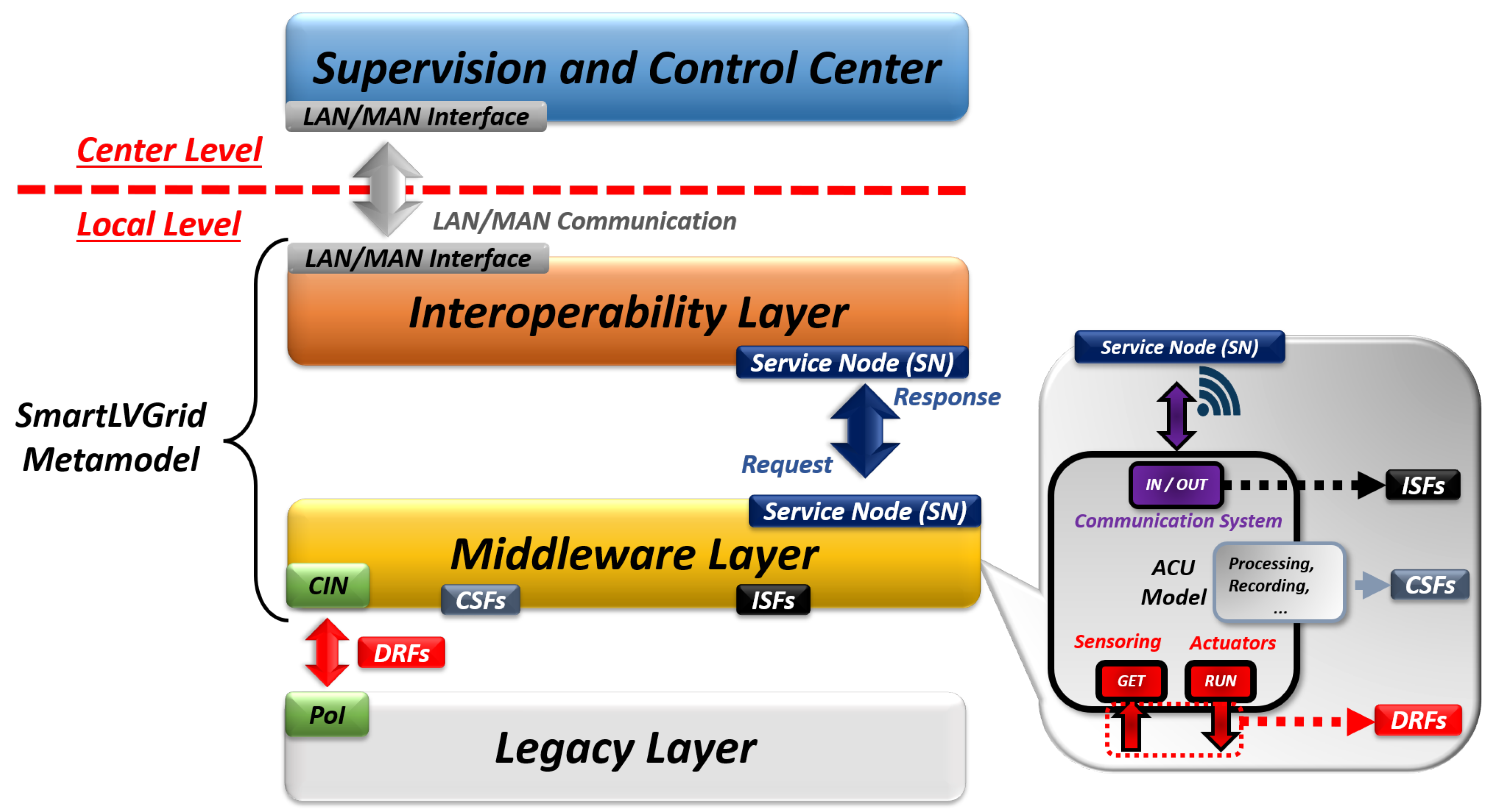
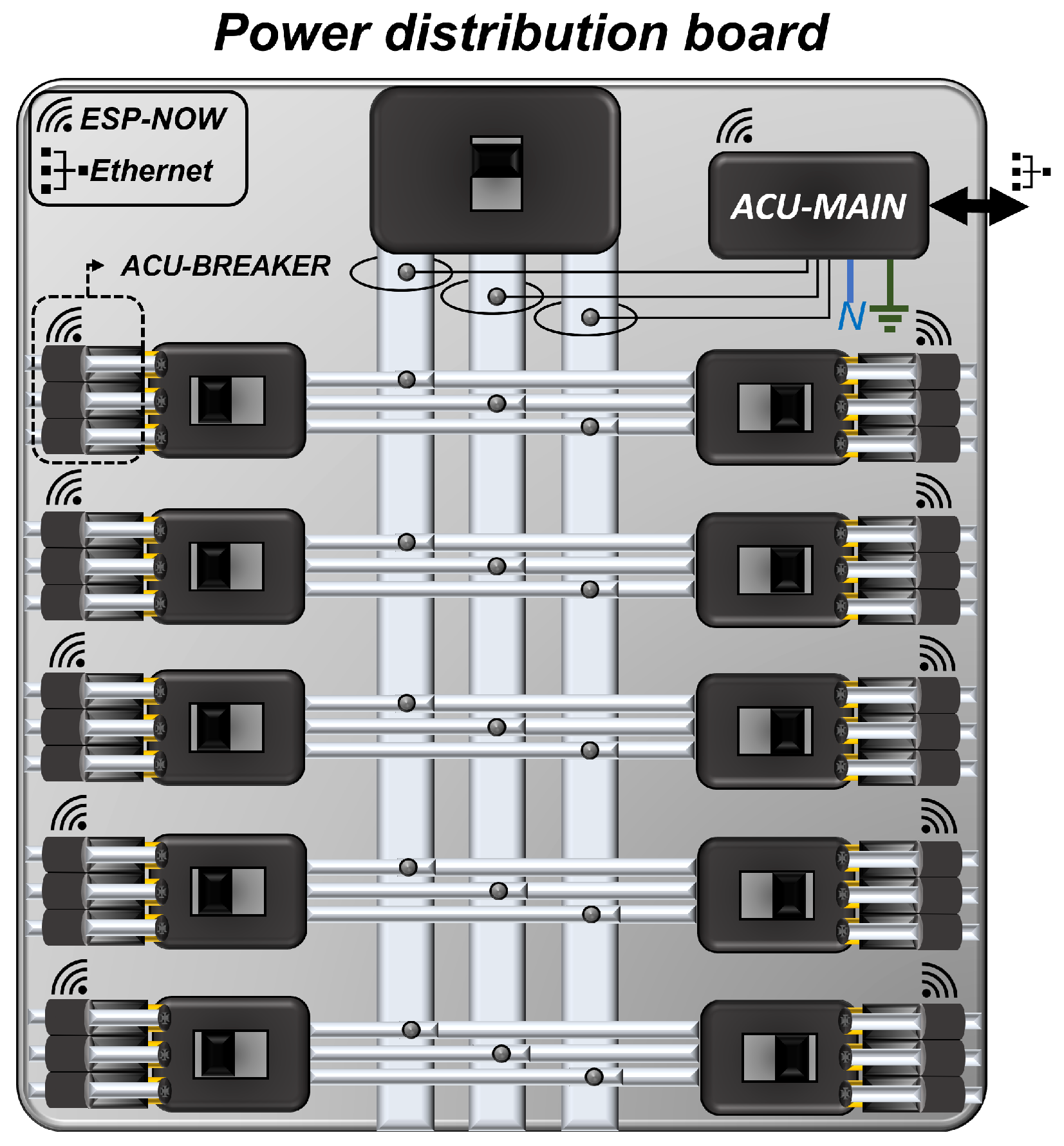
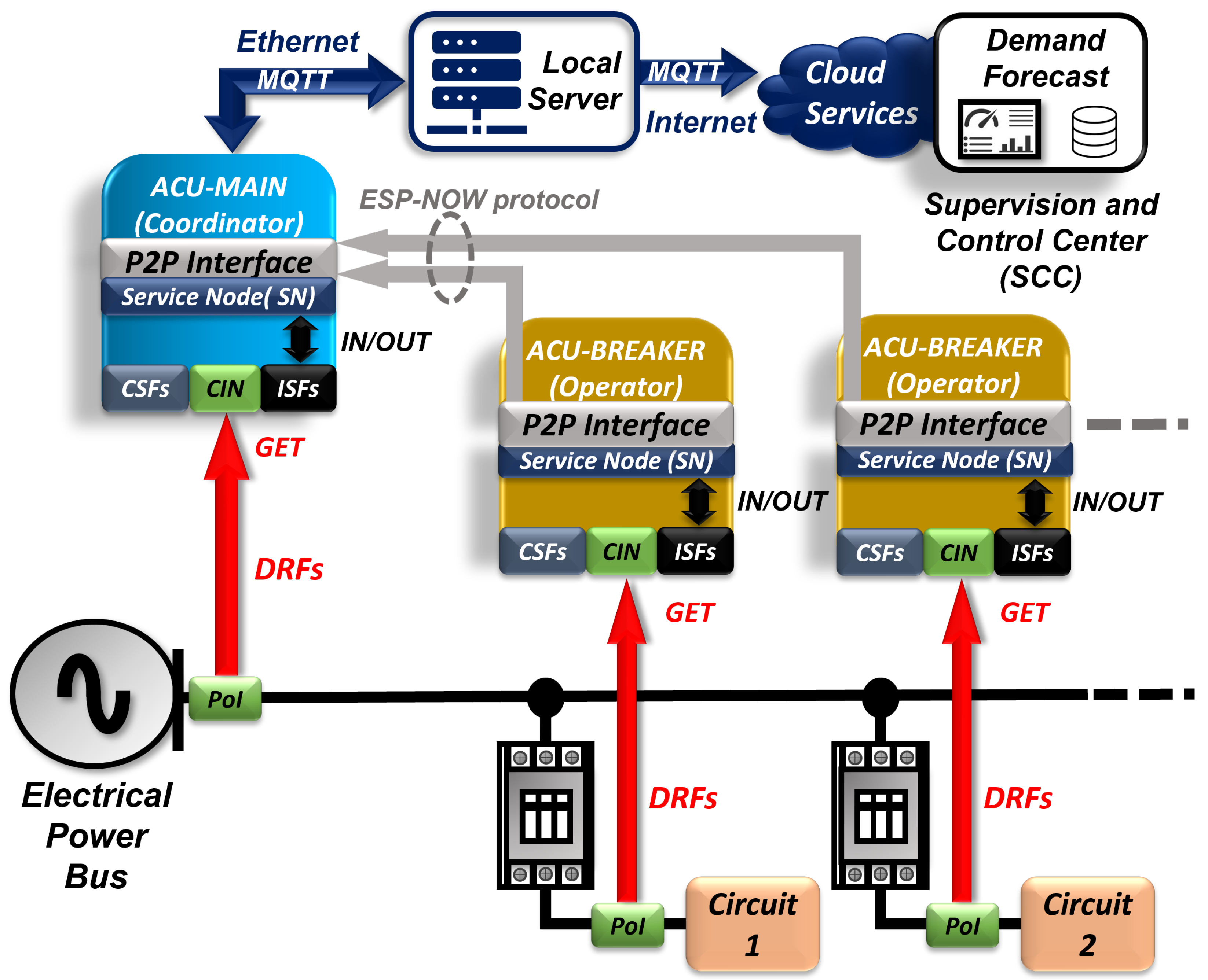
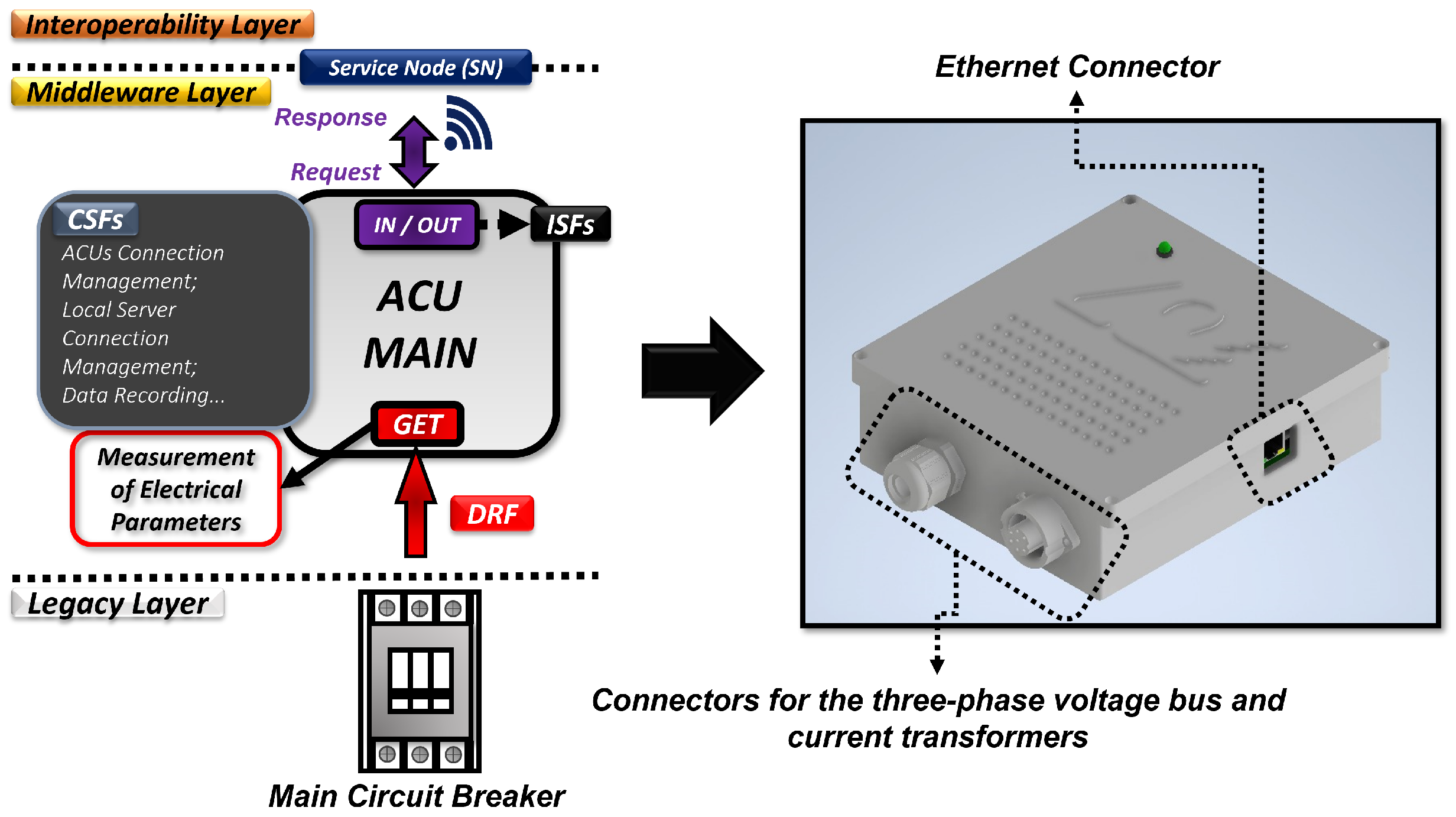
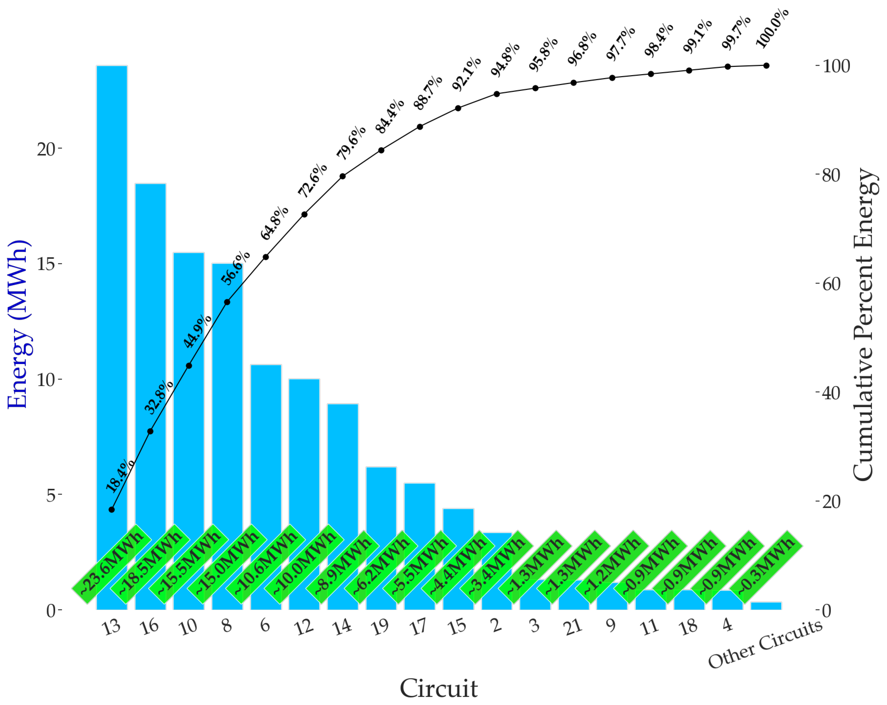
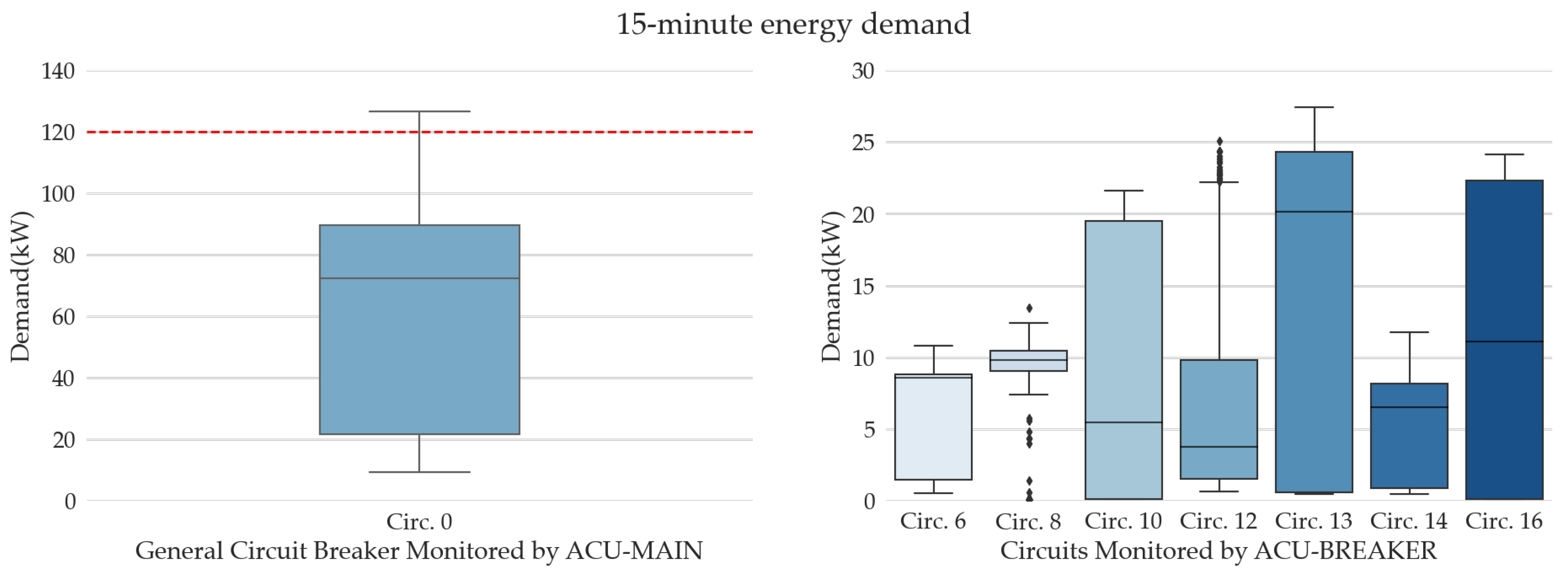