
Appraisal of Different Artificial Intelligence Techniques for the Prediction of Marble Strength

 , ,
, ,  , , and
Abstract
:1. Introduction
2. Materials and Methods
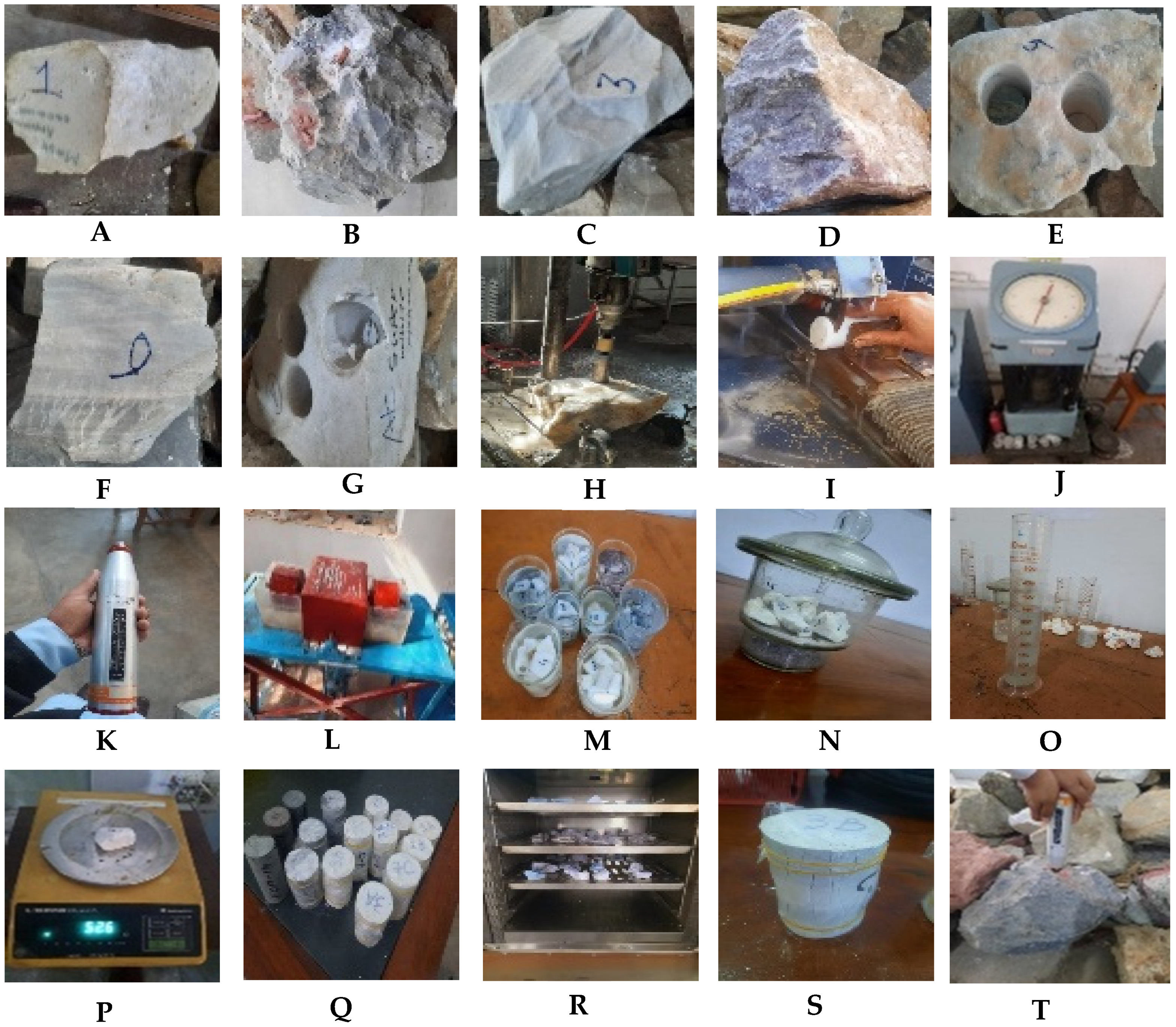
2.1. Design of Experimental Works
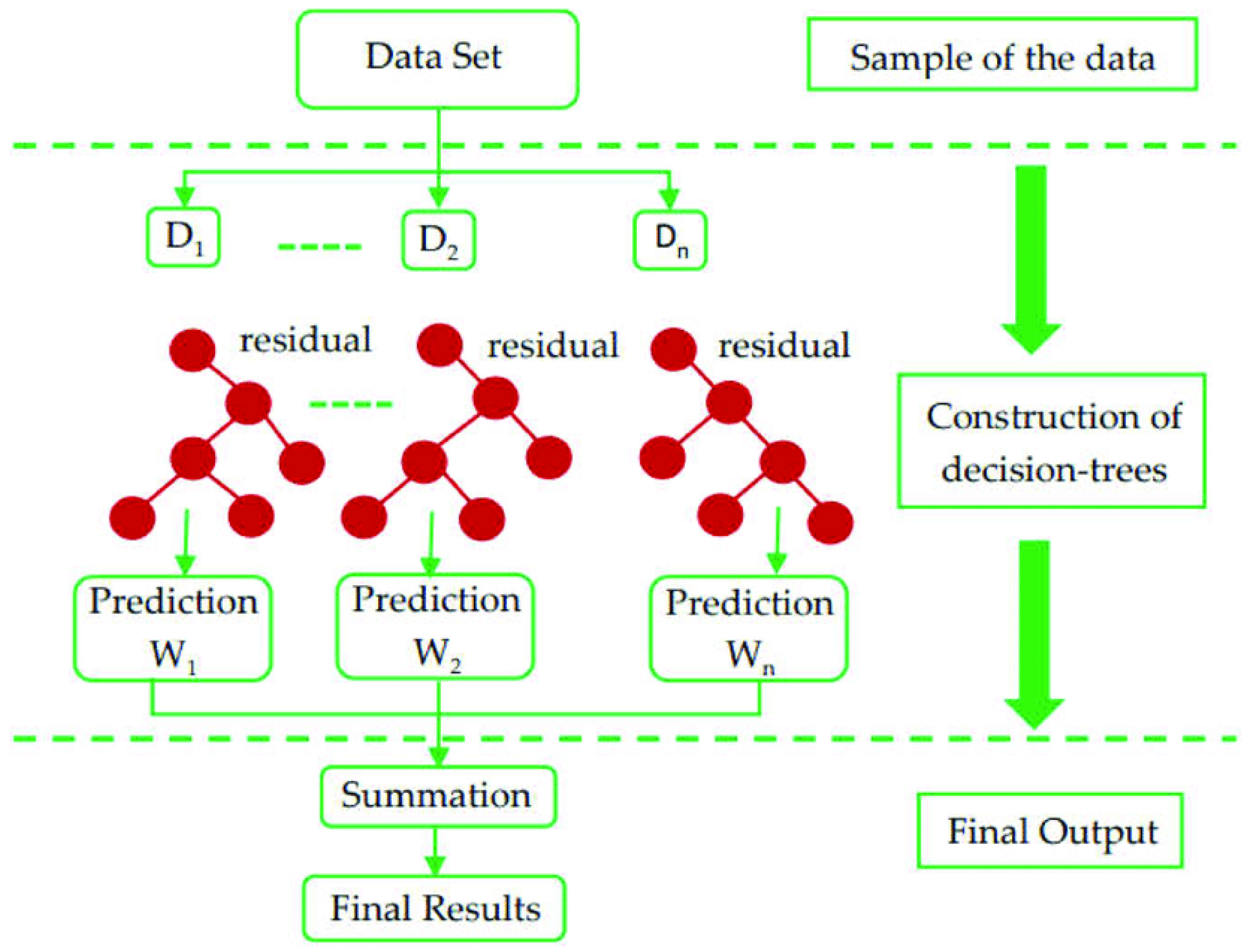
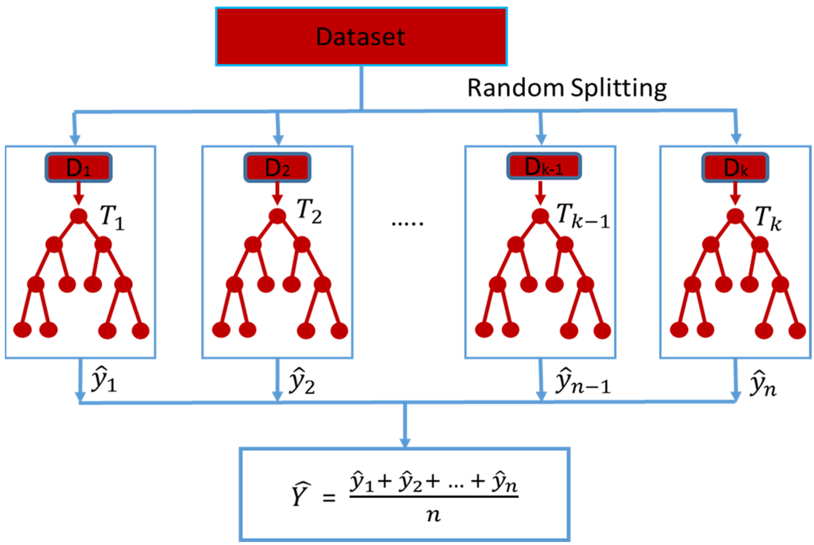
2.2. Predictive Models
- ;
- .
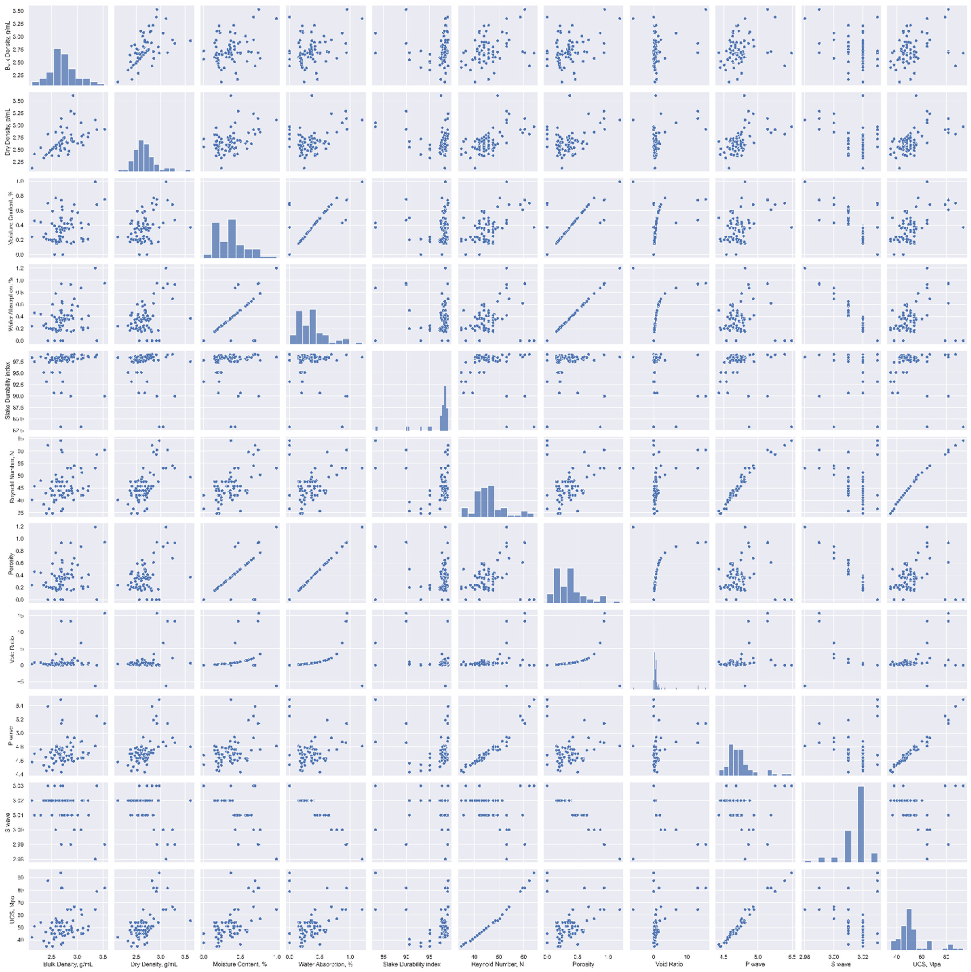
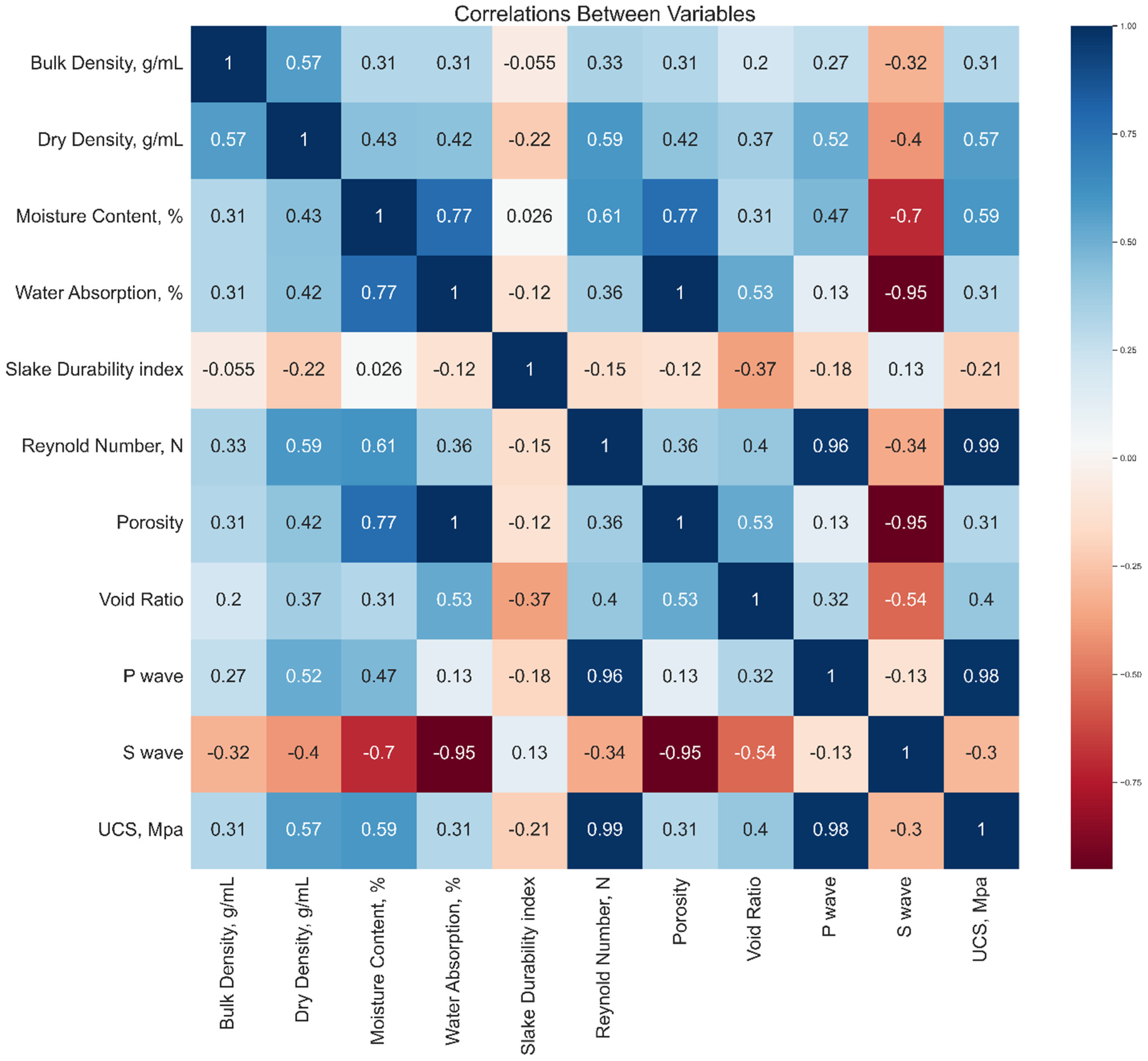
2.3. Data Analysis for Selecting the Most Appropriate Input Variables
2.4. Performance Indicator
- RSS = sum of the square of the residual;
- TSS = total sum of the square.
3. Analysis of Results
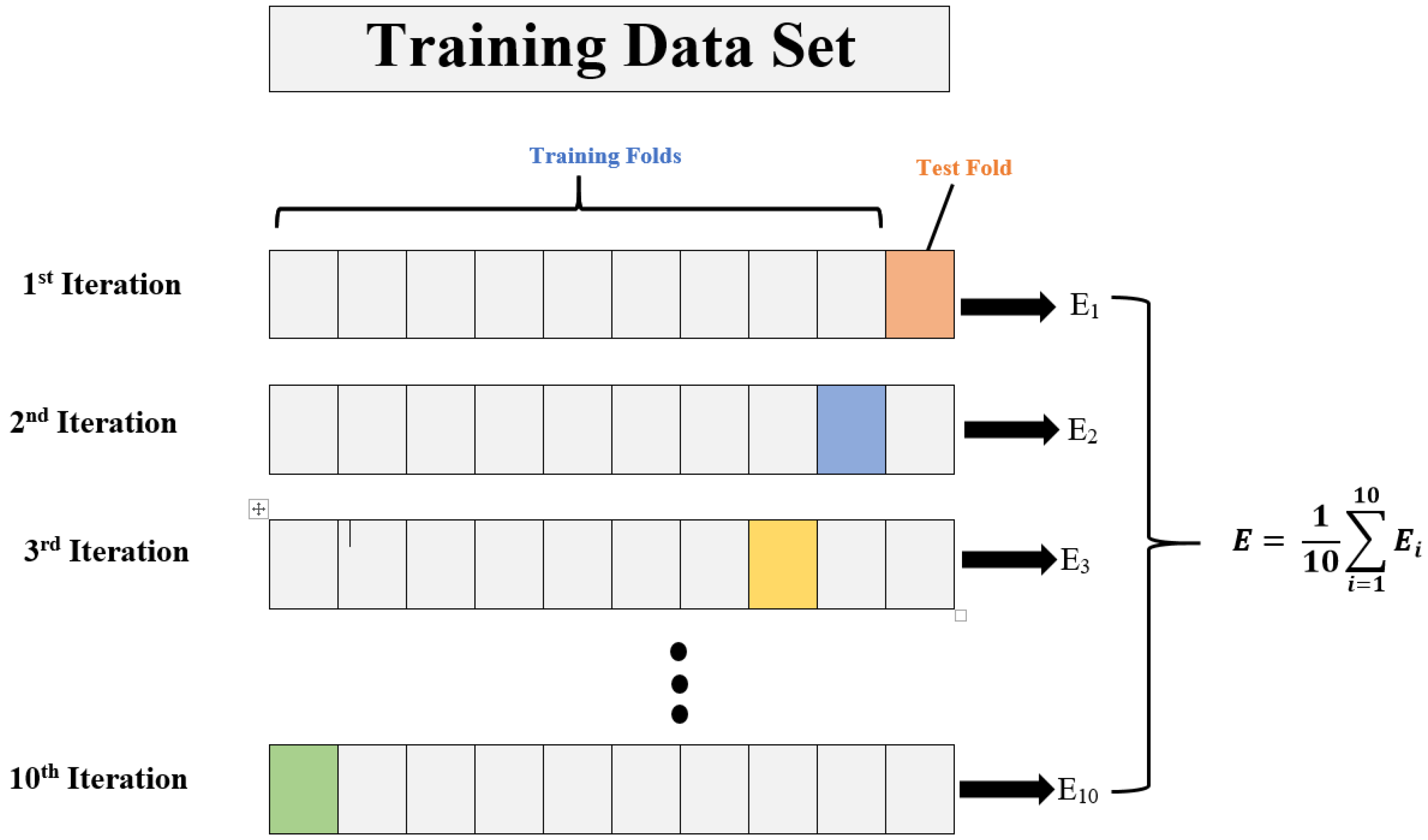
3.1. Model Hyperparameter Optimization
- In order to train the data set, the training data set needs to be divided into k folds.
- The (k˗-1) fold is used for training out of all k folds.
- The remaining last k-fold is used for validation.
- In order to train the model with specific hyperparameters, training data (k-1 folds) are used, and validation data are used as 1-fold. For each fold, the model’s performance is recorded.
- K-fold cross-validation refers to the process of repeating the steps above until each k-fold is used for validation purposes. That is why this process is known as “K-fold cross-validation”.
- After calculating each model score for each model in step d, the mean and standard deviation of the model performance are computed.
- It is necessary to repeat steps b to f for different values of the hyperparameters.
- The hyperparameters associated with the best mean and standard deviation of the model scores are then selected.
- Using the entire training data set, the model is trained, and its performance is evaluated on the basis of the test data set.
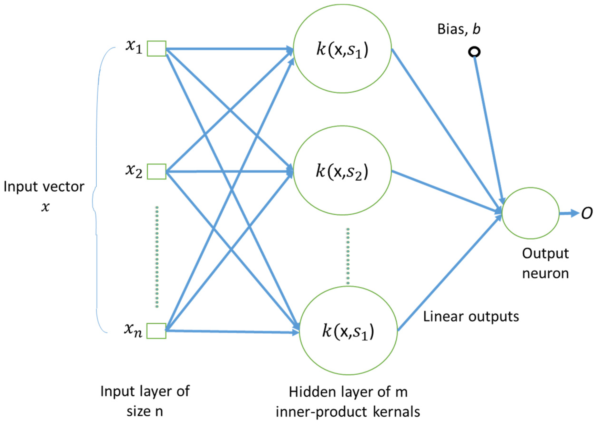
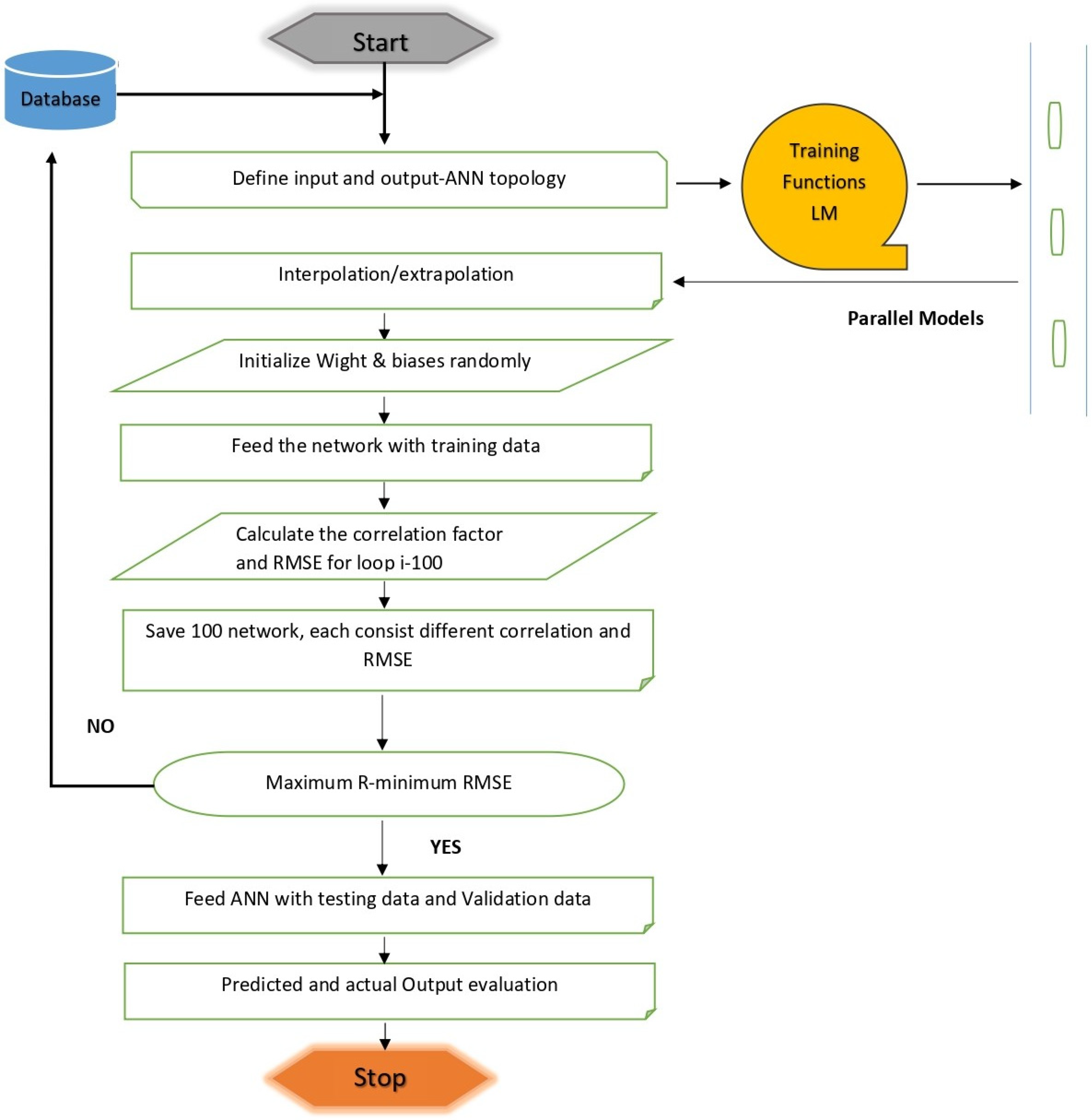
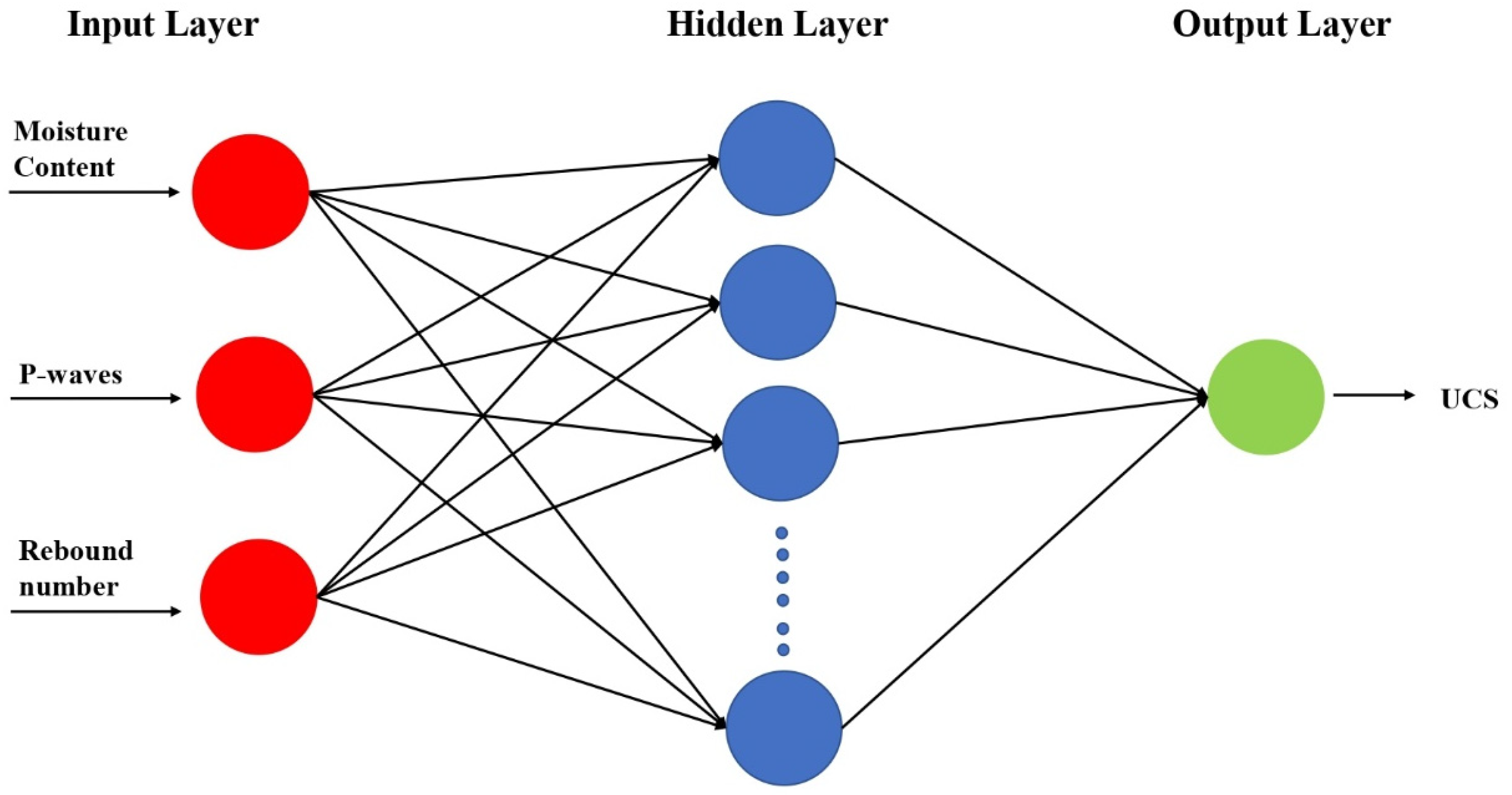
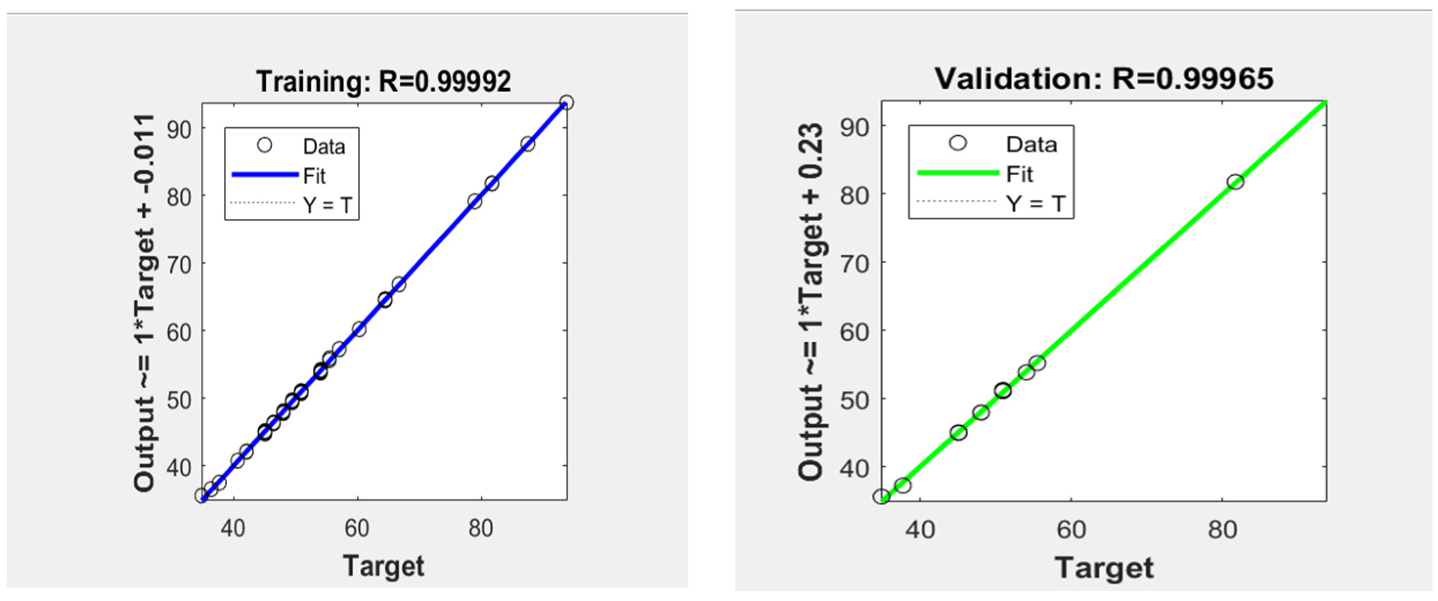
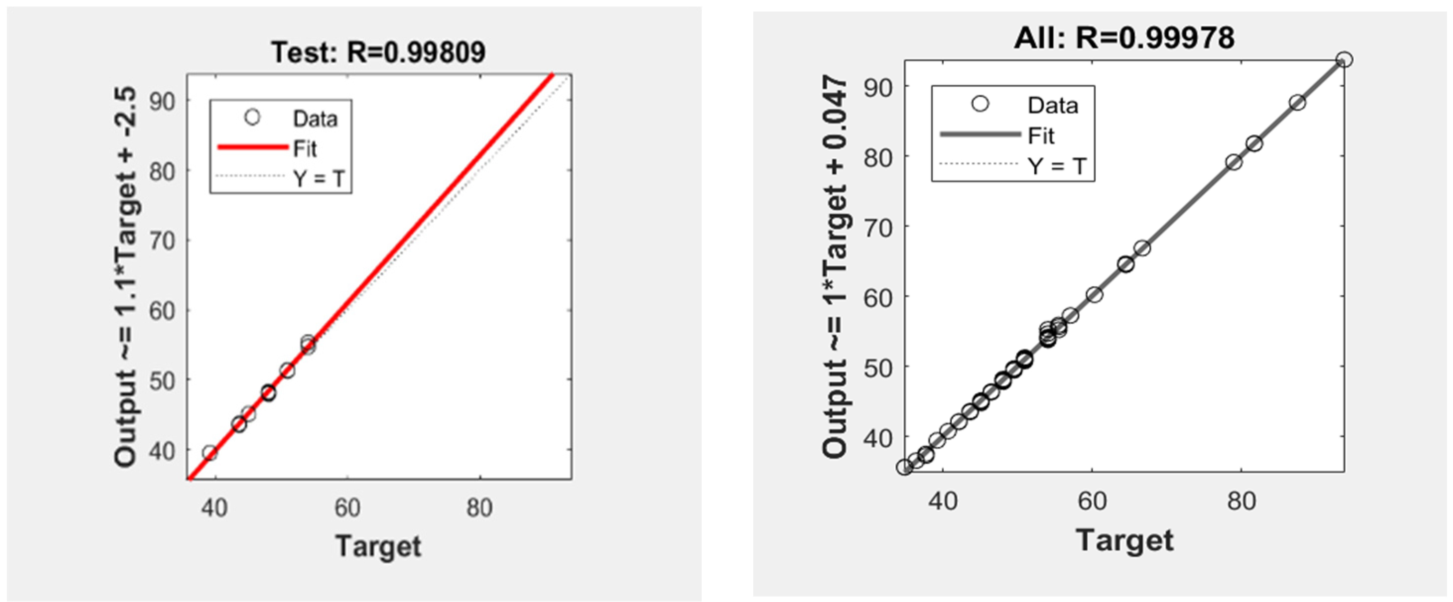
3.2. Prediction of UCS using Artificial Neural Networks
4. Discussion
5. Conclusions
Author Contributions
Funding
Institutional Review Board Statement
Informed Consent Statement
Data Availability Statement
Conflicts of Interest
References
- Dehghan, S.; Sattari, G.; Chelgani, S.C.; Aliabadi, M.J.M.S. Technology. Prediction of uniaxial compressive strength and modulus of elasticity for Travertine samples using regression and artificial neural networks. Min. Sci. Technol. 2010, 20, 41–46. [Google Scholar]
- Bieniawski, Z.T. Estimating the strength of rock materials. J. S. Afr. Inst. Min. Metall. 1974, 74, 312–320. [Google Scholar] [CrossRef]
- Mahdiabadi, N.; Khanlari, G.J. Prediction of uniaxial compressive strength and modulus of elasticity in calcareous mudstones using neural networks, fuzzy systems, and regression analysis. Period. Polytech. Civ. Eng. 2019, 63, 104–114. [Google Scholar] [CrossRef]
- Khan, N.M.; Cao, K.; Emad, M.Z.; Hussain, S.; Rehman, H.; Shah, K.S.; Rehman, F.U.; Muhammad, A.J. Development of Predictive Models for Determination of the Extent of Damage in Granite Caused by Thermal Treatment and Cooling Conditions Using Artificial Intelligence. Mathematics 2022, 10, 2883. [Google Scholar] [CrossRef]
- Wu, H.; Ju, Y.; Han, X.; Ren, Z.; Sun, Y.; Zhang, Y.; Han, T. Size effects in the uniaxial compressive properties of 3D printed models of rocks: An experimental investigation. Int. J. Coal Sci. Technol. 2022, 9, 83. [Google Scholar] [CrossRef]
- Gao, H.; Wang, Q.; Jiang, B.; Zhang, P.; Jiang, Z.; Wang, Y. Relationship between rock uniaxial compressive strength and digital core drilling parameters and its forecast method. Int. J. Coal Sci. Technol. 2021, 8, 605–613. [Google Scholar] [CrossRef]
- Kim, B.-H.; Walton, G.; Larson, M.K.; Berry, S. Investigation of the anisotropic confinement-dependent brittleness of a Utah coal. Int. J. Coal Sci. Technol. 2021, 8, 274–290. [Google Scholar] [CrossRef]
- Li, Y.; Mitri, H.S. Determination of mining-induced stresses using diametral rock core deformations. Int. J. Coal Sci. Technol. 2022, 9, 80. [Google Scholar] [CrossRef]
- Li, Y.; Yang, R.; Fang, S.; Lin, H.; Lu, S.; Zhu, Y.; Wang, M. Failure analysis and control measures of deep roadway with composite roof: A case study. Int. J. Coal Sci. Technol. 2022, 9, 2. [Google Scholar] [CrossRef]
- Liu, B.; Zhao, Y.; Zhang, C.; Zhou, J.; Li, Y.; Sun, Z. Characteristic strength and acoustic emission properties of weakly cemented sandstone at different depths under uniaxial compression. Int. J. Coal Sci. Technol. 2021, 8, 1288–1301. [Google Scholar] [CrossRef]
- Liu, T.; Lin, B.; Fu, X.; Liu, A. Mechanical criterion for coal and gas outburst: A perspective from multiphysics coupling. Int. J. Coal Sci. Technol. 2021, 8, 1423–1435. [Google Scholar] [CrossRef]
- Ma, D.; Duan, H.; Zhang, J.; Bai, H. A state-of-the-art review on rock seepage mechanism of water inrush disaster in coal mines. Int. J. Coal Sci. Technol. 2022, 9, 50. [Google Scholar] [CrossRef]
- Ulusay, R.; Hudson, J.A. The Complete ISRM Suggested Methods for Rock Characterization, Testing and Monitoring, 1974–2006; International Society for Rock Mechanics (ISRM): Ankara, Turkey; Pergamon, Turkey; Oxford, UK, 2007. [Google Scholar]
- Standard Test Method for Unconfined Compressive Strength of Intact Rock Core Specimens; ASTM 2938. ASTM International: West Conshohocken, PA, USA, 1995.
- Ali, Z.; Karakus, M.; Nguyen, G.D.; Amrouch, K. Effect of loading rate and time delay on the tangent modulus method (TMM) in coal and coal measured rocks. Int. J. Coal Sci. Technol. 2022, 9, 81. [Google Scholar] [CrossRef]
- Bai, Q.; Zhang, C.; Paul Young, R. Using true-triaxial stress path to simulate excavation-induced rock damage: A case study. Int. J. Coal Sci. Technol. 2022, 9, 49. [Google Scholar] [CrossRef]
- Chen, Y.; Zuo, J.; Liu, D.; Li, Y.; Wang, Z. Experimental and numerical study of coal-rock bimaterial composite bodies under triaxial compression. Int. J. Coal Sci. Technol. 2021, 8, 908–924. [Google Scholar] [CrossRef]
- Chi, X.; Yang, K.; Wei, Z. Breaking and mining-induced stress evolution of overlying strata in the working face of a steeply dipping coal seam. Int. J. Coal Sci. Technol. 2021, 8, 614–625. [Google Scholar] [CrossRef]
- Cavaleri, L.; Barkhordari, M.S.; Repapis, C.C.; Armaghani, D.J.; Ulrikh, D.V.; Asteris, P.G. Convolution-based ensemble learning algorithms to estimate the bond strength of the corroded reinforced concrete. Constr. Build. Mater. 2022, 359, 129504. [Google Scholar] [CrossRef]
- Ceryan, N. Application of support vector machines and relevance vector machines in predicting uniaxial compressive strength of volcanic rocks. J. Afr. Earth Sci. 2014, 100, 634–644. [Google Scholar] [CrossRef]
- Asadi, A. Application of artificial neural networks in prediction of uniaxial compressive strength of rocks using well logs and drilling data. Procedia Eng. 2017, 191, 279–286. [Google Scholar] [CrossRef]
- Skentou, A.D.; Bardhan, A.; Mamou, A.; Lemonis, M.E.; Kumar, G.; Samui, P.; Armaghani, D.J.; Asteris, P.G. Closed-Form Equation for Estimating Unconfined Compressive Strength of Granite from Three Non-destructive Tests Using Soft Computing Models. Rock Mech. Rock Eng. 2022, 56, 487–514. [Google Scholar] [CrossRef]
- Zhang, L.; Ding, X.; Budhu, M. A rock expert system for the evaluation of rock properties. Int. J. Rock Mech. Min. Sci. 2012, 50, 124–132. [Google Scholar] [CrossRef]
- Singh, T.N.; Verma, A.K. Comparative analysis of intelligent algorithms to correlate strength and petrographic properties of some schistose rocks. Eng. Comput. 2012, 28, 1–12. [Google Scholar] [CrossRef]
- Gokceoglu, C.; Sonmez, H.; Zorlu, K. Estimating the uniaxial compressive strength of some clay-bearing rocks selected from Turkey by nonlinear multivariable regression and rule-based fuzzy models. Expert Syst. 2009, 26, 176–190. [Google Scholar] [CrossRef]
- Sarkar, K.; Vishal, V.; Singh, T. An empirical correlation of index geomechanical parameters with the compressional wave velocity. Geotech. Geol. Eng. 2012, 30, 469–479. [Google Scholar] [CrossRef]
- Shan, F.; He, X.; Armaghani, D.J.; Zhang, P.; Sheng, D. Success and challenges in predicting TBM penetration rate using recurrent neural networks. Tunn. Undergr. Space Technol. 2022, 130, 104728. [Google Scholar] [CrossRef]
- Verwaal, W.; Mulder, A. Estimating rock strength with the Equotip hardness tester. Int. J. Rock Mech. Min. Sci. Geomech. Abstr. 1993, 30, 659–662. [Google Scholar] [CrossRef]
- Yagiz, S.; Sezer, E.; Gokceoglu, C. Artificial neural networks and nonlinear regression techniques to assess the influence of slake durability cycles on the prediction of uniaxial compressive strength and modulus of elasticity for carbonate rocks. Int. J. Numer. Anal. Methods Géoméch. 2012, 36, 1636–1650. [Google Scholar] [CrossRef]
- Grima, M.A.; Babuška, R. Fuzzy model for the prediction of unconfined compressive strength of rock samples. Int. J. Rock Mech. Min. Sci. 1999, 36, 339–349. [Google Scholar] [CrossRef]
- Indraratna, B.; Armaghani, D.J.; Correia, A.G.; Hunt, H.; Ngo, T. Prediction of resilient modulus of ballast under cyclic loading using machine learning techniques. Transp. Geotech. 2023, 38, 100895. [Google Scholar] [CrossRef]
- Feng, F.; Chen, S.; Zhao, X.; Li, D.; Wang, X.; Cui, J. Effects of external dynamic disturbances and structural plane on rock fracturing around deep underground cavern. Int. J. Coal Sci. Technol. 2022, 9, 15. [Google Scholar] [CrossRef]
- Gao, R.; Kuang, T.; Zhang, Y.; Zhang, W.; Quan, C. Controlling mine pressure by subjecting high-level hard rock strata to ground fracturing. Int. J. Coal Sci. Technol. 2021, 8, 1336–1350. [Google Scholar] [CrossRef]
- Gorai, A.K.; Raval, S.; Patel, A.K.; Chatterjee, S.; Gautam, T. Design and development of a machine vision system using artificial neural network-based algorithm for automated coal characterization. Int. J. Coal Sci. Technol. 2021, 8, 737–755. [Google Scholar] [CrossRef]
- He, S.; Qin, M.; Qiu, L.; Song, D.; Zhang, X. Early warning of coal dynamic disaster by precursor of AE and EMR “quiet period”. Int. J. Coal Sci. Technol. 2022, 9, 46. [Google Scholar] [CrossRef]
- Jangara, H.; Ozturk, C.A. Longwall top coal caving design for thick coal seam in very poor strength surrounding strata. Int. J. Coal Sci. Technol. 2021, 8, 641–658. [Google Scholar] [CrossRef]
- Nikolenko, P.V.; Epshtein, S.A.; Shkuratnik, V.L.; Anufrenkova, P.S. Experimental study of coal fracture dynamics under the influence of cyclic freezing–thawing using shear elastic waves. Int. J. Coal Sci. Technol. 2021, 8, 562–574. [Google Scholar] [CrossRef]
- Demir Sahin, D.; Isik, E.; Isik, I.; Cullu, M. Artificial neural network modeling for the effect of fly ash fineness on compressive strength. Arab. J. Geosci. 2021, 14, 2705. [Google Scholar] [CrossRef]
- Chen, S.; Xiang, Z.; Eker, H. Curing Stress Influences the Mechanical Characteristics of Cemented Paste Backfill and Its Damage Constitutive Model. Buildings 2022, 12, 1607. [Google Scholar] [CrossRef]
- Köken, E. Assessment of Los Angeles Abrasion Value (LAAV) and Magnesium Sulphate Soundness (Mwl) of Rock Aggregates Using Gene Expression Programming and Artificial Neural Networks. Arch. Min. Sci. 2022, 67, 401–422. [Google Scholar]
- Şahin, D.D.; Kumaş, C.; Eker, H. Research of the Use of Mine Tailings in Agriculture. JoCREST 2022, 8, 71–84. [Google Scholar]
- Strzałkowski, P.; Köken, E. Assessment of Böhme Abrasion Value of Natural Stones through Artificial Neural Networks (ANN). Materials 2022, 15, 2533. [Google Scholar] [CrossRef]
- Hussain, S.; Muhammad Khan, N.; Emad, M.Z.; Naji, A.M.; Cao, K.; Gao, Q.; Ur Rehman, Z.; Raza, S.; Cui, R.; Salman, M. An Appropriate Model for the Prediction of Rock Mass Deformation Modulus among Various Artificial Intelligence Models. Sustainability 2022, 14, 15225. [Google Scholar] [CrossRef]
- Chen, L.; Asteris, P.G.; Tsoukalas, M.Z.; Armaghani, D.J.; Ulrikh, D.V.; Yari, M. Forecast of Airblast Vibrations Induced by Blasting Using Support Vector Regression Optimized by the Grasshopper Optimization (SVR-GO) Technique. Appl. Sci. 2022, 12, 9805. [Google Scholar] [CrossRef]
- Zhou, J.; Lin, H.; Jin, H.; Li, S.; Yan, Z.; Huang, S. Cooperative prediction method of gas emission from mining face based on feature selection and machine learning. Int. J. Coal Sci. Technol. 2022, 9, 51. [Google Scholar] [CrossRef]
- Huang, F.; Xiong, H.; Chen, S.; Lv, Z.; Huang, J.; Chang, Z.; Catani, F. Slope stability prediction based on a long short-term memory neural network: Comparisons with convolutional neural networks, support vector machines and random forest models. Int. J. Coal Sci. Technol. 2023, 10, 18. [Google Scholar] [CrossRef]
- Vagnon, F.; Colombero, C.; Colombo, F.; Comina, C.; Ferrero, A.M.; Mandrone, G.; Vinciguerra, S.C. Effects of thermal treatment on physical and mechanical properties of Valdieri Marble-NW Italy. Int. J. Rock Mech. Min. Sci. 2019, 116, 75–86. [Google Scholar] [CrossRef]
- Manouchehrian, A.; Sharifzadeh, M.; Moghadam, R.H. Application of artificial neural networks and multivariate statistics to estimate UCS using textural characteristics. Int. J. Min. Sci. Technol. 2012, 22, 229–236. [Google Scholar] [CrossRef]
- Torabi-Kaveh, M.; Naseri, F.; Saneie, S.; Sarshari, B. Application of artificial neural networks and multivariate statistics to predict UCS and E using physical properties of Asmari limestones. Arab. J. Geosci. 2015, 8, 2889–2897. [Google Scholar] [CrossRef]
- Abdi, Y.; Garavand, A.T.; Sahamieh, R.Z. Prediction of strength parameters of sedimentary rocks using artificial neural networks and regression analysis. Arab. J. Geosci. 2018, 11, 587. [Google Scholar] [CrossRef]
- Prabakar, J.; Dendorkar, N.; Morchhale, R. Influence of fly ash on strength behavior of typical soils. Constr. Build. Mater. 2004, 18, 263–267. [Google Scholar] [CrossRef]
- Matin, S.; Farahzadi, L.; Makaremi, S.; Chelgani, S.C.; Sattari, G. Variable selection and prediction of uniaxial compressive strength and modulus of elasticity by random forest. Appl. Soft Comput. 2018, 70, 980–987. [Google Scholar] [CrossRef]
- Suthar, M. Applying several machine learning approaches for prediction of unconfined compressive strength of stabilized pond ashes. Neural Comput. Appl. 2020, 32, 9019–9028. [Google Scholar] [CrossRef]
- Wang, M.; Wan, W.; Zhao, Y. Prediction of the uniaxial compressive strength of rocks from simple index tests using a random forest predictive model. Comptes Rendus Mécanique 2020, 348, 3–32. [Google Scholar] [CrossRef]
- Ren, Q.; Wang, G.; Li, M.; Han, S. Prediction of rock compressive strength using machine learning algorithms based on spectrum analysis of geological hammer. Geotech. Geol. Eng. 2019, 37, 475–489. [Google Scholar] [CrossRef]
- Ghasemi, E.; Kalhori, H.; Bagherpour, R.; Yagiz, S. Model tree approach for predicting uniaxial compressive strength and Young’s modulus of carbonate rocks. Bull. Eng. Geol. Environ. 2018, 77, 331–343. [Google Scholar] [CrossRef]
- Saedi, B.; Mohammadi, S.D. Prediction of uniaxial compressive strength and elastic modulus of migmatites by microstructural characteristics using artificial neural networks. Rock Mech. Rock Eng. 2021, 54, 5617–5637. [Google Scholar] [CrossRef]
- Shahani, N.M.; Zheng, X.; Liu, C.; Hassan, F.U.; Li, P. Developing an XGBoost regression model for predicting young’s modulus of intact sedimentary rocks for the stability of surface and subsurface structures. Front. Earth Sci. 2021, 9, 761990. [Google Scholar] [CrossRef]
- Armaghani, D.J.; Tonnizam Mohamad, E.; Momeni, E.; Monjezi, M.; Sundaram Narayanasamy, M.S. Prediction of the strength and elasticity modulus of granite through an expert artificial neural network. Arab. J. Geosci. 2016, 9, 48. [Google Scholar] [CrossRef]
- Fairhurst, C.; Hudson, J.A. Draft ISRM suggested method for the complete stress-strain curve for intact rock in uniaxial compression. Int. J. Rock Mech. Min. Sci. Geomech. Abstr. 1999, 36, 279–289. [Google Scholar]
- Małkowski, P.; Niedbalski, Z.; Balarabe, T. A statistical analysis of geomechanical data and its effect on rock mass numerical modeling: A case study. Int. J. Coal Sci. Technol. 2021, 8, 312–323. [Google Scholar] [CrossRef]
- Ramraj, S.; Uzir, N.; Sunil, R.; Banerjee, S. Experimenting XGBoost algorithm for prediction and classification of different datasets. Int. J. Control. Theory Appl. 2016, 9, 651–662. [Google Scholar]
- Chandrahas, N.S.; Choudhary, B.S.; Teja, M.V.; Venkataramayya, M.; Prasad, N.K. XG Boost Algorithm to Simultaneous Prediction of Rock Fragmentation and Induced Ground Vibration Using Unique Blast Data. Appl. Sci. 2022, 12, 5269. [Google Scholar] [CrossRef]
- Shahani, N.M.; Zheng, X.; Guo, X.; Wei, X. Machine learning-based intelligent prediction of elastic modulus of rocks at thar coalfield. Sustainability 2022, 14, 3689. [Google Scholar] [CrossRef]
- Choi, H.-y.; Cho, K.-H.; Jin, C.; Lee, J.; Kim, T.-H.; Jung, W.-S.; Moon, S.-K.; Ko, C.-N.; Cho, S.-Y.; Jeon, C.-Y. Exercise therapies for Parkinson’s disease: A systematic review and meta-analysis. Park. Dis. 2020, 2020, 2565320. [Google Scholar] [CrossRef] [PubMed]
- Ogunkunle, T.F.; Okoro, E.E.; Rotimi, O.J.; Igbinedion, P.; Olatunji, D.I. Artificial intelligence model for predicting geomechanical characteristics using easy-to-acquire offset logs without deploying logging tools. Petroleum 2022, 8, 192–203. [Google Scholar] [CrossRef]
- Yang, Z.; Wu, Y.; Zhou, Y.; Tang, H.; Fu, S. Assessment of machine learning models for the prediction of rate-dependent compressive strength of rocks. Minerals 2022, 12, 731. [Google Scholar] [CrossRef]
- Gu, J.-C.; Lee, S.-C.; Suh, Y.-H. Determinants of behavioral intention to mobile banking. J. Agric. Food Res. 2009, 36, 11605–11616. [Google Scholar] [CrossRef]
- Qin, P.; Wang, T.; Luo, Y. A review on plant-based proteins from soybean: Health benefits and soy product development. J. Agric. Food Res. 2022, 7, 100265. [Google Scholar] [CrossRef]
- Frimpong, E.A.; Okyere, P.Y.; Asumadu, J. Prediction of transient stability status using Walsh-Hadamard transform and support vector machine. In Proceedings of the 2017 IEEE PES PowerAfrica, Accra, Ghana, 27–30 June 2017; pp. 301–306. [Google Scholar]
- Hassan, M.Y.; Arman, H. Comparison of six machine-learning methods for predicting the tensile strength (Brazilian) of evaporitic rocks. Appl. Sci. 2021, 11, 5207. [Google Scholar] [CrossRef]
- Ogutu, J.O.; Schulz-Streeck, T.; Piepho, H.-P. Genomic selection using regularized linear regression models: Ridge regression, lasso, elastic net and their extensions. BMC Proc. 2012, 6, S10. [Google Scholar] [CrossRef]
- Ozanne, M.; Dyar, M.; Carmosino, M.; Breves, E.; Clegg, S.; Wiens, R. Comparison of lasso and elastic net regression for major element analysis of rocks using laser-induced breakdown spectroscopy (LIBS). In Proceedings of the 43rd Annual Lunar and Planetary Science Conference, The Woodlands, TX, USA, 19–23 March 2012; p. 2391. [Google Scholar]
- Sarkar, K.; Tiwary, A.; Singh, T. Estimation of strength parameters of rock using artificial neural networks. Bull. Eng. Geol. Environ. 2010, 69, 599–606. [Google Scholar] [CrossRef]
- Tayarani, N.S.; Jamali, S.; Zadeh, M.M. Combination of artificial neural networks and numerical modeling for predicting deformation modulus of rock masses. Arch. Min. Sci. 2020, 65, 337–346. [Google Scholar]
- Lawal, A.I.; Kwon, S.J. Application of artificial intelligence to rock mechanics: An overview. J. Rock Mech. Geotech. Eng. 2021, 13, 248–266. [Google Scholar] [CrossRef]
- Ma, L.; Khan, N.M.; Cao, K.; Rehman, H.; Salman, S.; Rehman, F.U. Prediction of Sandstone Dilatancy Point in Different Water Contents Using Infrared Radiation Characteristic: Experimental and Machine Learning Approaches. Lithosphere 2022, 2021, 3243070. [Google Scholar] [CrossRef]
- Khan, N.M.; Ma, L.; Cao, K.; Hussain, S.; Liu, W.; Xu, Y. Infrared radiation characteristics based rock failure indicator index for acidic mudstone under uniaxial loading. Arab. J. Geosci. 2022, 15, 343. [Google Scholar] [CrossRef]
- Kutty, A.A.; Wakjira, T.G.; Kucukvar, M.; Abdella, G.M.; Onat, N.C. Urban resilience and livability performance of European smart cities: A novel machine learning approach. J. Clean. Prod. 2022, 378, 134203. [Google Scholar] [CrossRef]
- Bekdaş, G.; Cakiroglu, C.; Kim, S.; Geem, Z.W. Optimal dimensioning of retaining walls using explainable ensemble learning algorithms. Materials 2022, 15, 4993. [Google Scholar] [CrossRef]


| S.No | Input and Output | N total | Mean | Standard Deviation | Sum | Min | Median | Max |
|---|---|---|---|---|---|---|---|---|
| 1 | bulk density (g/mL) | 70.00 | 2.73 | 0.27 | 191.34 | 2.12 | 2.69 | 3.53 |
| 2 | dry density (g/mL) | 70.00 | 2.67 | 0.24 | 187.16 | 2.12 | 2.65 | 3.61 |
| 3 | moisture content (MC (%)) | 70.00 | 0.36 | 0.19 | 25.46 | 0.00 | 0.35 | 0.99 |
| 4 | water absorption (%) | 70.00 | 0.36 | 0.24 | 25.28 | 0.00 | 0.34 | 1.20 |
| 5 | slake durability index (Id2) | 70.00 | 97.08 | 3.21 | 6795.85 | 83.24 | 98.25 | 99.11 |
| 6 | rebound number (R) | 70.00 | 45.88 | 6.31 | 3211.57 | 34.70 | 44.82 | 64.14 |
| 7 | porosity (η) | 70.00 | 0.36 | 0.24 | 25.28 | 0.00 | 0.34 | 1.20 |
| 8 | void ratio (e) | 70.00 | 1.15 | 3.03 | 80.25 | 0.00 | 0.0034 | 0.012 |
| 9 | P-wave (km/s) | 70.00 | 4.74 | 0.20 | 331.52 | 4.43 | 4.70 | 5.49 |
| 10 | S-wave (km/s) | 70.00 | 3.02 | 0.01 | 211.14 | 2.98 | 3.02 | 3.03 |
| 11 | UCS (Mpa) | 70.00 | 52.17 | 12.10 | 3651.59 | 34.89 | 49.51 | 93.76 |
| Output | Model | Parameters |
|---|---|---|
| UCS (Mpa) | Artificial Neural Network | Neuron = 48 |
| XG Boost Regressor | learning_rate = 0.01, max_depth = 3, n_estimators = 100 | |
| Support Vector Machine | n_split = 10, n_repeats = 5, random state = 42, C = 1 function = SVR (kernal ‘rbf’) | |
| Random Forest Regression | n_split = 10, n_repeats = 5, random state = 42, max_depth = 3 | |
| Lasso | Alpha = 0.01, n_split = 10, n_repeats = 5, random state = 42 | |
| Elastic Net | Alpha = 0.01, l1_ratio = 0.95, n_split = 10, n_repeats = 5, random state = 42 | |
| Ridge | Alpha = 0.1, n_split = 10, n_repeats = 5, random state = 42 |
| S.no | Models | Training Accuracy | Testing Accuracy | ||||||
|---|---|---|---|---|---|---|---|---|---|
| R2 | MAE | MSE | RMSE | R2 | MAE | MSE | RMSE | ||
| 1 | Artificial Neural Network | 0.9990 | 0.1428 | 0.0782 | 0.2796 | 0.9995 | 0.1642 | 0.0694 | 0.2634 |
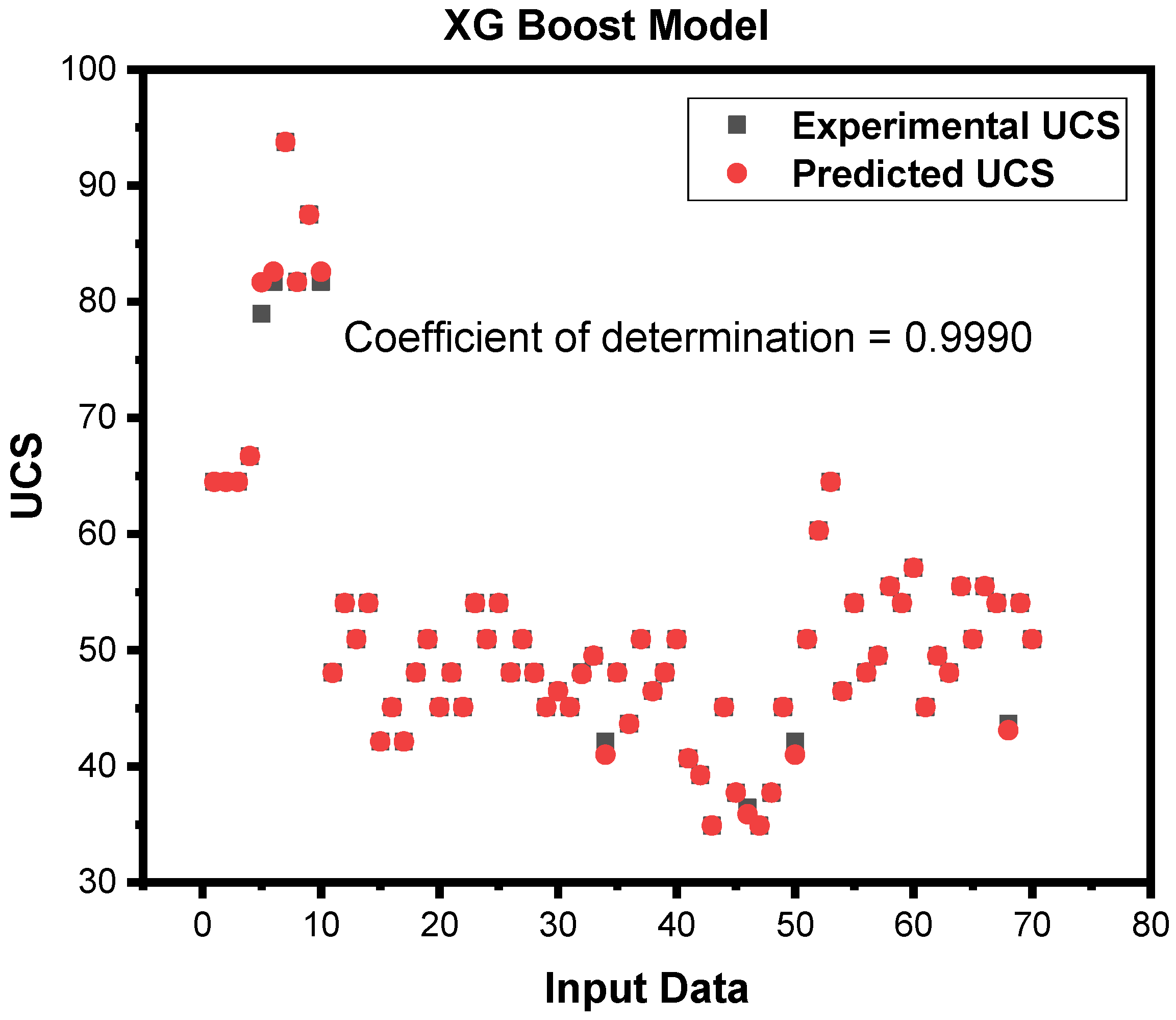
| 2 | XG Boost Regressor | 0.9989 | 0.5694 | 0.8664 | 0.9308 | 0.9990 | 0.1145 | 0.1732 | 0.4162 |
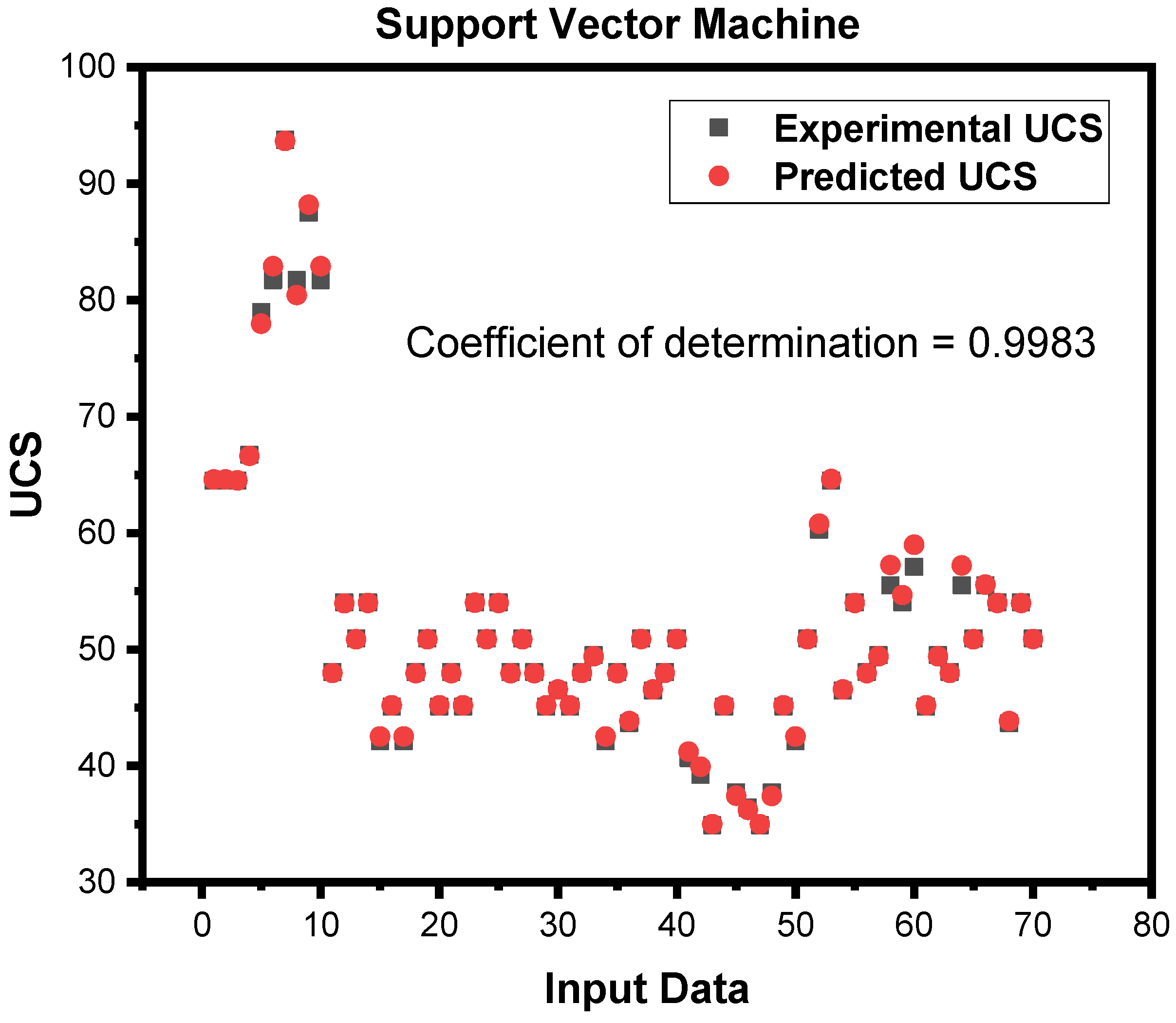
| 3 | Support Vector Machine | 0.9987 | 0.3649 | 0.3022 | 0.5498 | 0.9983 | 0.2891 | 0.2595 | 0.5094 |
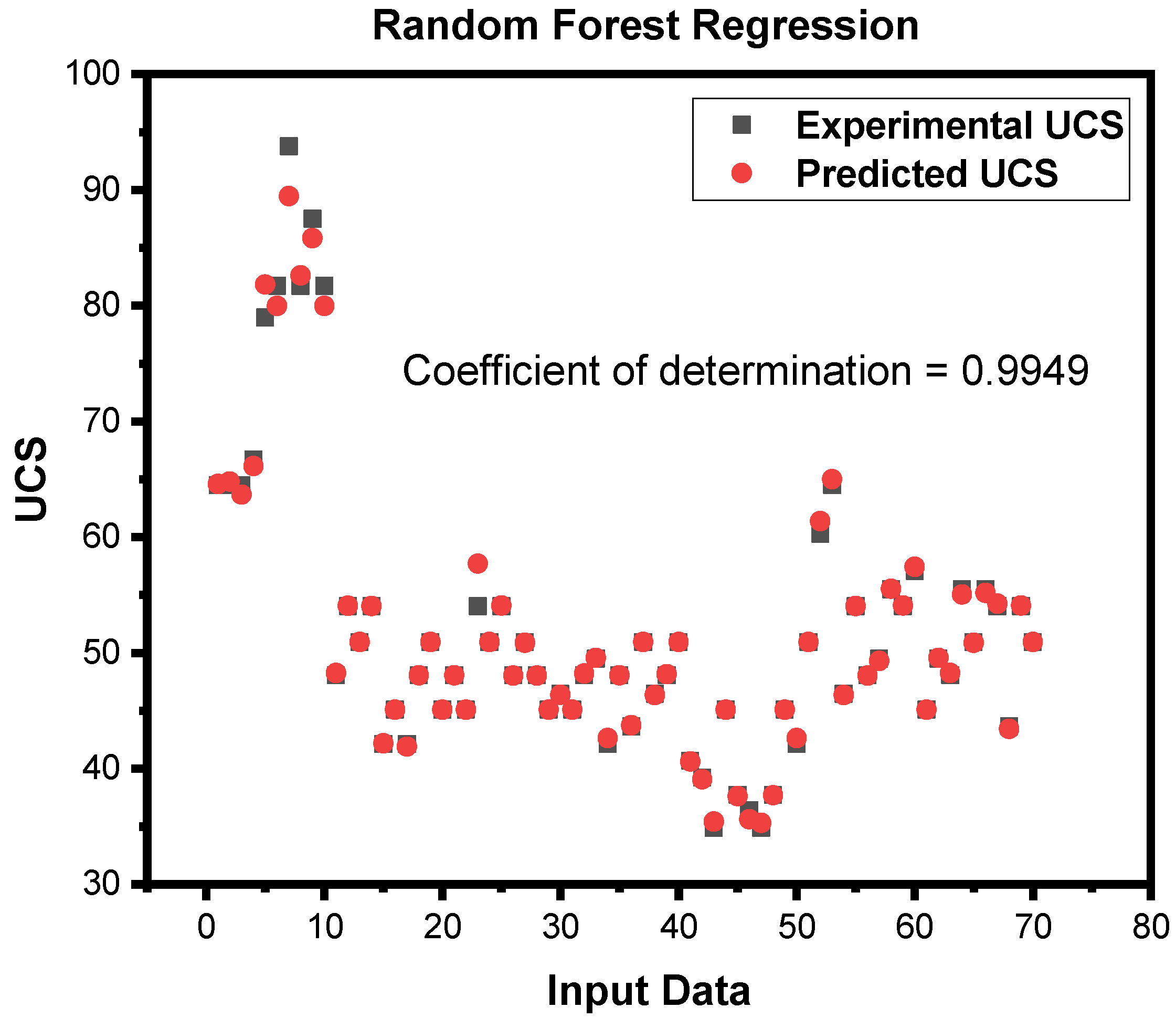
| 4 | Random Forest Regression | 0.9943 | 0.7176 | 1.3294 | 1.1530 | 0.9949 | 0.3555 | 0.6584 | 0.8114 |
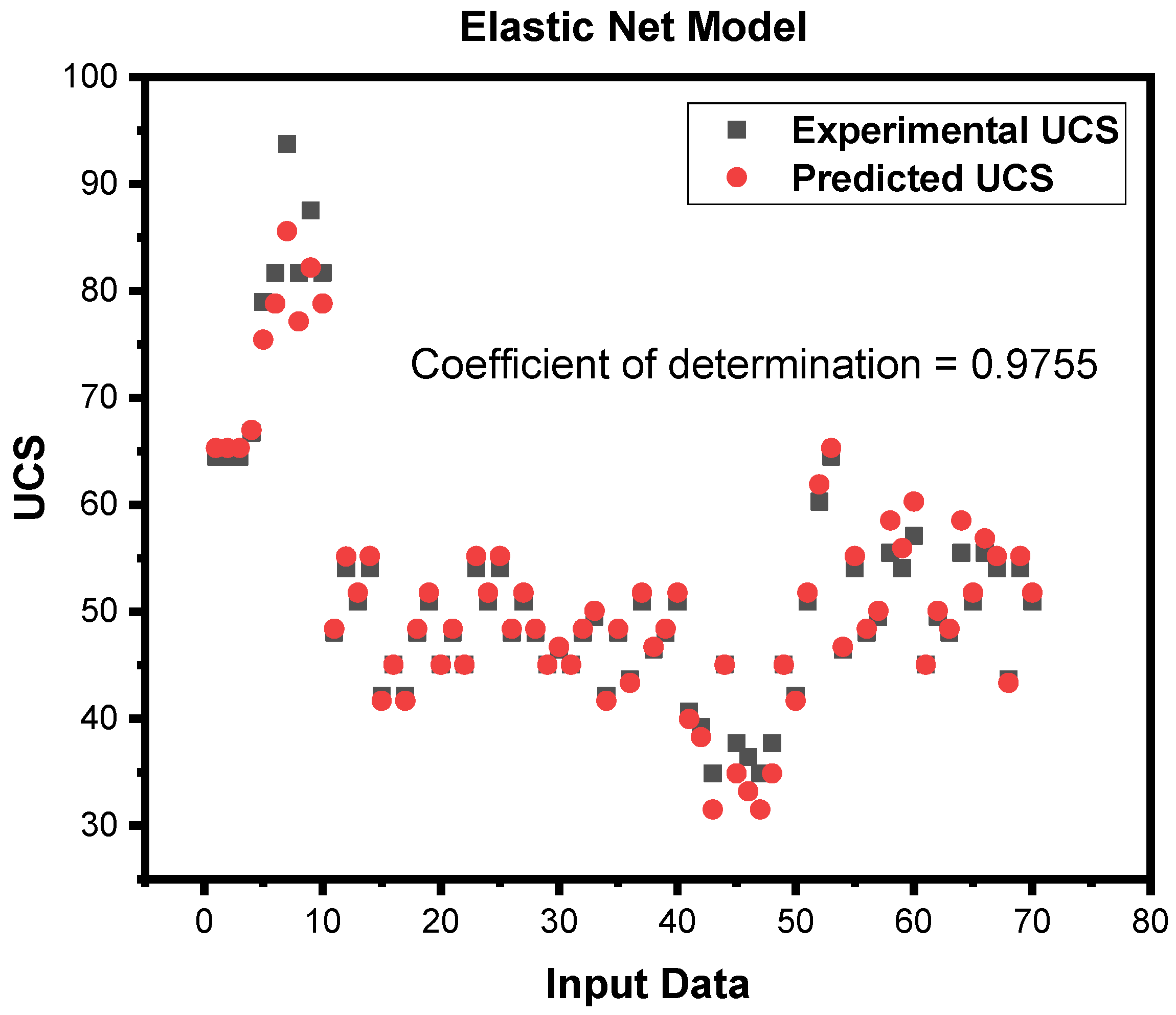
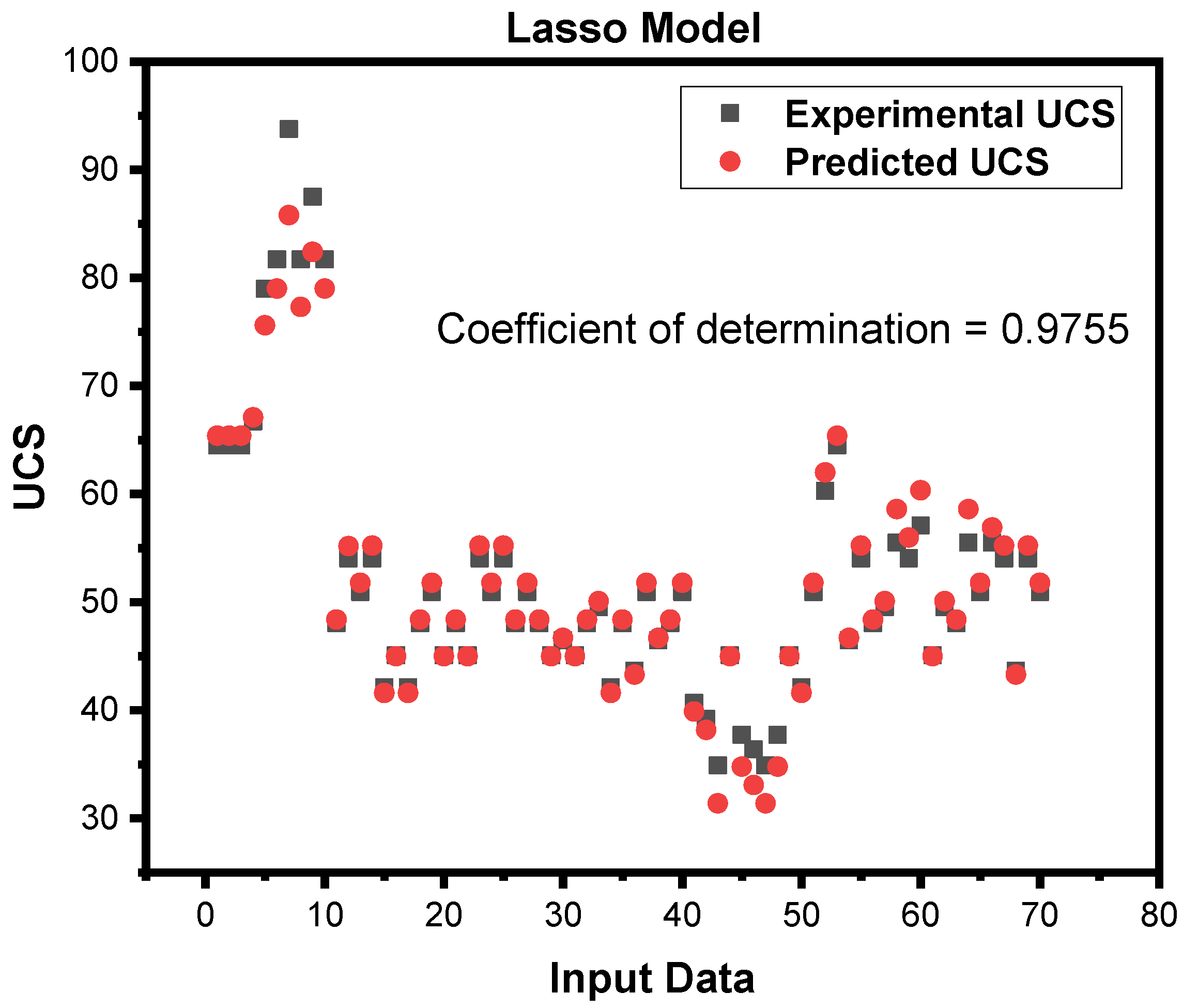
| 5 | Lasso | 0.9887 | 1.3670 | 3.0666 | 1.7512 | 0.9755 | 1.8918 | 3.5788 | 1.2555 |
| 6 | Elastic Net | 0.9887 | 1.3751 | 3.2071 | 1.7908 | 0.9755 | 1.2410 | 3.6308 | 1.9055 |
| 7 | Ridge | 0.9876 | 1.3906 | 3.0492 | 1.7462 | 0.9790 | 1.2149 | 3.0010 | 1.7347 |
Disclaimer/Publisher’s Note: The statements, opinions and data contained in all publications are solely those of the individual author(s) and contributor(s) and not of MDPI and/or the editor(s). MDPI and/or the editor(s) disclaim responsibility for any injury to people or property resulting from any ideas, methods, instructions or products referred to in the content. |
© 2023 by the authors. Licensee MDPI, Basel, Switzerland. This article is an open access article distributed under the terms and conditions of the Creative Commons Attribution (CC BY) license (https://creativecommons.org/licenses/by/4.0/).
Share and Cite
Jan, M.S.; Hussain, S.; e Zahra, R.; Emad, M.Z.; Khan, N.M.; Rehman, Z.U.; Cao, K.; Alarifi, S.S.; Raza, S.; Sherin, S.; et al. Appraisal of Different Artificial Intelligence Techniques for the Prediction of Marble Strength. Sustainability 2023, 15, 8835. https://doi.org/10.3390/su15118835
Jan MS, Hussain S, e Zahra R, Emad MZ, Khan NM, Rehman ZU, Cao K, Alarifi SS, Raza S, Sherin S, et al. Appraisal of Different Artificial Intelligence Techniques for the Prediction of Marble Strength. Sustainability. 2023; 15(11):8835. https://doi.org/10.3390/su15118835
Chicago/Turabian StyleJan, Muhammad Saqib, Sajjad Hussain, Rida e Zahra, Muhammad Zaka Emad, Naseer Muhammad Khan, Zahid Ur Rehman, Kewang Cao, Saad S. Alarifi, Salim Raza, Saira Sherin, and et al. 2023. "Appraisal of Different Artificial Intelligence Techniques for the Prediction of Marble Strength" Sustainability 15, no. 11: 8835. https://doi.org/10.3390/su15118835