1. Introduction
Studying pedestrian flow dynamics is essential for understanding how people move through various public spaces. This knowledge is crucial for designing safer and more efficient transportation systems and urban environments [
1,
2,
3,
4,
5]. By analyzing pedestrian behaviors, researchers and urban planners can optimize walking paths, and develop effective strategies to manage crowds during large events or emergencies [
6,
7,
8,
9,
10]. This work can be very helpful for sustainable transportation.
Among many useful topics in the field of pedestrian flow, single-file flow is very important since it is a fundamental aspect of pedestrian flow in a variety of settings. Such flow can be observed in many places, including narrow pathways or sidewalks, staircases, mountain trails, emergency exits or evacuation routes, etc. In particular, it can sometimes be found on the temporary paths near construction zones. Therefore, the study of single-file pedestrian flow may be helpful for many aspects, including the design of sustainable pedestrian infrastructure, the control strategies of pedestrian flow and the management of pedestrian evacuations in certain environments, etc.
In recent times, researchers have carried out several studies on this topic. For example, Cao et al. [
11] found that the sensitivity of pedestrians to changes in crowd density is related to visibility. Ren et al. [
12] found that, compared to the young, elderly persons are more sensitive to headway while adapting their speeds. This study can help to improve the pedestrian model for the elderly. Wang et al. [
13] focused on the microscopic characteristics of single-file flow on campuses, and the results indicated that the influence of age and gender were significant to speed, time–headway, and swaying amplitude. Lu et al. [
14] uncovered the characteristics of pedestrian movement under different social distancing measures. Xue et al. [
15] investigated the one-dimensional leader–follower behavior of children. The study found that the revealed characteristic delay time of children depends on densities. Ye et al. [
16] conducted single-file flow experiments on stairs at various densities. The study found that pedestrians who have a higher motivation have a stronger ability to adapt their velocities. In addition, the topic of gender influence is discussed by Subaih et al. [
17] and Dias et al. [
18]. Subaih et al. [
17] found that the mean velocity of exclusively male pedestrians is approximately the same as exclusively female pedestrians, thus there is no gender difference in pedestrian movement behavior. On the contrary, the outcomes of Dias et al. [
18] revealed that, in addition to relative speed, gender has a significant influence on instantaneous acceleration and deceleration for all density levels. Such contrast implies that further details on the influence of gender need to be investigated in the future.
Although many findings from different perspectives have been presented in these papers, the main deficiency of them is that the consideration of high-density conditions is lacking. As shown in
Table 1, in all the studies, the maximum density considered is no more than 2.7 ped/m. In other words, the typical congested situation in single-file flow is usually ignored. However, many accidents or disasters are associated with congestion. This disregard for studying single-file flow under high-density conditions may result in serious issues.
Therefore, to solve such a problem, a new model is needed. In the field of pedestrian flow modeling, both the social force model and cellular automaton model are popular. In addition, in this paper, the basic framework of the social force model is considered. The original model was proposed by Helbing and Molnar [
19], which has been used in many fields, including urban planning, crowd management, and evacuation simulations, etc. However, its limitation is also clear; the original parameters cannot be used for simulations under high densities. Thus, it is necessary to modify the model rules and parameters according to the specific conditions. After some modifications, a local maximum density as high as 4 ped/m could be reached in the simulations. The statistical data obtained from the previous large-scale experiment [
20,
21] are used for validation. The simulation results, including fundamental diagrams, spatiotemporal diagrams and time–headway distributions, show that this model can reproduce the single-file pedestrian movement at high densities well. It also can help to gain further insight into the essence of single-file flow.
The rest of this paper is organized as follows. The model rules and parameters are presented in
Section 2. The comparisons between the original and new parameters are conducted. The various simulation results, including the macroscopic and microscopic ones, are shown in
Section 3. The comparisons between the experimental data and simulation results are fully discussed. The final conclusion and future work are given in
Section 4.
2. Model Rules and Parameters
Firstly, the basic concepts of social force models are briefly introduced. In the original social force model, pedestrian movement is affected by socio-psychological and physical forces. The equation of the motions for pedestrian
is as follows:
where the subscript
corresponds to the surrounding pedestrians and the superscript
corresponds to obstacles. In this framework, three forces need to be considered: (1)
represents intrinsic motivation of pedestrian to accelerate to the destination. (2)
represents the interaction forces between pedestrians i and j. (3)
represents the interaction forces between pedestrians i and obstacles.
For the calculation of the three forces, the methods are:
where
.
The variables used in the modified social force model are shown in
Table 2. Furthermore, the comparisons between the parameters in the new model and those in the original model are presented in
Table 3. It is evident that, although the framework used in the new model is the same as the original model, the new parameters are quite different from the values in the original model. The original ones are not suitable for the modeling of single-file flow in a narrow and high-density environment, which will be discussed later.
In this paper, the video data extracted from the previous single-file flow experiments [
20,
21] are used for comparisons. The video was recorded by a UAV, and the height for recording was about 25 m during the experiment. The data obtained from the experimental video are manually extracted by the software named Tracker (
http://physlets.org/tracker/, accessed on 1 May 2023), so that the accuracy could be ensured.
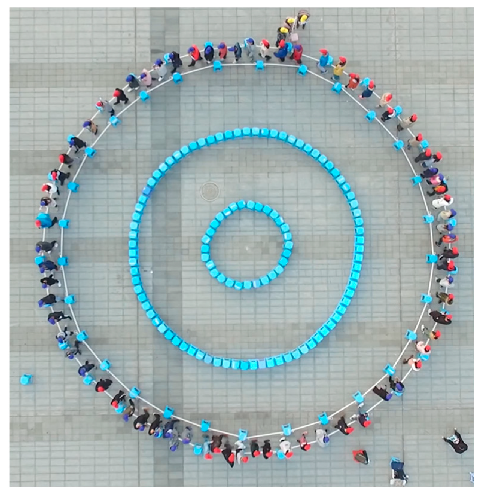
The basic configurations of this experiment can be seen in
Figure 1. (In
Figure 1, there is another ring road with a smaller radius and larger width. It is used for some other experiments, which is out of the scope of this paper. More details about these experiments can be found in Refs. [
20,
22]) The corridor width is 0.5 m, and the radius of this ring road is 8 m. In all the following simulations, the basic configurations of the ring road are exactly the same as that used in the previous experiments. Under periodic boundary conditions, the global density could be maintained, and the system was stable.
In the new model, in order to simulate single-file pedestrian flow at high densities, several modifications are considered:
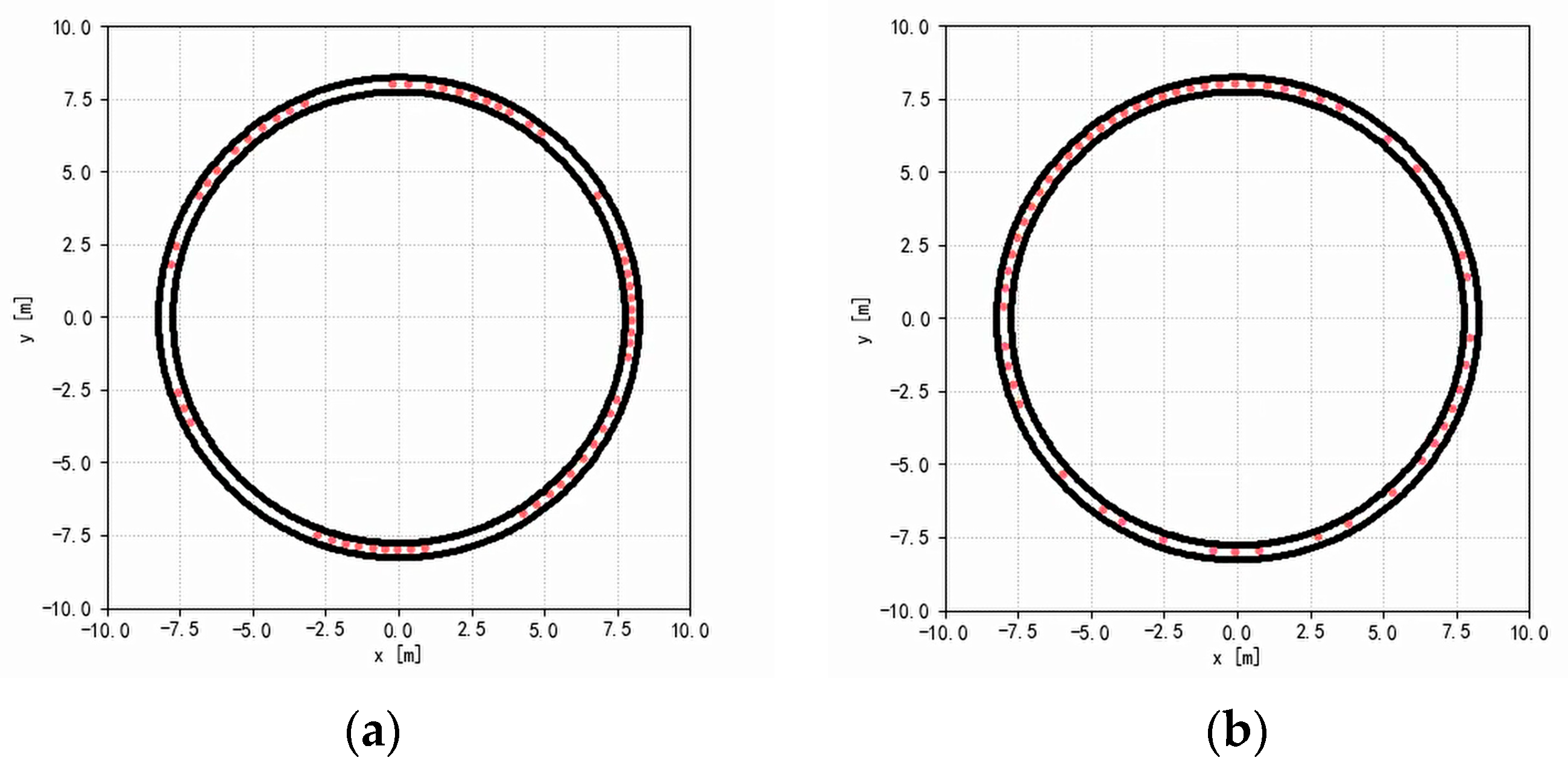
(1) The choice of the destination. In the single-file flow, usually the pedestrian needs to follow the preceding one, and he cannot overpass. For such a particular environment, if the traditional configuration in the original model is used, i.e., setting the destination of pedestrians as one fixed point, the simulation results may be not realistic. As shown in
Figure 2a, even when the density is low, the distribution of pedestrians may be strange. Some pedestrians are too close to the others, and there could be many spaces unused. Therefore, the new destination of a pedestrian is set as the current position of the preceding one in the simulations (If the two pedestrians are far from each other, the rule is still possible). By such a configuration, the problem could be solved in
Figure 2b; the distribution of pedestrians could be more reasonable at low densities, which is similar to that observed in the experiments [
20,
21].
(2) The distance for calculating forces between pedestrians. The critical distance is set as 0.8 m in the simulations. When the distance between the centers of pedestrians exceeds this threshold, the force is not considered. This approach makes the simulations faster, especially when the density is high.
(3) The configuration of obstacles. In the original model, the direction of the force is from the centroid of the ring road to the pedestrian’s position. However, this approach may lead to some problems, such as abnormal pedestrian trajectories. Sometimes, the pedestrians even leave the ring road. Therefore, in the new model, the obstacles (the two boundaries of the narrow corridor) are divided into N particles, with N set to 100 in this paper. Each particle can exert an influence on the nearby pedestrians from different angles, and the total forces are the combination of the N forces. Such a configuration effectively prevents pedestrians from leaving the road.
Furthermore, the means of determining the parameters in
Table 3 should be briefly introduced. It can be found that some parameters are significantly changed in the new model, including A
1, A
2, k
n1, k
n2, k
t1 and k
t2. Generally, if these parameters are not appropriate, there may be three unreasonable outcomes in the simulation, including:
(1) Repeated collision. For such a situation, the pedestrians may frequently collide with the two boundaries, and forward movement may be very difficult. This can also lead to lower averaged flow rates during the simulations.
(2) Inhomogeneous distribution. For such a situation, there are some large spaces on the ring road, and some pedestrians are too close to each other.
(3) Leaving the road. For such a situation, some pedestrians may be squeezed out of the ring road, which is apparently not reasonable.
All the above three situations are not observed in the single-file flow experiments. These phenomena indicate the parameters are either too large or too small, which produces abnormal forces on the pedestrians. For the simulations of single-file pedestrian flow, it is very difficult to use a unified optimization function to calibrate all the parameters. Therefore, the possible parameters are explored in
Table 4, and both the upper and lower limits of appropriate values are also given. The parameters within these ranges can lead to reasonable simulation results.
For a better understanding, some typical unreasonable simulation results are also shown in
Figure 3. For example, in
Figure 3a,c,f, some pedestrians are outside the ring road while, in
Figure 3b,d the distributions of pedestrians are quite inhomogeneous and many spaces are not effectively used. These bad situations further show the importance of appropriate parameters in the simulation of single-file pedestrian flow.
3. Simulation Results
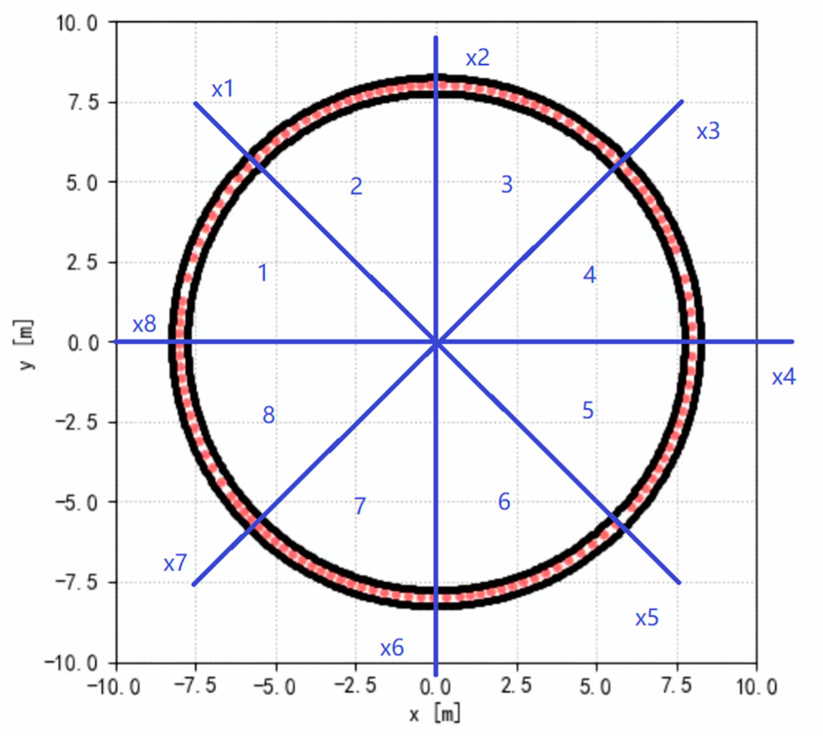
In this section, the simulation results produced by the modified social force model are discussed. Firstly, the fundamental diagrams are presented in
Figure 4. Here, the local maximum density as high as 4ped/m is reached. For the measurements of flows and densities, the ring road is divided into 8 equal subareas, as shown in
Figure 5. These subareas are named as 1, 2, …, 8, and the cross sections between them are named as x1, x2, …, x8. The local density is obtained by:
where N(t) is the pedestrian number in the subarea at time t;
is 15 s in the simulations (it is possible to consider other time intervals, but 15 s is good enough for the statistics in the experiments and simulations); and l
e is the length of one subarea, which is about 6.3 m.
The corresponding local flow rate
is obtained at the cross section between two subareas. At each location, the local flow rate is defined as:
where
is also 15 s and Q is the number of pedestrians who pass the cross section during the time interval (15 s).
The above measurements are exactly the same for both the experimental data and simulation results. It is clear that the simulation results quantitatively coincide with the experimental results, which is a good springboard for further studies.
Next, the simulated spatiotemporal diagrams will be discussed. Firstly, the results of the local flow rates are shown in
Figure 6. At low densities, the different regions with high flow rates and low flow rates alternatively emerge in
Figure 6a,b. Different colors could be clearly observed, which means that the distribution of pedestrians is not homogeneous at low densities. In fact, the speeds of all pedestrians are high at these low densities, as shown in the fundamental diagrams (
Figure 4). Thus, there is no congestion in
Figure 6a,b. In addition, some time–space diagrams, which correspond to
Figure 6, are shown in
Figure 7. Here, the orders of chosen pedestrians are No.1, No.5, No.9, …, etc. Since the simulation is performed on a ring road, the angular trajectories of pedestrians are presented, which is the same approach as that used for the experimental study. It was found that, although the speeds of all pedestrians are similar, the angular distances between these pedestrians are different in
Figure 7a,b, which also implies their spatial distribution is not homogeneous. This situation is qualitatively similar to that observed in the experiments.
When the densities become higher, the differences between the two types of regions gradually become not evident in
Figure 6c,d. This also means that the distribution of pedestrians become nearly homogeneous. Finally, when the density is very high in
Figure 6e,f, in most areas the flow rates are always very low, except one or two sections.
Furthermore, the results of local densities are shown in
Figure 8. When the densities are not high, the evolutions are qualitatively similar to that in
Figure 6; at low densities, the fluctuations are significant in
Figure 8a,b. At medium densities, the results become relatively homogeneous in
Figure 8c,d. However, at high densities, the situations are different. Especially in
Figure 8f, some areas (sections 5 and 6) are more congested than the others over a long time period. In fact, this phenomenon is also observed in the experiments [
21].
In the previous experimental study of single-file pedestrian flow [
21], some typical spatiotemporal diagrams at different densities have been shown. However, it is difficult to directly compare the appearances of the experimental and simulated spatiotemporal diagrams. Therefore, their statistical results can be compared, including the averaged values and standard deviations. Here, it is not necessary to show the averaged values of densities, since they are always constant on the ring road. On the contrary, the averaged values of flow rates at different densities can be studied. As shown in
Figure 9, it is clear that, in most subfigures, the averaged flow rates are nearly constant, which means the system is stable at all these densities. In addition, the two curves are quantitatively similar to each other, which further confirms the validity of the new model.
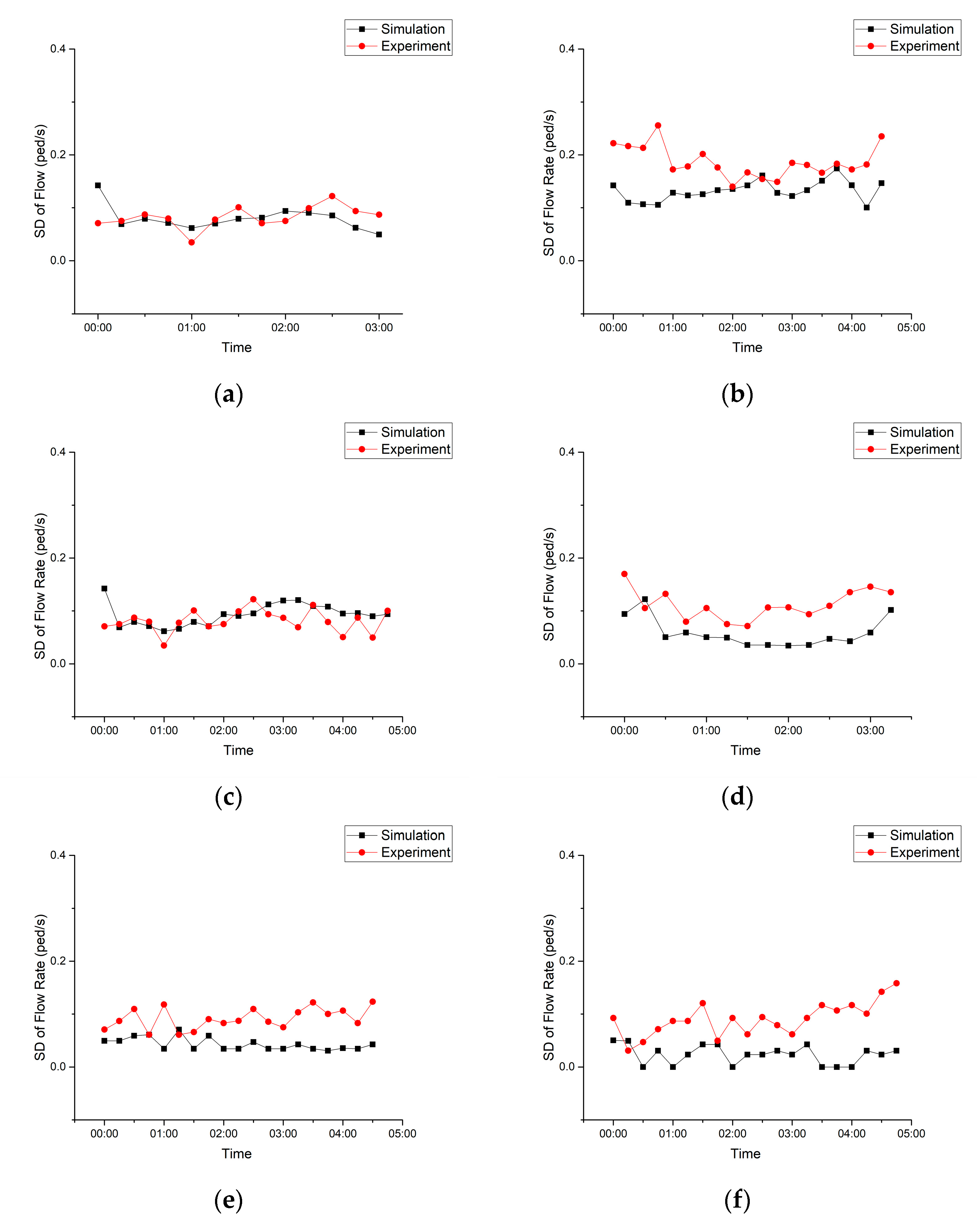
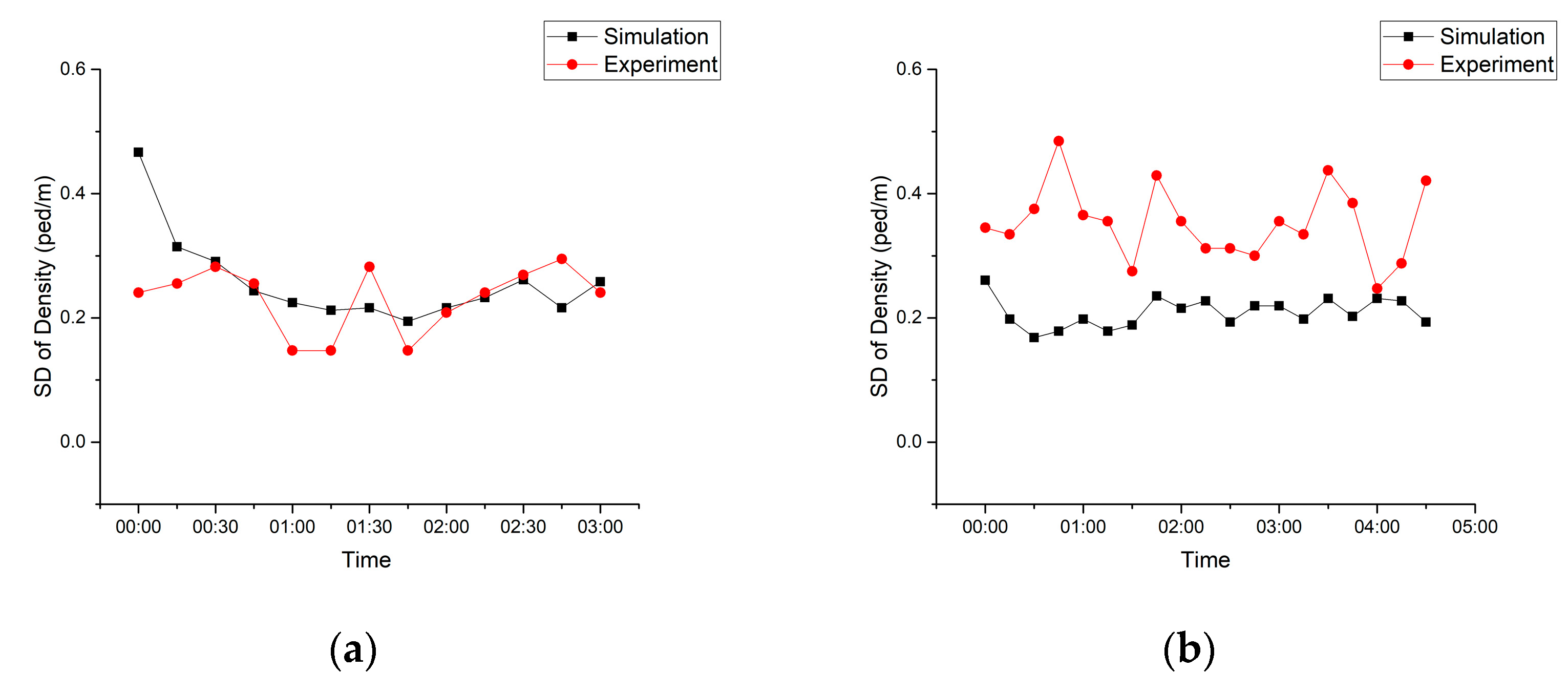
Additionally, the standard deviations of the flow rates are shown in
Figure 10, while those of the densities are presented in
Figure 11. Generally, the two curves in the many subfigures are close to each other, especially for the flow rates. However, it seems that, in some other figures, especially for densities, the results are a little different. For example, in
Figure 10, the simulation results are lower while, in
Figure 11e, the simulation results are higher. The tendencies in
Figure 11f are also different; the simulation results gradually decrease with time, while experimental results significantly fluctuate. The main reason could be that the simulation results in this paper are averaged ones, while the experimental results are just obtained from one run, which may not be typical for certain densities, and stochasticity cannot be ruled out. In the future, it is necessary to collect more data to verify these situations.
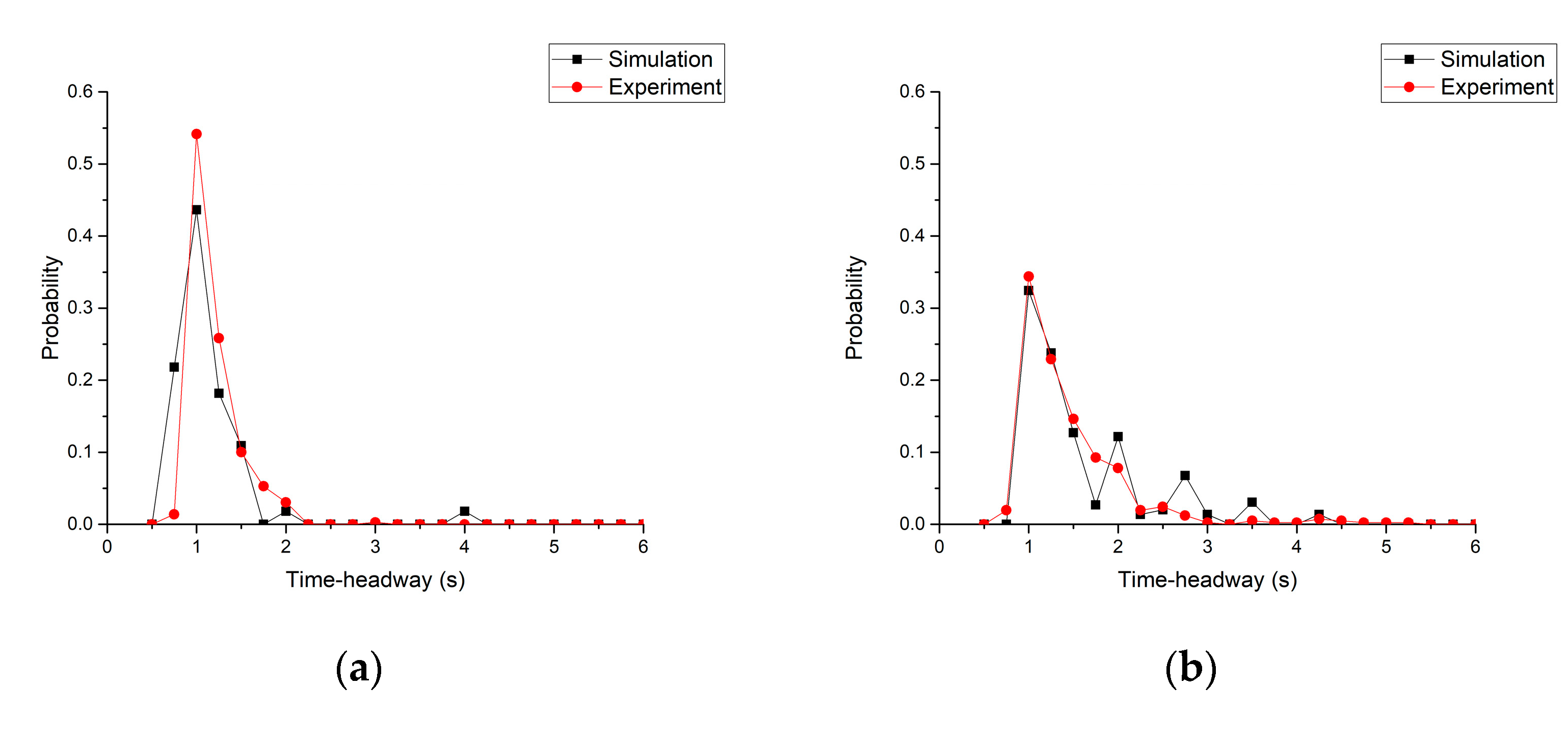
Excluding the macroscopic results discussed before, the microscopic analysis regarding the pedestrian movement is also important. Here, the time–headway distributions are chosen as examples, and the maximum value is set as 6s. As shown in
Figure 12, for all the densities the simulation results are similar to the experimental results; at low densities, there exists one evident peak in
Figure 12a,b. This is at about 1–2 s. However, with the increase in densities, the peak moves to the right side in
Figure 12c,d, and gradually disappears. Finally, the distribution becomes quite flat in
Figure 12e,f. In general, such tendencies are qualitatively similar to those observed in car-following behaviors, which also show some similarities between pedestrian flow and vehicular traffic flow.
4. Conclusions
In order to simulate single-file pedestrian movement, a new model is proposed based on the framework of Helbing’s social force model. Considering the phenomenon that the pedestrians can only follow the preceding one in the single-file flow, the way by which the pedestrian chooses their destination is changed. It is set as the current position of the preceding one, rather than at one fixed location in the corridor. Therefore, the desired force could be optimized. In addition, the distance for calculating forces between pedestrians is reset to 0.8 m, and the obstacles are divided into 100 particles. Furthermore, it was found that the original model parameters may lead to abnormal simulation results under high-density conditions. Therefore, the values of many parameters were reset. The possible ranges for reasonable results were also discussed. In the simulation results of the fundamental diagrams, spatiotemporal diagrams and the time–headway distributions, it can be found that the modified model can simulate single-file movement at high densities, even when the maximum local density is as high as 4ped/m. Comparisons between the statistical results at different global densities, including the averaged values and the standard deviations of local flow rates and local densities, show that, in most cases, the simulated and experimental results are quantitatively similar. The angular trajectories can help in understanding more about the simulation results. Some minor differences may result from the fact that the experimental dataset is not large enough. In short, this model could be a good choice for modeling single-file pedestrian flow at high densities.
Although lots of findings have been presented in this paper, there is much work to be carried out in the future. Firstly, in this paper, only the simple condition wherein there is no bottleneck is studied. If the bottleneck effect is involved, the experimental phenomena may be very complex [
17,
23], and whether the current model rules are suitable still needs to be investigated. Secondly, when there are more streams from different moving directions, the management of conflicts will be more challenging than the single-file flow, e.g., the counterflow [
24,
25,
26,
27,
28,
29,
30]. For such a task, perhaps the structure of social force models must be revised or extended due to these different environments. For example, in many countries, pedestrians prefer to move to the right side, which can help to form lanes in the counterflow. However, whether it could be helpful for the simulations by social force models is not clear. In addition, the individual characteristics of pedestrians (e.g., genders, body sizes or personality traits, etc.) are not considered in this paper, which could be explored in the future. In short, more data are needed, and there is still long way to go in this field.


