

A New Technique for Impervious Surface Mapping and Its Spatio-Temporal Changes from Landsat and Sentinel-2 Images

Abstract
:1. Introduction
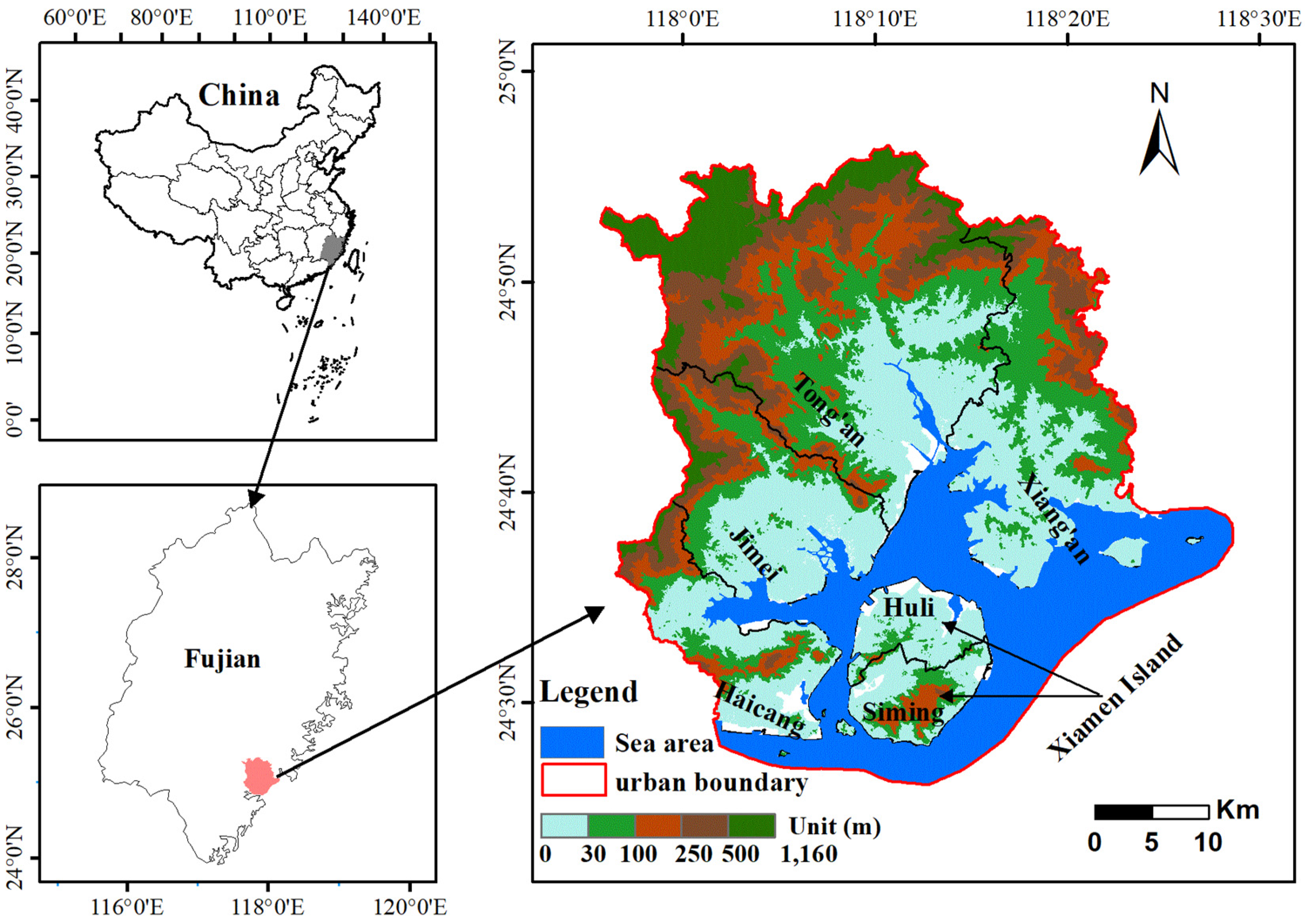
2. Study Area
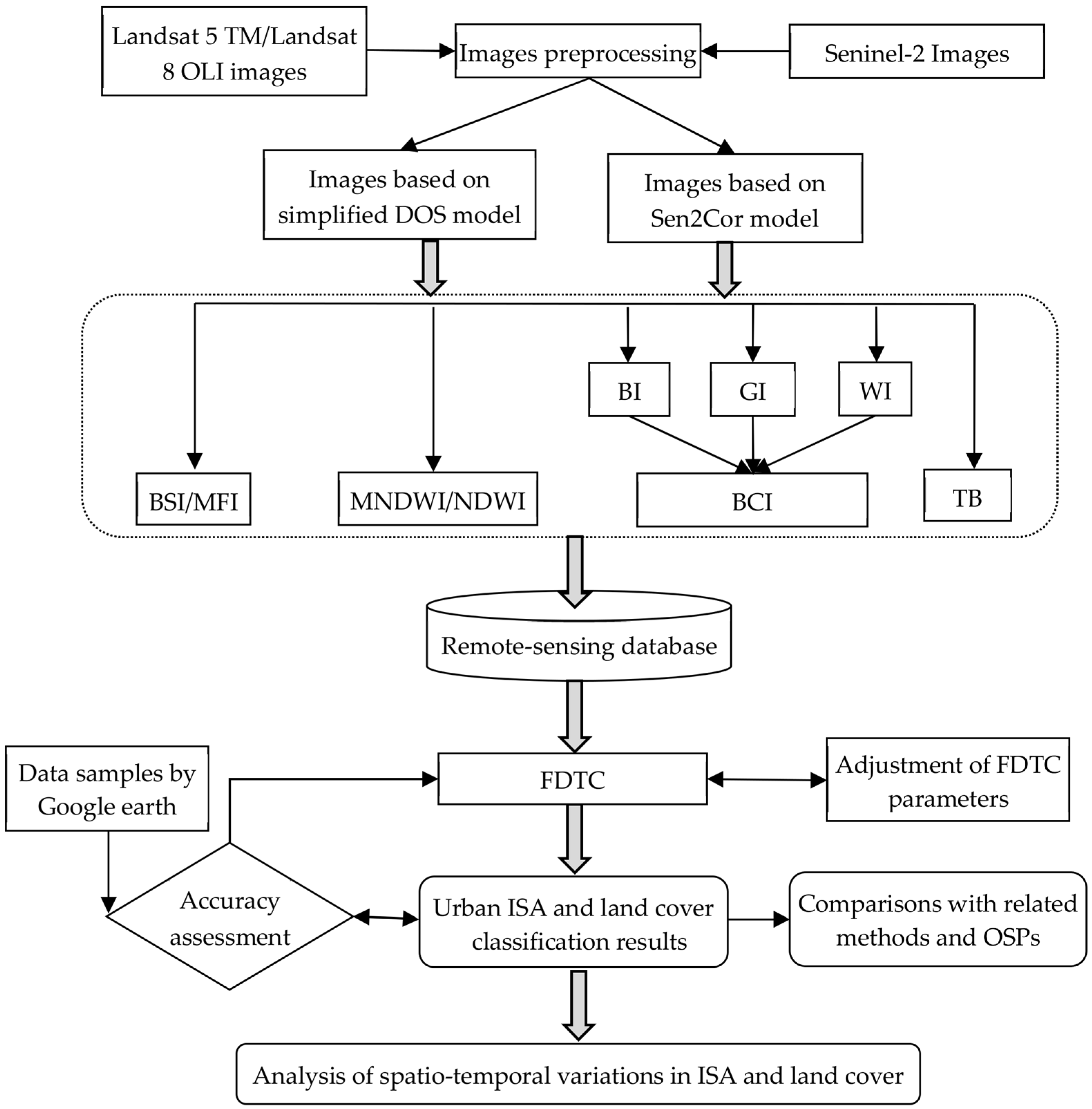
3. Materials and Methods
3.1. Data Collection and Preprocessing
3.2. Image-Based Atmospheric Correction Method
3.2.1. Simplified Top-of-the-Atmosphere Model
3.2.2. Simplified COST Model
3.2.3. Simplified DOS Model
3.2.4. Assessment of DOS and Sen2Cor
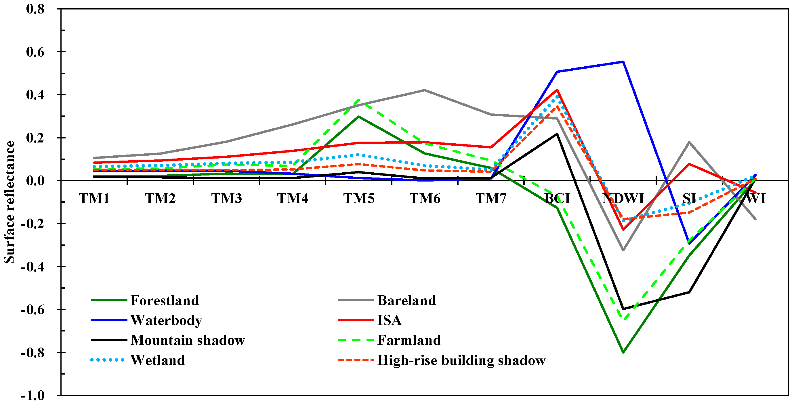
3.3. Feature Approach Based on Decision Tree Classification
3.3.1. Water Index
3.3.2. Bare Land Index
3.3.3. Impervious Index Based on Biophysical Composition Index
3.3.4. Brightness Temperature (TB)
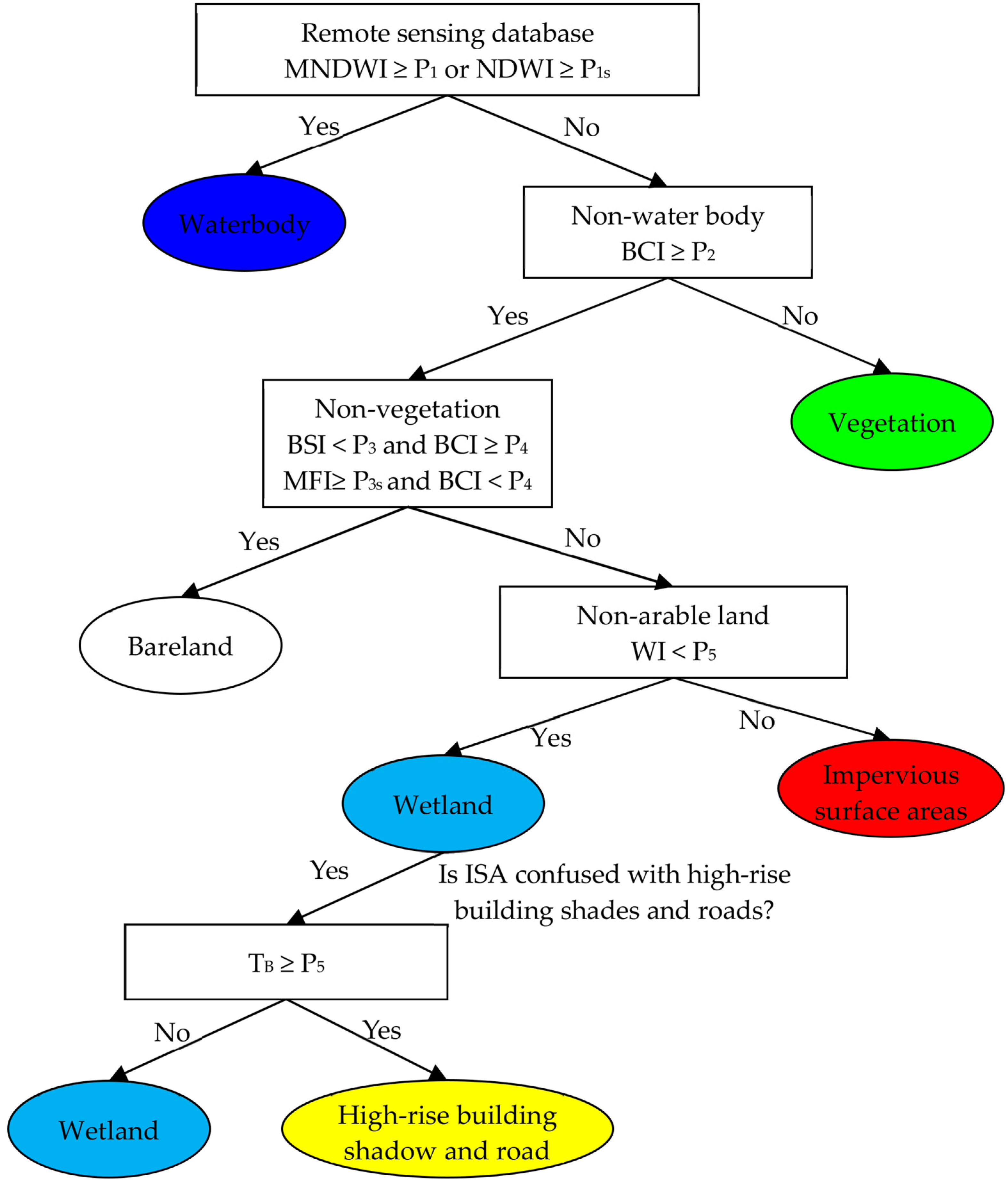
3.3.5. The Principle of FDTC
3.3.6. The Calibration of FDTC Parameters
3.4. Accuracy Assessment
4. Results and Discussion
4.1. Parameter Analysis for FDTC
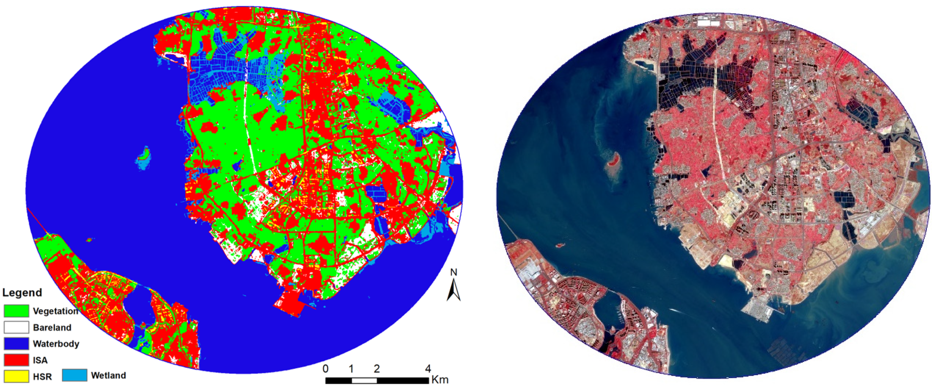
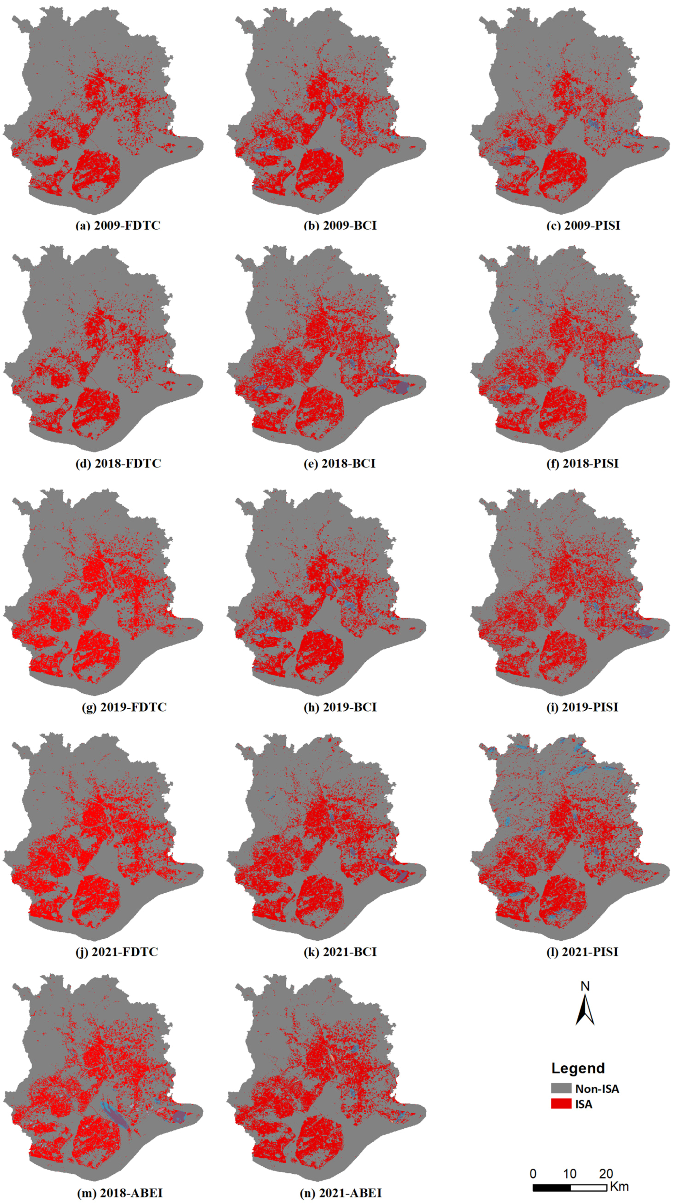
4.2. Analysis of Classification Accuracy for ISA
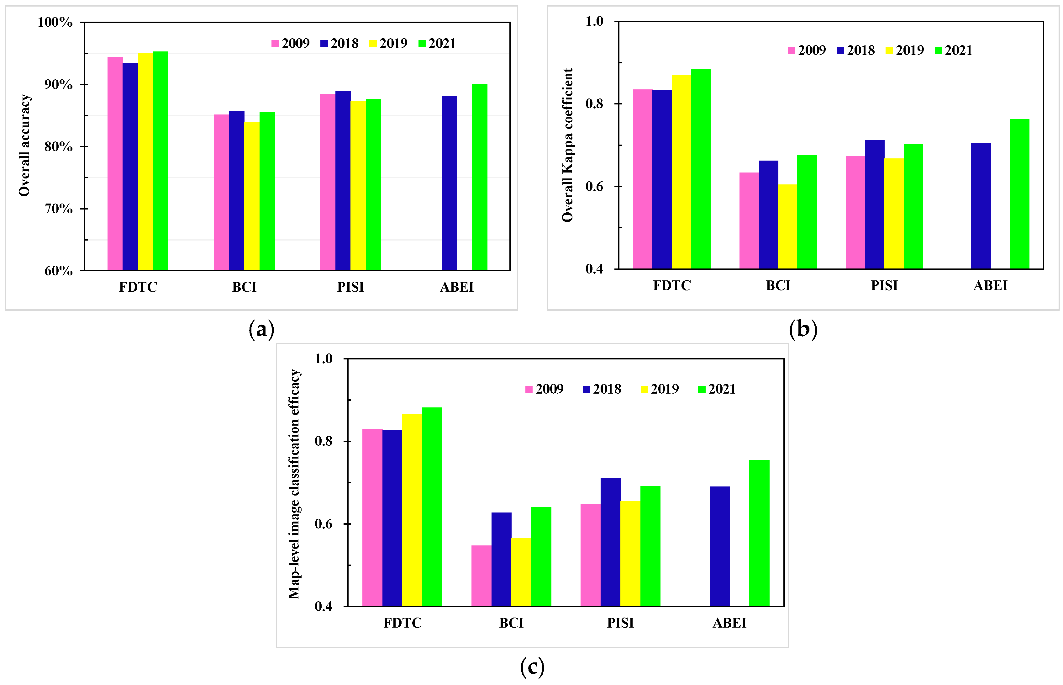
4.3. Comparison of ISA Classification Accuracy with Related Methods
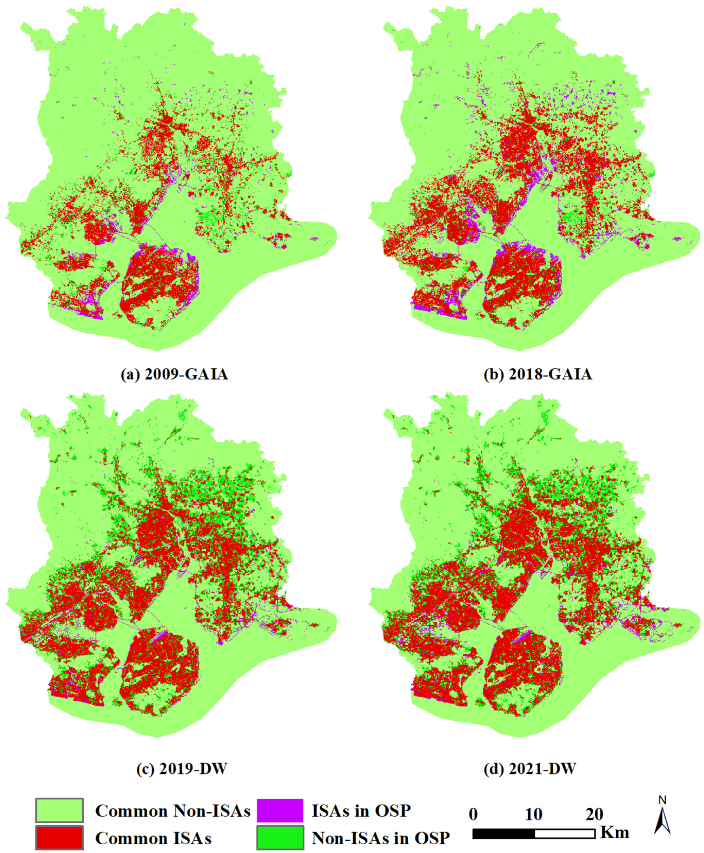
4.4. Comparison with Open-Source ISA Products
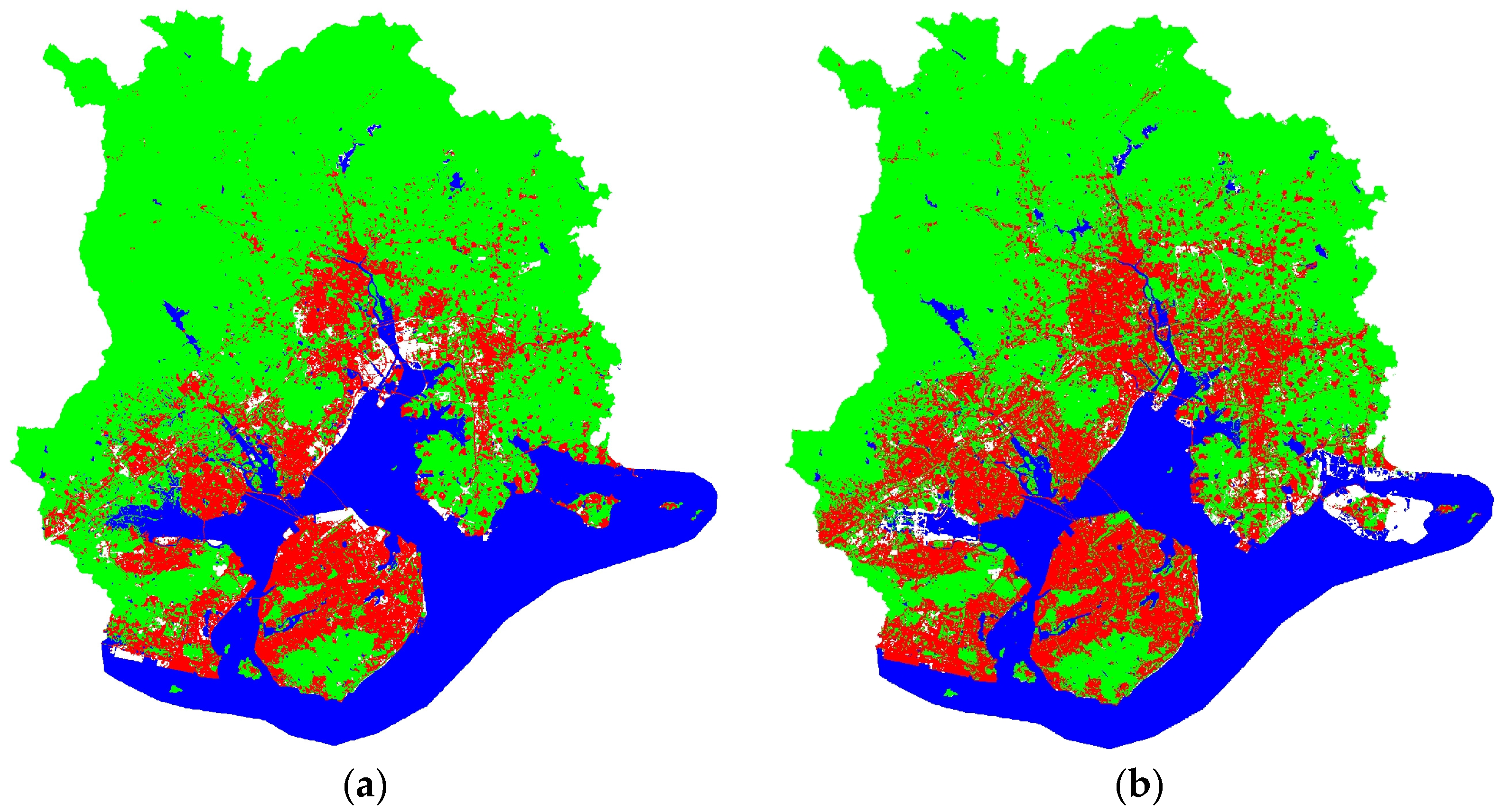
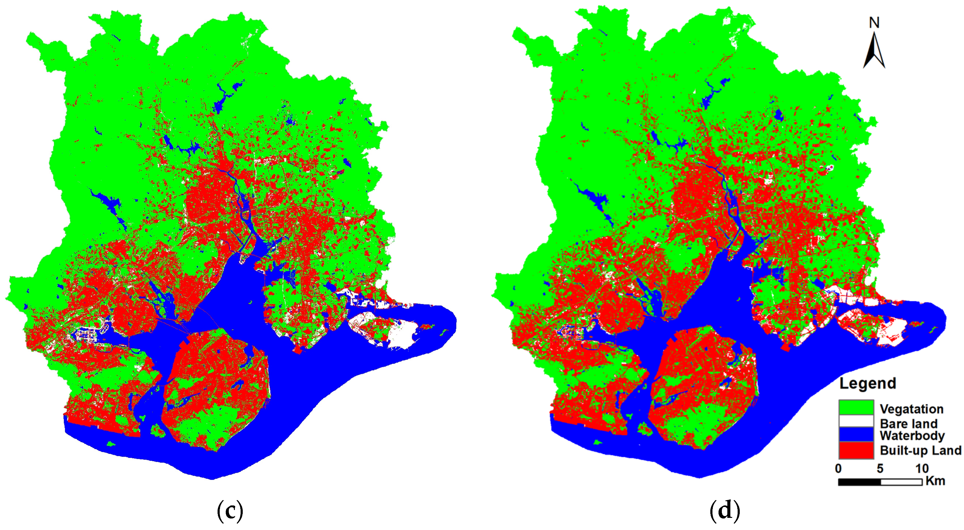
4.5. Analysis of Classification Accuracy for Land Cover
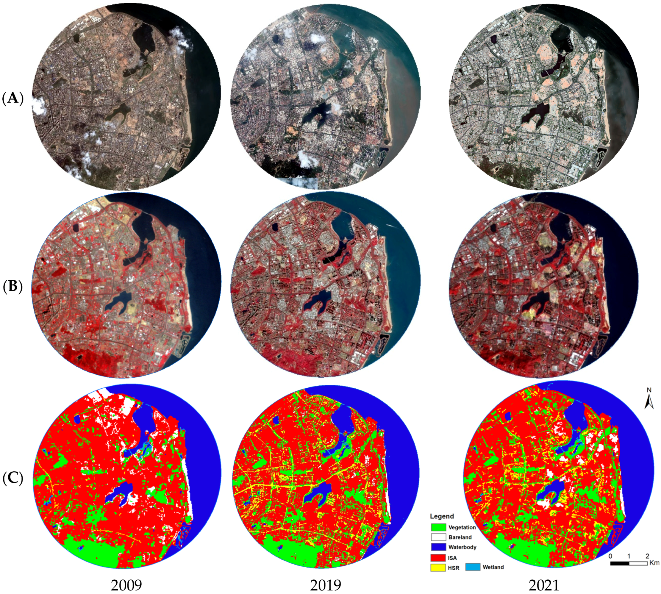
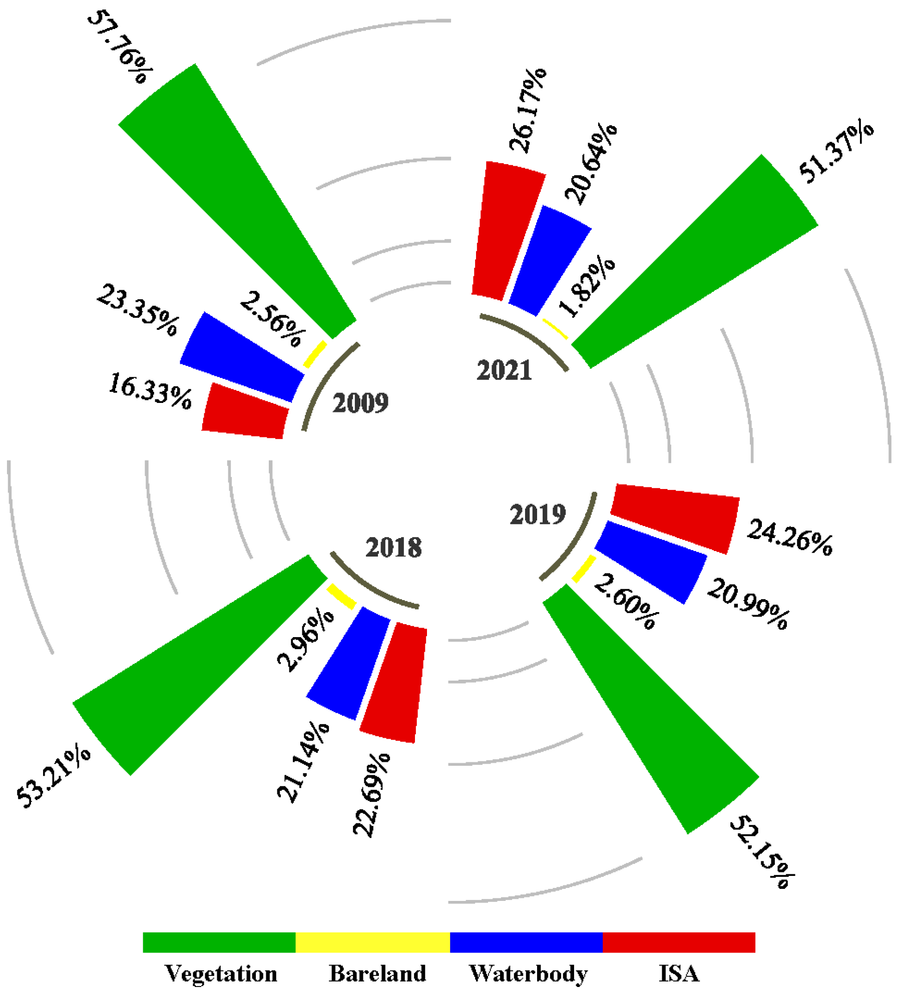
4.6. Spatiotemporal Land-Cover Changes
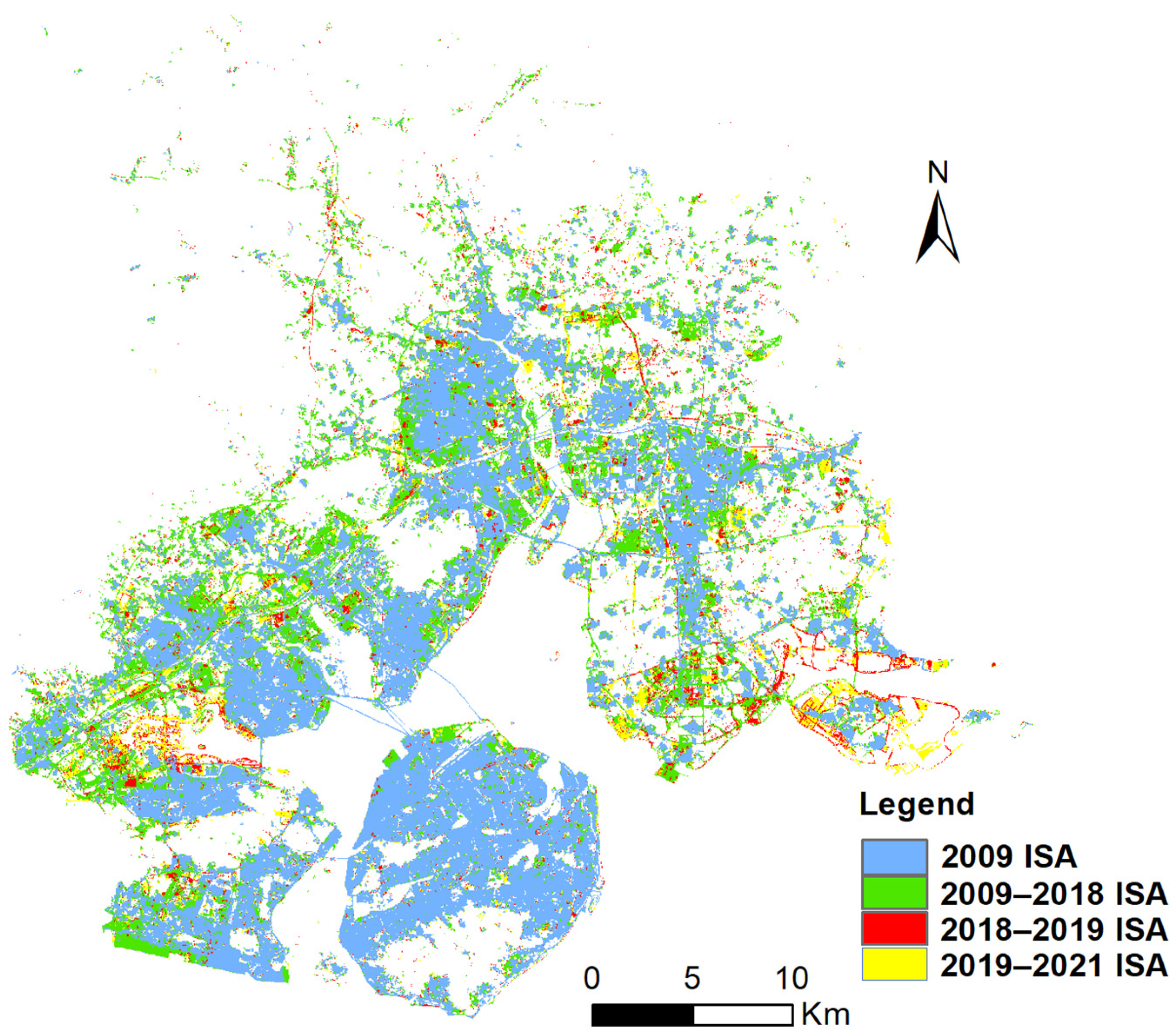
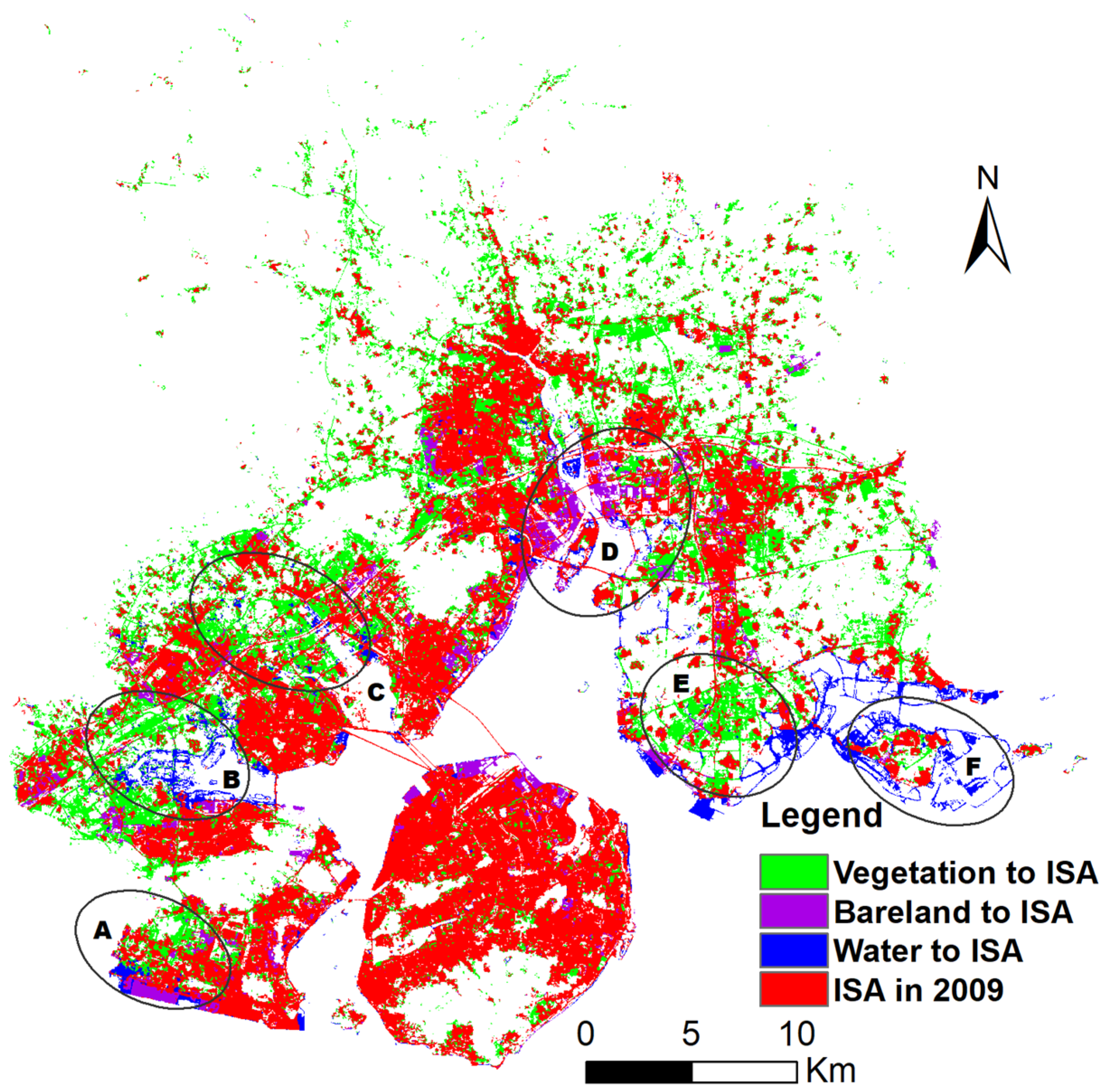
4.7. Spatiotemporal ISA Changes
5. Summary and Conclusions
Supplementary Materials
Author Contributions
Funding
Institutional Review Board Statement
Informed Consent Statement
Data Availability Statement
Conflicts of Interest
Abbreviations
| DTC | Decision tree classification |
| FDTC | Feature approach based on decision tree classification |
| ISAs | Impervious surface areas |
| NDWI | Normalized difference water index |
| MNDWI | Modified normalized difference water index |
| MFI | Mangrove forest index |
| BSI | Bare soil index |
| BCI | Biophysical composition index |
| GI | Greenness index |
| BI | Brightness index |
| WI | Wetness index |
| TB | Bright temperature |
| HSR | high-rise building shadows mixed with little roads |
| DN | Digital number |
| θ | Sun zenith angle |
| TOA | Top-of-the-atmosphere reflectance |
| DOS | Dark object subtraction |
| COST | A particular DOS approach calculating atmospheric transmittance using θ |
| TAUv | Atmospheric transmittance along the path from the earth’s surface to the sensor |
| TAUz | Atmospheric transmittance along the path from the sun to the earth’s surface |
| OA | Overall accuracy |
| KC | Overall kappa coefficient |
| MICE | Map-level image classification efficacy |
| AISA | Percent accuracy of ISA in common region between FDTC results and each ISA product |
| ANISA | Percent accuracy of non-ISA in common region between FDTC results and each ISA product |
| GE | Google Earth |
| PISI | Perpendicular impervious surface index |
| ABEI | Automated built-up extraction index |
| NDISI | Normalized difference impervious surface index |
| NBAI | Normalized built-up area index |
| BAEI | Built-up Area Extraction index |
| BUI | Built-up index |
| EBBI | Enhanced built-up and bareness index |
| BLFEI | Built-up land features extraction index |
| OB-NNC | Object-based nearest neighbor classification |
| OSPs | Open-source ISA products |
| GAIA | Global artificial impervious area |
| DW | Dynamic world |
References
- Kuang, W.; Zhang, S.; Li, X.; Lu, D. A 30 m resolution dataset of China’s urban impervious surface area and green space, 2000–2018. Earth. Syst. Sci. Data 2021, 13, 63–82. [Google Scholar] [CrossRef]
- Zhao, S.; Liu, S.; Zhou, D. Prevalent vegetation growth enhancement in urban environment. Proc. Natl. Acad. Sci. USA 2016, 113, 6313–6318. [Google Scholar] [CrossRef] [PubMed]
- Huang, F.; Yu, Y.; Feng, T. Automatic extraction of impervious surfaces from high resolution remote sensing images based on deep learning. J. Vis. Commun. Image Represent. 2019, 58, 453–461. [Google Scholar] [CrossRef]
- Tian, Y.; Chen, H.; Song, Q.; Zheng, K. A novel index for impervious surface area mapping: Development and validation. Remote Sens. 2018, 10, 1521. [Google Scholar] [CrossRef]
- Arnold, C.L., Jr.; Gibbons, C.J. Impervious surface coverage: The emergence of a key environmental indicator. J. Am. Plann. Assoc. 1996, 62, 243–258. [Google Scholar] [CrossRef]
- Ranagalage, M.; Estoque, R.C.; Murayama, Y. An Urban Heat Island Study of the Colombo Metropolitan Area, Sri Lanka, Based on Landsat Data (1997–2017). ISPRS Int. J. Geo-Inf. 2017, 6, 189. [Google Scholar] [CrossRef]
- Wang, M.; Xu, H. The impact of building height on urban thermal environment in summer: A case study of Chinese megacities. PLoS ONE 2021, 16, e0247786. [Google Scholar] [CrossRef]
- Arifwidodo, S.; Chandrasiri, O.; Abdulharis, R.; Kubota, T. Exploring the effects of urban heat island: A case study of two cities in Thailand and Indonesia. APN Sci. Bull. 2019, 9, 539. [Google Scholar] [CrossRef]
- Miller, J.D.; Hutchins, M. The impacts of urbanisation and climate change on urban flooding and urban water quality: A review of the evidence concerning the United Kingdom. J. Hydrol. Reg. Stud. 2017, 12, 345–362. [Google Scholar] [CrossRef]
- Zeiger, S.J.; Hubbart, J.A. Urban stormwater temperature surges: A central US watershed study. Hydrology 2015, 2, 193–209. [Google Scholar] [CrossRef]
- Santangelo, J.S.; Ness, R.W.; Cohan, B.; Fitzpatrick, C.R.; Innes, S.G.; Koch, S.; Lampei, C. Global urban environmental change drives adaptation in white clover. Science 2022, 375, 1275–1281. [Google Scholar] [CrossRef] [PubMed]
- Weng, Q. Remote sensing of impervious surfaces in the urban areas: Requirements, methods, and trends. Remote Sens. Environ. 2012, 117, 34–49. [Google Scholar] [CrossRef]
- Deng, H.; Liu, T.; Zhao, J. Strategic measures for an integrated approach to sustainable development in Lijiang City. Int. J. Sust. Dev. World 2011, 18, 559–562. [Google Scholar] [CrossRef]
- Hua, L.; Zhang, X.; Nie, Q.; Sun, F.; Tang, L. The impacts of the expansion of urban impervious surfaces on urban heat islands in a coastal city in China. Sustainability 2020, 12, 475. [Google Scholar] [CrossRef]
- Pal, M.; Mather, P.M. An assessment of the effectiveness of decision tree methods for land cover classification. Remote Sens. Environ. 2003, 86, 554–565. [Google Scholar] [CrossRef]
- Xian, G.; Crane, M. An analysis of urban thermal characteristics and associated land cover in tampa bay and Las Vegas using Landsat satellite data. Remote Sens. Environ. 2006, 104, 147–156. [Google Scholar] [CrossRef]
- Hu, B.; Xu, Y.; Huang, X.; Cheng, Q.; Ding, Q.; Bai, L.; Li, Y. Improving Urban Land Cover Classification with Combined Use of Sentinel-2 and Sentinel-1 Imagery. ISPRS Int. J. Geo-Inf. 2021, 10, 533. [Google Scholar] [CrossRef]
- Voorde, T.V.D.; Roeck, T.D.; Canters, F. A comparison of two spectral mixture modelling approaches for impervious surface mapping in urban areas. Int. J. Remote Sens. 2009, 30, 4785–4806. [Google Scholar] [CrossRef]
- Han, Y.; Liu, Y.; Hong, Z.; Zhang, Y.; Yang, S.; Wang, J. Sea ice image classification based on heterogeneous data fusion and deep learning. Remote Sens. 2021, 13, 592. [Google Scholar] [CrossRef]
- Junaid, M.; Sun, J.; Iqbal, A.; Sohail, M.; Zafar, S.; Khan, A. Mapping LULC Dynamics and Its Potential Implication on Forest Cover in Malam Jabba Region with Landsat Time Series Imagery and Random Forest Classification. Sustainability 2023, 15, 1858. [Google Scholar] [CrossRef]
- Li, J.; Song, C.; Cao, L.; Zhu, F.G.; Meng, X.L.; Wu, J.G. Impacts of landscape structure on surface urban heat islands: A case study of Shanghai, China. Remote Sens. Environ. 2011, 115, 3249–3263. [Google Scholar] [CrossRef]
- Powell, R.L.; Roberts, D.A.; Dennison, P.E.; Hess, L.L. Sub-pixel mapping of urban land cover using multiple endmember spectral mixture analysis: Manaus, Brazil. Remote Sens. Environ. 2007, 106, 253–267. [Google Scholar] [CrossRef]
- Zha, Y.; Gao, J.; Ni, S. Use of normalized difference built-up index in automatically mapping urban areas from TM imagery. Int. J. Remote Sens. 2003, 24, 583–594. [Google Scholar] [CrossRef]
- Xu, H. A new index for delineating built-up land features in satellite imagery. Int. J. Remote Sens. 2008, 29, 4269–4276. [Google Scholar] [CrossRef]
- Kawamura, M.; Jayamana, S.; Tsujiko, Y. Relation between social and environmental conditions in Colombo srilanka and the urban index estimated by satellite remote sensing data. Int. Soc. Photogramm. Remote Sens. 1996, 31, 321–326. [Google Scholar]
- Deng, C.; Wu, C. BCI: A biophysical composition index for remote sensing of urban environments. Remote Sens. Environ. 2012, 127, 247–259. [Google Scholar] [CrossRef]
- Sun, G.; Chen, X.; Jia, X.; Yao, Y.; Wang, Z. Combinational build-up index (CBI) for effective impervious surface mapping in urban areas. IEEE J. Sel. Top. Appl. Earth Obs. Remote Sens. 2017, 9, 2081–2092. [Google Scholar] [CrossRef]
- Firozjaei, M.K.; Sedighi, A.; Kiavarz, M.; Qureshi, S.; Haase, D.; Alavipanah, S.K. Automated built-up extraction index: A new technique for mapping surface built-up areas using Landsat 8 OLI imagery. Remote Sens. 2019, 11, 1966. [Google Scholar] [CrossRef]
- Xu, H. Analysis of impervious surface and its impact on urban heat environment using the normalized difference impervious surface index (NDISI). Photogramm. Eng. Remote Sens. 2010, 76, 557–565. [Google Scholar] [CrossRef]
- Waqar, M.M.; Mirza, J.F.; Mumtaz, R.; Hussain, E. Development of new indices for extraction of built-up area & bare soil from landsat data. Open Access Sci. Rep. 2012, 1, 136. [Google Scholar]
- Bouzekri, S.; Lasbet, A.A.; Lachehab, A. A new spectral index for extraction of built-up area using landsat-8 data. J. Indian Soc. Remote Sens. 2015, 43, 867–873. [Google Scholar] [CrossRef]
- As-Syakur, A.R.; Adnyana, I.W.S.; Arthana, I.W.; Nuarsa, I.W. Enhanced built-up and bareness index (EBBI) for mapping built-up and bare land in an urban area. Remote Sens. 2012, 4, 2957–2970. [Google Scholar] [CrossRef]
- Kaimaris, D.; Patias, P. Identification and area measurement of the built-up area with the Built-up Index (BUI). Int. J. Adv. Remote Sens. GIS 2016, 5, 1844–1858. [Google Scholar] [CrossRef]
- Bouhennache, R.; Bouden, T.; Taleb-Ahmed, A.; Cheddad, A. A new spectral index for the extraction of built-up land features from Landsat 8 satellite imagery. Geocarto Int. 2019, 34, 1531–1551. [Google Scholar] [CrossRef]
- Lu, D.; Mausel, P. Assessment of atmospheric correction methods for Landsat TM data applicable to Amazon basin LBA research. Int. J. Remote Sens. 2002, 23, 2651–2671. [Google Scholar] [CrossRef]
- Martins, V.S.; Barbosa, C.C.F.; De Carvalho, L.A.S.; Jorge, D.S.F.; Lobo, F.D.L.; Novo, E.M.L.D.M. Assessment of atmospheric correction methods for Sentinel-2 MSI images applied to Amazon floodplain lakes. Remote Sens. 2017, 9, 322. [Google Scholar] [CrossRef]
- Kebede, T.A.; Hailu, B.T.; Suryabhagavan, K.V. Evaluation of spectral built-up indices for impervious surface extraction using Sentinel-2A MSI imageries: A case of Addis Ababa city, Ethiopia. Environ. Chall. 2022, 8, 100568. [Google Scholar] [CrossRef]
- Deliry, S.I.; Avdan, Z.Y.; Avdan, U. Extracting urban impervious surfaces from Sentinel-2 and Landsat-8 satellite data for urban planning and environmental management. Environ. Sci. Pollut. Res. 2021, 28, 6572–6586. [Google Scholar] [CrossRef]
- Tian, Y.; Yin, K.; Lu, D.; Hua, L.; Zhao, Q.; Wen, M. Examining land use and land cover spatiotemporal change and driving forces in beijing from 1978 to 2010. Remote Sens. 2014, 6, 10593–10611. [Google Scholar] [CrossRef]
- Tang, L.N.; Zhao, Y.; Yin, K.; Zhao, J. City profile: Xiamen. Cities 2013, 31, 615–624. [Google Scholar] [CrossRef]
- Hua, L.Z.; Li, X.Q.; Tang, L.N.; Yin, K.; Zhao, Y. Spatio-temporal dynamic analysis of island-city landscape: A case study of Xiamen Island, China. Int. J. Sust. Dev. World 2010, 17, 273–278. [Google Scholar] [CrossRef]
- Sola, I.; García-Martín, A.; Sandonís-Pozo, L.; Álvarez-Mozos, J.; Pérez-Cabello, F.; González-Audícana, M.; Llovería, R.M. Assessment of atmospheric correction methods for Sentinel-2 images in Mediterranean landscapes. Int. J. Appl. Earth. Obs. 2018, 73, 63–76. [Google Scholar] [CrossRef]
- Chander, G.; Markham, B.L.; Helder, D.L. Summary of current radiometric calibration coefficients for Landsat MSS, TM, ETM+, and EO-1 ALI sensors. Remote Sens. Environ. 2009, 113, 893–903. [Google Scholar] [CrossRef]
- Chavez, P.S. Image-based atmospheric corrections-revisited and improved. Photogramm. Eng. Remote Sens. 1996, 62, 1025–1036. [Google Scholar]
- Ramsey, R.D.; Wright, D.L.; Mcginty, C. Evaluating the use of Landsat 30m enhanced thematic mapper to monitor vegetation cover in shrub-steppe environments. Geocarto Int. 2004, 19, 39–47. [Google Scholar] [CrossRef]
- Xu, H. Retrieval of the reflectance and land surface temperature of the newly-launched Landsat 8 satellite. Chin. J. Geophys. 2015, 58, 741–747. (In Chinese) [Google Scholar]
- Yang, X.; Lo, C.P. Relative radiometric normalization performance for change detection from multi-date satellite images. Photogramm. Eng. Remote Sens. 2000, 66, 967–980. [Google Scholar]
- Friedl, M.A.; Brodleyf, C.E. Decision tree classification of land cover from remotely sensed data. Remote Sens. Environ. 1997, 61, 399–409. [Google Scholar] [CrossRef]
- Punia, M.; Joshi, P.K.; Porwal, M.C. Decision tree classification of land use land cover for Delhi, India using IRS-P6 AWiFS data. Expert Syst. Appl. 2011, 38, 5577–5583. [Google Scholar] [CrossRef]
- Qi, Z.; Yeh, A.G.O.; Li, X.; Lin, Z. A novel algorithm for land use and land cover classification usingRADARSAT-2 polarimetric SAR data. Remote Sens. Environ. 2012, 118, 21–39. [Google Scholar] [CrossRef]
- McFeeters, S.K. The use of the Normalized Difference Water Index (NDWI) in the delineation of open water features. Int. J. Remote Sens. 1996, 17, 1425–1432. [Google Scholar] [CrossRef]
- Xu, H. Modification of normalised difference water index (NDWI) to enhance open water features in remotely sensed imagery. Int. J. Remote Sens. 2006, 27, 3025–3033. [Google Scholar] [CrossRef]
- Xu, H.; Wang, M.; Shi, T.; Guan, H.; Fang, C.; Lin, Z. Prediction of ecological effects of potential population and impervious surface increases using a remote sensing based ecological index (RSEI). Ecol. Indic. 2018, 93, 730–740. [Google Scholar] [CrossRef]
- Rikimaru, A.; Roy, P.S.; Miyatake, S. Tropical Forest cover density mapping. Trop. Ecol. 2002, 43, 39–47. [Google Scholar]
- Jia, M.; Wang, Z.; Wang, C.; Mao, D.; Zhang, Y. A new vegetation index to detect periodically submerged mangrove forest using single-tide sentinel-2 imagery. Remote Sens. 2019, 11, 2043. [Google Scholar] [CrossRef]
- Crist, E.P. A TM tasseled cap equivalent transformation for reflectance factor data. Remote Sens. Environ. 1985, 17, 301–306. [Google Scholar] [CrossRef]
- Baig, M.H.; Zhang, L.; Shuai, T.; Tong, Q. Derivation of a tasselled cap transformation based on Landsat 8 at-satellite reflectance. Remote Sens. Lett. 2014, 5, 423–431. [Google Scholar] [CrossRef]
- Shi, T.; Xu, H. Derivation of Tasseled Cap Transformation coefficients for Sentinel-2 MSI at-sensor reflectance data. IEEE J.-Stars. 2019, 12, 4038–4048. [Google Scholar] [CrossRef]
- Li, F.; Jackson, T.J.; Kustas, W.P.; Schmugge, T.J.; French, A.N.; Cosh, M.H.; Bindlish, R. Deriving land surface temperature from Landsat 5 and 7 during SMEX02/SMACEX. Remote Sens. Environ. 2004, 92, 521–534. [Google Scholar] [CrossRef]
- Congalton, R.G. A review of assessing the accuracy of classifications of remotely sensed data. Remote Sens. Environ. 1991, 37, 35–46. [Google Scholar] [CrossRef]
- Landis, J.R.; Koch, G.G. The measurement of observer agreement for categorical data. Biometrics 1977, 33, 159–174. [Google Scholar] [CrossRef]
- Shao, G.; Tang, L.; Liao, J. Overselling overall map accuracy misinforms about research reliability. Landsc. Ecol. 2019, 34, 2487–2492. [Google Scholar] [CrossRef]
- Shao, G.; Tang, L.; Zhang, H. Introducing image classification efficacies. IEEE Access 2021, 9, 134809–134816. [Google Scholar] [CrossRef]
- Gong, P.; Li, X.; Wang, J.; Bai, Y.; Chen, B.; Hu, T.; Zhou, Y. Annual maps of global artificial impervious area (GAIA) between 1985 and 2018. Remote Sens. Environ. 2020, 236, 111510. [Google Scholar] [CrossRef]
- Brown, C.F.; Brumby, S.P.; Guzder-Williams, B.; Birch, T.; Hyde, S.B.; Mazzariello, J.; Tait, A.M. Dynamic World, Near real-time global 10 m land use land cover mapping. Sci. Data 2022, 9, 251. [Google Scholar] [CrossRef]
- Chen, Y.; Zhang, G.; Cui, H.; Li, X.; Hou, S.; Ma, J.; Li, Z.; Li, H.; Wang, H. A novel weakly supervised semantic segmentation framework to improve the resolution of land cover product. ISPRS Photogramm. Eng. Remote Sens. 2023, 196, 73–92. [Google Scholar] [CrossRef]
- Lin, T.; Xue, X.; Shi, L.; Gao, L. Urban spatial expansion and its impacts on island ecosystem services and landscape pattern: A case study of the island city of Xiamen, Southeast China. Ocean Coast. Manag. 2013, 81, 90–96. [Google Scholar] [CrossRef]
- Zhang, L.; Yang, L.; Zohner, C.M.; Crowther, T.W.; Li, M.; Shen, F.; Zhou, C. Direct and indirect impacts of urbanization on vegetation growth across the world’s cities. Sci. Adv. 2022, 8, eabo0095. [Google Scholar] [CrossRef] [PubMed]


| Date | Image Sensor | Sun Azimuth Angle | Sun-Elevation Angle | WRS Path-Row/ Orbit-Tile Number |
|---|---|---|---|---|
| 6 June 2009 | Landsat 5 TM | 89.28 | 66.34 | 119-043 |
| 11 March 2018 | Landsat 8 OLI/TIRS | 134.98 | 52.19 | 119-043 |
| 15 November 2019 | Sentinel-2 | 159.05 | 42.80 | 89-T50RPN |
| 15 November 2019 | Sentinel-2 | 157.75 | 43.14 | 89-T50RNN |
| 16 December 2021 | Landsat 8 OLI/TIRS | 154.33 | 37.61 | 119-043 |
| Name | Landsat 8/Landsat 5 | Remark |
|---|---|---|
| TOA | ||
| DOS | ||
| COST |
| Sensor Type | Year | MNDWI/ (P1) | NDWI (P1s) | BCI (P2) | BSI and BCI (P3 and P4) | MFI and BCI (P3s and P4) | WI (P5) | TB(P6) |
|---|---|---|---|---|---|---|---|---|
| Landsat-5 | 2009 | −0.05 | / | 0.13 | 0.17 and 0.75 | / | −0.10 | 301.00 |
| Landsat-8 | 2018 | 0 | / | 0.06 | 0.15 and 0.4 | / | −0.04 | 292.86 |
| Sentinel-2 | 2019 | / | 0.09 | 0.05 | 0.25 and 0.4 | −0.15 | 299.70 | |
| Landsat-8 | 2021 | / | 0.02 | 0.14 | 0.13 and 0.4 | 0 | 299.80 |
| Authors | Methods | Sensors | OA% | KC |
|---|---|---|---|---|
| Tian et al. [4] | PISI | Landsat 8 | 89.51~96.50 | 0.79~0.93 |
| Xu [29] | NDISI | Landsat ETM+ | 90.70 | 0.81 |
| Firozjaei et al. [28] | ABEI | Landsat 8 | 92.04~97.62 | 0.90~0.96 |
| As-syakur et al. [32] | EBBI | Landsat ETM+ | 88.98 | / |
| Kaimaris et al. [33] | BUI | Landsat ETM+ | 90 | 0.8 |
| Waqar et al. [30] | NBAI | Landsat 5 TM | 86.87 | 0.73 |
| Kebede et al. [37] | NBAI | Sentinel-2 | 93~97 | 0.86~0.92 |
| Bouhennache et al. [34] | BLFEI | Landsat 8 | 95 | 0.9 |
| Bouzekri et al. [31] | BAEI | Landsat 8 | 92.66 | 0.85 |
| Deliry et al. [38] | OB-NNC | Sentinel-2 Landsat 8 | 90.91 88.64 | 0.82 0.77 |
| Hua et al. (this study) | FDTC | Landsat 5 TM | 94.40 | 0.84 |
| Landsat 8 | 93.41~95.27 | 0.83~0.89 | ||
| Sentinel-2 | 95.05 | 0.87 |
| Year | ISA Product Type | AISA (%) | ANISA (%) |
|---|---|---|---|
| 2009 | GAIA | 73.25 | 98.54 |
| 2018 | GAIA | 80.47 | 96.81 |
| 2019 | DW | 91.91 | 82.89 |
| 2021 | DW | 99.37 | 83.41 |
| Average | 86.25 | 90.41 |
| Sensors | Date | OA (%) | KC | MICE |
|---|---|---|---|---|
| Landsat 5 TM | June 2009 | 91.10 | 0.869 | 0.869 |
| Landsat 8 OLI | March 2018 | 90.77 | 0.865 | 0.865 |
| Sentinel-2 | November 2019 | 91.54 | 0.879 | 0.879 |
| Landsat 8 OLI | December 2021 | 92.74 | 0.895 | 0.895 |
Disclaimer/Publisher’s Note: The statements, opinions and data contained in all publications are solely those of the individual author(s) and contributor(s) and not of MDPI and/or the editor(s). MDPI and/or the editor(s) disclaim responsibility for any injury to people or property resulting from any ideas, methods, instructions or products referred to in the content. |
© 2023 by the authors. Licensee MDPI, Basel, Switzerland. This article is an open access article distributed under the terms and conditions of the Creative Commons Attribution (CC BY) license (https://creativecommons.org/licenses/by/4.0/).
Share and Cite
Hua, L.; Wang, H.; Zhang, H.; Sun, F.; Li, L.; Tang, L. A New Technique for Impervious Surface Mapping and Its Spatio-Temporal Changes from Landsat and Sentinel-2 Images. Sustainability 2023, 15, 7947. https://doi.org/10.3390/su15107947
Hua L, Wang H, Zhang H, Sun F, Li L, Tang L. A New Technique for Impervious Surface Mapping and Its Spatio-Temporal Changes from Landsat and Sentinel-2 Images. Sustainability. 2023; 15(10):7947. https://doi.org/10.3390/su15107947
Chicago/Turabian StyleHua, Lizhong, Haibo Wang, Huafeng Zhang, Fengqin Sun, Lanhui Li, and Lina Tang. 2023. "A New Technique for Impervious Surface Mapping and Its Spatio-Temporal Changes from Landsat and Sentinel-2 Images" Sustainability 15, no. 10: 7947. https://doi.org/10.3390/su15107947