Article

Nonlinear Relationships between Vehicle Ownership and Household Travel Characteristics and Built Environment Attributes in the US Using the XGBT Algorithm

1
School of Tourism, Dalian University, Dalian 116000, China
2
Centre for Sustainable Urban Planning and Real Estate (SUPRE), Department of Urban and Regional Planning, Faculty of Built Environment, University of Malaya, Kuala Lumpur 50603, Malaysia
3
Department of Civil and Environmental Engineering, Universiti Teknologi PETRONAS, Seri Iskandar 32610, Malaysia
4
Faculty of Hospitality, Tourism and Wellness. Universiti Malaysia Kelantan, City Campus, Pengkalan Chepa 16100, Malaysia
5
Department of Civil Engineering, College of Engineering, Prince Sattam Bin Abdulaziz University, Alkharj 16273, Saudi Arabia
6
Building & Construction Technology Department, Bayan College of Science and Technology, Khartoum 210, Sudan
7
Research Centre, Future University in Egypt, New Cairo 11745, Egypt
*
Authors to whom correspondence should be addressed.
Sustainability 2022, 14(6), 3395; https://doi.org/10.3390/su14063395
Submission received: 4 February 2022 / Revised: 1 March 2022 / Accepted: 4 March 2022 / Published: 14 March 2022
(This article belongs to the Collection Urban Street Networks and Sustainable Transportation)

Abstract

:
In the United States, several studies have looked at the association between automobile ownership and sociodemographic factors and built environment qualities, but few have looked at household travel characteristics. Their interactions and nonlinear linkages are frequently overlooked in existing studies. Utilizing the 2017 US National Household Travel Survey, the authors employed an extreme gradient boosting tree model to evaluate the nonlinear and interaction impacts of household travel characteristics and built environment factors on vehicle ownership in three states of the United States (California, Missouri, and Kansas) that are different in population size. To develop these models, three main XGBT parameters, including the number of trees, maximal depth, and minimum rows, were optimized using a grid search technique. In California, the predictability of vehicle ownership was driven by household travel characteristics (cumulative importance: 0.62). Predictions for vehicle ownership in Missouri and Kansas were dominantly influenced by sociodemographic factors (cumulative importance: 0.53 and 0.55, respectively). In all states, the authors found that the number of drivers in a household plays a vital role in the vehicle ownership decisions of households. Regarding the built environment attributes, deficiencies in cycling infrastructure were the most prominent attribute in predicting household vehicle ownership in California. This variable, however, has threshold connections with vehicle ownership, but the magnitude of these relationships is small. The outcomes imply that improving the condition of cycling infrastructure will help reduce the number of vehicles. In addition, incentives that encourage the households’ drivers not to buy new vehicles are helpful. The outcomes of this study might aid policymakers in developing policies that encourage sustainable vehicle ownership in the United States.

1. Introduction

In the United States, each household has an average of 1.88 vehicles [1]. In 2017, the rate of households with no vehicle was roughly 9%, implying that over 90% of families had access to at least one light vehicle [1]. The growing use of automobiles has resulted in a slew of severe consequences, including traffic jams, pollution, and poor health outcomes [2,3]. In the United States, figuring out how to slow the rise of vehicle ownership has now become a pressing concern.
Planners from all over the globe have offered measures to improve the built environment (e.g., [4,5,6,7,8]). Past research has shown that certain aspects of the built environment are connected to vehicle ownership, supporting the proposal. Some of these aspects include the condition of the cycling and walking environment [9], population density [10,11,12,13], urban area size [14,15], and type of living area [14,16]. Vehicle ownership is typically viewed as a result of a household’s demographic and socioeconomic profile [17]. Several investigations utilized monthly or average income to predict vehicle ownership. Home ownership, size of the household, number of children, adults, and employees in the household have all been identified as crucial determinants of vehicle ownership [17,18,19,20,21,22,23].
While sociodemographic and built-environment attributes have been widely utilized to predict vehicle ownership globally, studies have rarely employed household travel characteristics indicators, such as household drivers’ count, household members’ count on the trip, and household vehicle used on the trip. These variables are important because they can be assumed as indicators of independent trips. Independent trips mean each household member may have a different life responsibility and, in turn, different travel needs. Thus, they might be encouraged to buy more vehicles.
According to past studies, the majority of built environment variables exhibit nonlinear relationships with vehicle ownership [24,25,26,27,28,29,30]. Some recent studies reveal that a considerable number of built environment variables have threshold relationships with vehicle ownership, and the nonlinear trends are inconsistent (e.g., [28]). Nonlinear relationships may help policymakers comprehend the influence of a variety of built-environment characteristics on vehicle ownership, and it will be interesting to see if this discovery holds true in various urban and rural settings. This aids policymakers and planners in fine-tuning their plans. Despite the fact that the nonlinear relationships between the built environment variable and vehicle ownership have been assessed by several studies, only a very limited number of studies has evaluated the relationships between household travel characteristics and vehicle ownership. As a result of this information, policymakers may be able to give households incentives to drive less.
Several advanced machine learning techniques and mathematical formulations have been used to solve different engineering and planning problems [31,32,33,34,35,36,37,38,39,40]. To keep abreast with the advancement of machine learning techniques and their vast applications across the world, the authors utilize extreme gradient boosting trees (XGBT) to examine the main determinants of vehicle ownership and highlight their nonlinear interactions, employing data from the 2017 US National Household Travel Survey (NHTS). The following are the questions that this research aims to answer: (1) How important are built environment attributes, household travel characteristics, and sociodemographic characteristics in influencing household vehicle ownership decisions in the United States? (2) Does vehicle ownership have a nonlinear relationship with household travel characteristics and built environment factors? (3) To what extent do key household travel characteristics mediate the links between key built-environment variables and vehicle ownership?
This research adds to the literature in three main ways. Initially, it adds to the research of vehicle ownership in several US states with diverse populations. Furthermore, this research evaluates the significance of several factors in determining car ownership, as well as the relevance of policy and incentive implementation in various US states. It also demonstrates that the majority of household travel characteristics and built environment variables have inconsistently nonlinear connections, bolstering the scant body of evidence and providing recommendations for planning approaches in US states. Lastly, this research shows how important household travel characteristics, as well as their interactions with major built-environment variables, play a significant role in limiting vehicle expansion in each state.
To the best of the authors’ knowledge, to date, no study has employed XGBT to reveal the complex relationships between built environment attributes, household travel characteristics, and sociodemographic characteristics in predicting household vehicle ownership. This research assists policymakers in providing families with motivation to reduce their vehicle ownership. In addition, this study can show the capabilities of the XGBT algorithm to reveal the complex relationships between various variables in transportation science.
The following sections make up the remainder of this paper. A literature overview of research that used NHTS data for various purposes is included in Section 2. The modeling method, data, and variables are introduced in Section 3. The results of the models used in this investigation are described in Section 4. The findings, implications, and limitations of the study are discussed in Section 5. The final section outlines the most important findings.

2. Background: Employment of NHTS Dataset
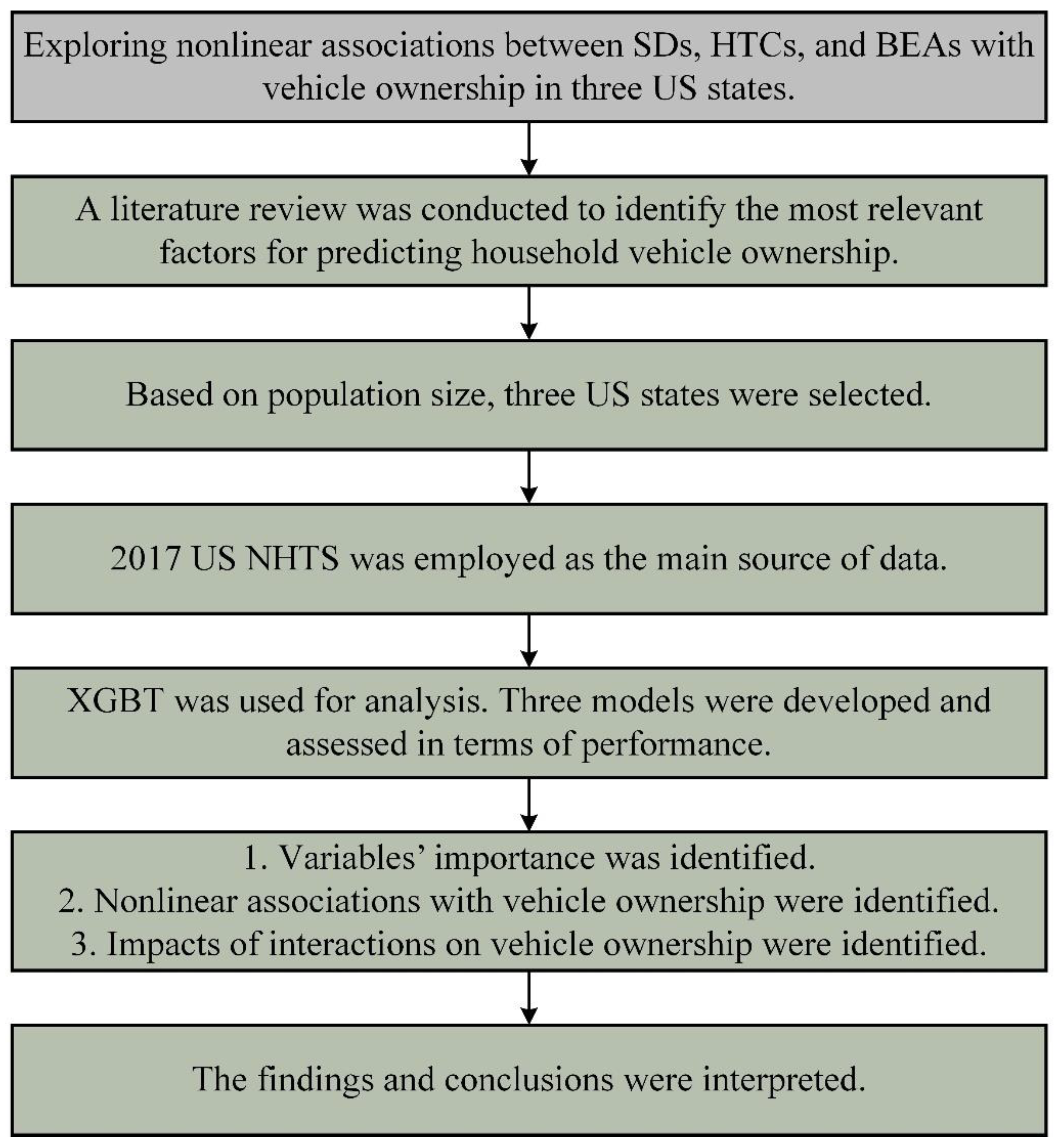
The National Household Travel Survey (NHTS) is the official source on the travel behaviour of the American public, which is carried out by the Federal Highway Administration (FHWA). These data are the singular national dataset that allows the study of personal and household travel patterns. It encompasses non-commercial travel on a daily basis in all commute modes and the features of the travellers, their households, and their vehicles. Several researchers employed these data for different purposes, including investigation of trends in taxi use and ride hailing [41,42,43], determining the occurrence of rural and urban cycling [44,45], ownership and usage assessment of unconventional fuel vehicles [46], preferences of public transportation users [47], and so on. A summary of some studies that used 2017 NHTS data is shown in Table 1.
The information presented in Table 1 reveals some shortcomings in the employment of NHTS data. First, a few studies predicted vehicle ownership using these data (e.g., [5]). Second, a very limited number of variables was used to perform the analysis by different studies. For example, no indicator of household travel characteristics (e.g., household drivers’ count, household members’ count on the trip, and household vehicle used on the trip) was used by these studies. In addition, a very limited number of built environment attributes were employed (e.g., the condition of walking and cycling infrastructure). Third, a narrow range of statistical analyses were employed by different studies. Most studies used traditional statistical analysis techniques or simple descriptive analysis. Traditional statistical methods such as regression models have strict assumptions regarding the quality of the data. In addition, these methods do not reveal the nonlinear relationships between the target variable and inputs effectively. Lastly, most studies did not differentiate between the US states or cities in terms of population size or other characteristics, which may cause some serious differences in the prediction results.

3. Methodology

3.1. Extreme Gradient Boosting (XGBT)

The XGBT model was used to determine the primary correlates of vehicle ownership and their complex relationships. XGBT was originally developed for data science [50], but it has also been used increasingly in urban planning and transportation science (e.g., [51,52,53]). The XGBT algorithm is a more regularized variant of the gradient boosting tree (GBT). In comparison to the GBT, the XGBT is better at generalization and takes less time to train [54]. Additionally, GBT and XGBT are better than traditional statistical methods (e.g., linear regression) in a number of ways. Firstly, they outperform conventional techniques in terms of data fitting. Secondly, they are capable of dealing with a variety of different sorts of data, such as categorical and continuous. Thirdly, they are insensitive to outliers and can deal with incomplete data in a flexible manner. Fourth, they help solve the problem of multicollinearity [28,55]. Furthermore, GBT and XGBT may fit any irregular connection between variables, and modelers are not required to estimate their correlations in advance. According to previous research, vehicle ownership has a nonlinear connection with the factors that are associated with it, and the complex patterns vary according to the factor [28]. While traditional statistical approaches may describe nonlinear interactions via variable transformation, the transformation is ineffective due to the irregular nonlinearity.
Owing to its advantages of high reliability and considerable flexibility, XGBT, an advanced supervised method presented by Chen and Guestrin [50] under the Gradient Boosting architecture, has been well acknowledged in Kaggle machine learning contests. XGBT’s loss function provides an extra regularization term to the objective function that attempts to smooth the ultimate learning weights and prevent over-fitting [50]. To optimize the loss function, it furthermore employs 1st or 2nd order gradient statistics. Additionally, XGBT enables row and column sample selection to address this problem, in addition to providing regular terms to avoid over-fitting. Because parallel and distributed computation allow for rapid learning, faster model exploration is conceivable. The XGBT architecture will be simply described in the subsequent paragraphs.
The aggregate of the prediction scores, f m ( a i ) of all trees can be represented as the predicted output b i ^ of the XGBT model:
b i ^ = m = 1 M f m ( a i ) , f m γ
where γ represents the regression trees’ space, M shows the regression trees’ number, and the attributes associated with sample i are denoted by a i . Every leaf node j in a particular dataset has a forecast score f m ( a i ) , commonly referred to as leaf weight. s j is the leaf weight and regression values of entire samples at this leaf node j , where j   { 1 , 2 , Q } . In the tree, the leaves’ number is shown by Q.
In machine learning issues, objective functions become the most fundamental expression, and the boosting process repeats until the objective function minimization is limited in order to estimate the number of functions used in the model, which establishes the regularized objective function as follows:
θ = i = 1 h z ( b i , b i ^ ) + α Q + 1 2 β j = 1 Q s j 2
where, h is the number of data samples provided, and i = 1 h z ( b i , b i ^ )   is the training loss function that describes how well the model fits the training sets. For punishing the model’s complexity, α Q + 1 2 β j = 1 Q s j 2 is a regularization term. The complexity cost of adding an extra leaf is α , the regularization hyper-parameter is β , and the L2 norm of leaf node j weights is s j 2 in the regularization term.
Every recently introduced tree learns from its previous trees and adjusts the residuals in the estimated values in the incremental learning procedure. As a result, all of the trees’ iteration outcomes have already been included in b ^ i ( m 1 ) . Consequently, b ^ i ( m ) can denote b ^ i ( m 1 ) + f m ( a i ) for the mth repetition, and the objective function “C” is represented as:
θ = i = 1 h z ( b i , b ^ i ( m 1 ) + f m ( a i ) ) + α Q + 1 2 β j = 1 Q s j 2
The 2nd order Taylor expansion is employed to optimize the objective effectively in the general situation for the first term loss training function.
θ m i = 1 h [ z ( b i , b ^ i ( m 1 ) + d i f m ( a i ) ) + 1 2 e i f m 2 ( a i ) ] + α Q + 1 2 β j = 1 Q s j 2
where d i = σ b ^ ( m 1 ) z ( a i , b ^ i ( m 1 ) ) and e i = σ b ^ ( m 1 ) 2   z ( a i , b ^ i ( m 1 ) ) are the loss function’s first and second-order gradient statistics. In step m, the constant terms can be subtracted to obtain the approximate objective:
θ m i = 1 h [ d i f m ( a i ) + 1 2 e i f m 2 ( a i ) ] + α Q + 1 2 β j = 1 Q s j 2
A tree is characterized as a vector of scores in branches and a leaf index mapping function that transfers an instance to a leaf j, and this procedure is written as i = 1 h f m ( a ) = j = 1 Q s j and Equation (5) can be rephrased as:
θ ( m ) = j = 1 Q [ ( i I j g i ) s j + 1 2 ( i I j e i + α ) s j 2 ] + β Q
With a fixed tree structure, quadratic function programming is used to select the perfect branch weight scores on every leaf node s j * as well as the extreme value of θ ( m ) * :
s j * = i I j d i i I j e i + β
θ ( m ) * = 1 2 j = 1 Q ( i I j d i ) 2 i I j e i + β + α Q
Equation (8) is a framework scoring function that determines the suitability of a specified vector of leaf scores. A lower value is preferable since it fits the data more effectively. In practical uses, a greedy method has been used to discover an ideal tree structure to prevent an endless number of alternative tree architectures. To develop an XGBT model, it is important to fine-tune three main XGBT parameters, including the number of trees, maximal depth, and minimum rows. Once we have trained the XGBT model, it is possible to evaluate the significance of every predictor in forecasting the response. In addition, XGBT can assess the partial dependence and association between predictors and target variables after controlling for other variables in the model. Chen and Guestrin [50] provide more thorough descriptions of the XGBT algorithm.

3.2. Data

The data come from the 2017 National Household Travel Survey (NHTS), which is conducted by the US Department of Transportation [56]. The 2017 NHTS is the 8th in a series of nationally representative cross-sectional surveys on the daily commute conducted at random times. Data were gathered from stratified random samples of households in the United States. The 2017 NHTS consists of two main processes: (1) a mail-based household recruiting survey that gathered data on the household, transport, and travel behavior; and (2) a predominantly web-based person-level retrieval survey that asked about travel on a study-assigned day.
There were 458 variables in this dataset. As previously mentioned, the main goal of this present study is to reveal the nonlinear relationship between the count of household vehicles (vehicle ownership) and sociodemographic, household travel characteristics, and built environment attributes. Consequently, based on literature, only variables that were related to household vehicle ownership were employed. These variables and their descriptions are shown in Table 2. It is worth stating that there are a limited number of built-environment variables in the NHTS. For example, only two variables, namely “reasons for not walking more = infrastructure” and “reasons for not biking more = infrastructure,” assessed the condition of walking and cycling environments. Thus, the authors considered these variables as two indicators of the condition of the walking and cycling environments. Finally, 14 variables were used as inputs in this study’s analysis, and one variable, household vehicle counts, was used as the target variable.
In this study, the authors evaluated different states with different populations. To this end, three categories of the population were considered: (1) high-population states, (2) medium-population states, and (3) low-population states. Regarding the population of US states, the authors used the United States Census Bureau [57] as the principal source. As previously stated, a list of US states that was provided by the United States Census Bureau was used. The states in this list were sorted by population. Then, this list was simply divided into the three categories. In each category, the state that had the highest population was selected. For the first category, California (CA) was selected. Missouri (MO) was selected for the second category. For the low-population states, Kansas (KS) was selected. The authors then selected 5000 samples in each state. This sampling approach prevents any bias resulting from over- or under-sampling. A flowchart of this study is presented in Figure 1.

4. Results

4.1. Nonlinear Models Development and Performance Assessment

One XGBT model was constructed for each of the three US states based on population differences in this study. These three models were developed using a set of parameters, and each of these parameters has its own value. This study employed the grid search technique to discover the optimized value of these parameters. Table 3 shows the optimum values of the XGBT models’ parameters.
To develop the XGBT models, the data were divided into training and testing sets with a ratio of 80:20. In addition, to avoid overfitting and reduce the generalization error, this study employed a 10-fold cross validation approach. The performance of these three models was evaluated using two famous performance criteria, including linear correlation (R) and mean absolute error (MAE). Equations (9) and (10) illustrate the mathematical forms of these criteria.
R = i = 1 h ( k i k ¯ i ) ( s i s ¯ i ) i = 1 n ( k i k ¯ i ) 2 ( s i s ¯ i ) 2
M A E = i = 1 n | k i s i | h
where k i and s i signify nth actual and predicted values, respectively; k ¯ i and s ¯ i indicate the average values of actual and predicted values, respectively; h shows the number of samples in the dataset. Table 4 shows the outcomes of the models’ evaluations. As can be seen, the highest training performance belonged to Kansas.

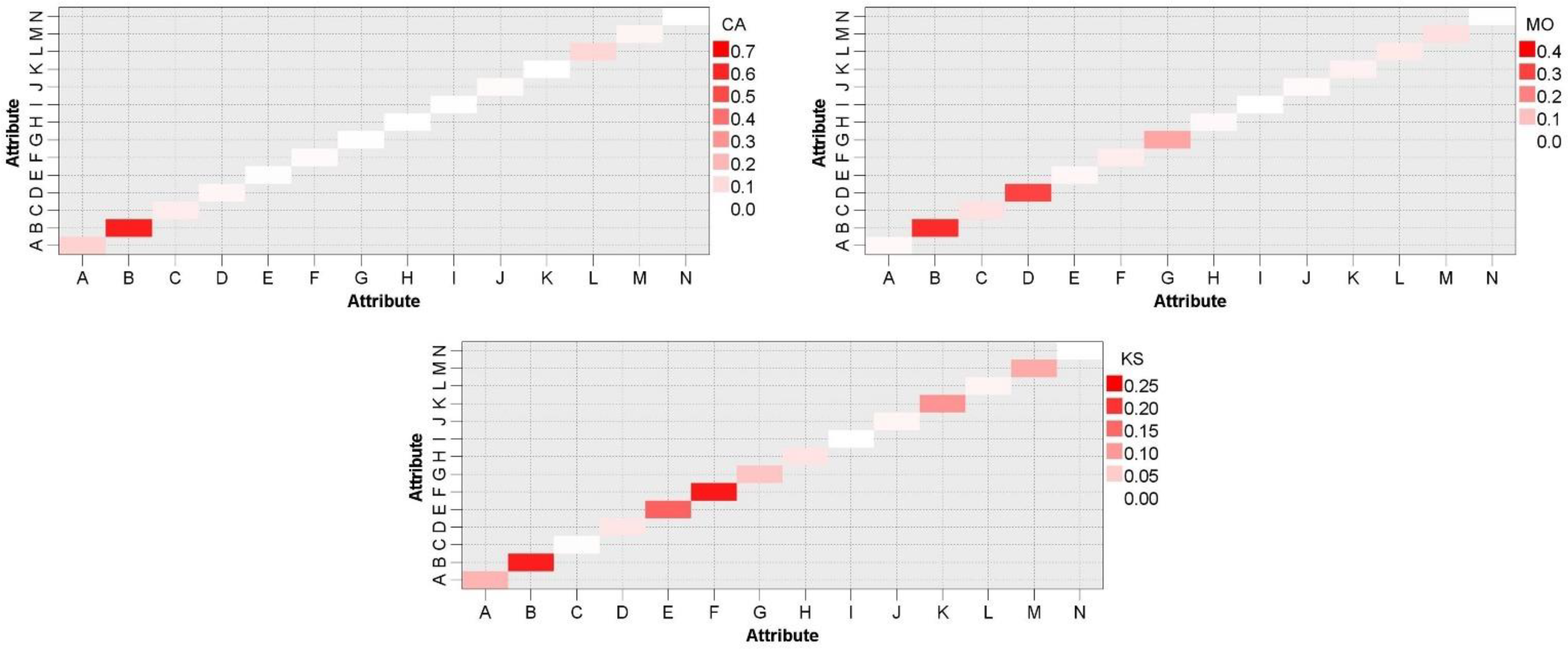
4.2. Variables’ Importance

Table 5 shows the cumulative importance (CI) of all variables in forecasting vehicle ownership. In California, household travel characteristics were the most influential factors in predicting vehicle ownership (CI: 0.62). In Missouri and Kansas, sociodemographic factors were the most important predictors of household vehicle ownership (CI: 0.53 and 0.55, respectively).
Figure 2 shows the variables’ importance in three different states of the US with different population sizes for vehicle ownership prediction. The number of drivers in a household (B) was the most important variable in California and Missouri. The importance of the number of drivers in a household was slightly lower in Kansas than that of home ownership (F).
In California, the second most important variable for the prediction of vehicle ownership was deficiencies in cycling infrastructure, followed by deficiencies in walking infrastructure. Several variables, including the count of adults in a household over the age of 18, household vehicle used on the trip, household members’ count on the trip, count of person trips on travel day, household living area (urban or rural), and count of children aged 0 to 4 in the household, had no contribution to vehicle ownership prediction in California.
Household income, which was followed by the number of adults in the household over the age of 18, was the second most influential variable in Missouri for predicting vehicle ownership. The number of children aged 0 to 4 in the household and the household vehicle used on the trip had no effect on the car ownership prediction in Missouri.
As mentioned above, in Kansas, home ownership was the most important variable, and the second most important variable for vehicle ownership forecasting was household drivers’ count, followed by household members’ count. In Kansas, the zero-contributed variables included population density, the number of children aged 0 to 4 in the household, the number of person’s trips on the travel day, and the household vehicle used on the trip.

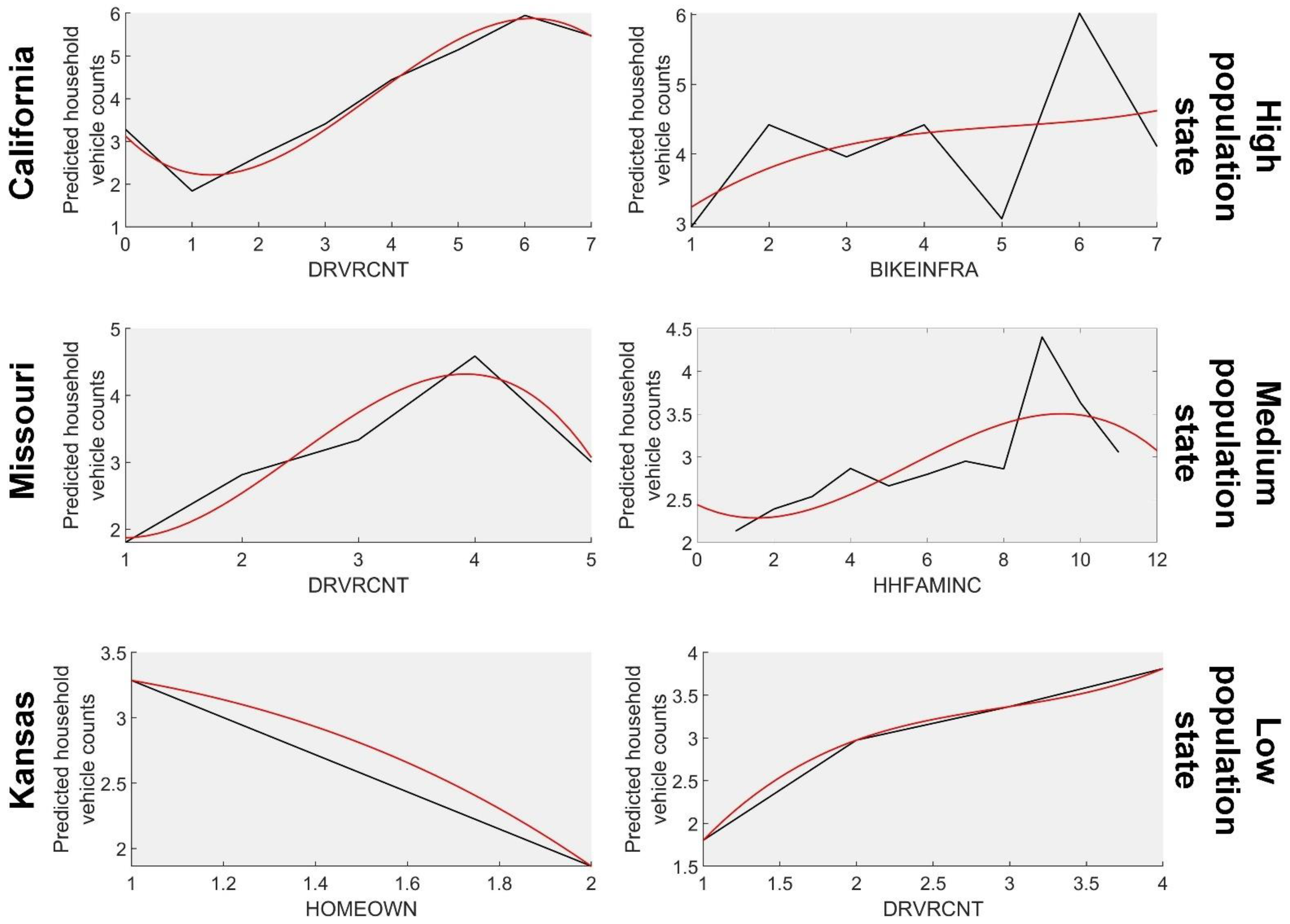
4.3. Nonlinear Associations with Car Ownership

The nonlinear associations between the predicted number of household vehicles and each state’s two most important variables are provided in this section. Figure 3 shows associations between predicted household vehicle counts and various variables in three different US states.
In California, there is a cubic relationship between the number of drivers in the household (DRVRCNT) and the household vehicle count. When the number of household drivers is within the range of two, it has a negligible effect on vehicle ownership. Beyond the threshold, it has a positive relationship with vehicle ownership. However, when the DRVRCNT exceeds six, the impact of the DRVRCNT is saturated. The cubic relationships for Missouri and Kansas are different. In Missouri, when the DRVRCNT is in the range of one to four drivers, it has a strong positive relationship with vehicle ownership. However, when the DRVRCNT is beyond four drivers, vehicle ownership starts to decrease. In Kansas, the cubic relationship between vehicle ownership and DRVRCNT is predominantly concave between 1 and 3 drivers. It seems that when the DRVRCNT exceeds four, the impact of the DRVRCNT is saturated in Kansas. Overall, the best range of DRVRCNT for cutting down on car ownership in California is between zero and two drivers. This range for Missouri and Kansas is between four and five. These findings corroborate prior research indicating that the number of drivers in a household has a considerable impact on vehicle ownership (e.g., [58,59,60,61]). No study, however, has examined the nonlinear relationship between the number of drivers in a household and vehicle ownership. As a result, the findings from this research are unique.
In the cubic relationship between vehicle ownership and deficits in cycling infrastructure (BIKEINFRA), it seems that when the BIKEINFRA is within the range of three, its impact on vehicle ownership is greater than when it is within the range of four to seven. This means that when Californian households are disappointed to find adjacent paths, trails, sidewalks, or parks, they lose their inclination to bike and switch to buying new vehicles. Several studies confirmed that providing adequate infrastructure for biking may encourage people to substitute this mode for private vehicles, but to the authors’ best knowledge, very few studies have assessed the influence of this factor on vehicle ownership. In addition, no study has specifically examined the nonlinear relationship between these factors and vehicle ownership.
In Missouri, the cubic connection between household income (HHFAMINC) and vehicle ownership indicates that when household income is between 10,000 and 14,999 USD, it has a minor influence on vehicle ownership. It has a positive correlation with vehicle ownership after the threshold is exceeded. When the HHFAMINC crosses nine (125,000–149,999 USD), the HHFAMINC’s effect becomes saturated. Several previous studies reported the positive and linear relationship between household income and vehicle ownership (e.g., [19]), but very few studies have assessed the nonlinear relationship between household income and vehicle ownership (e.g., [62]).
In Kansas, there is a strong link between home ownership (HOMEOWN) and the number of vehicles in a household, so possessing a home increases the likelihood of owning more vehicles. Since home ownership can be assumed as an indicator of family wealth, the positive relationship between home ownership and vehicle ownership is not surprising and has been reported in several previous studies (e.g., [19,62]).

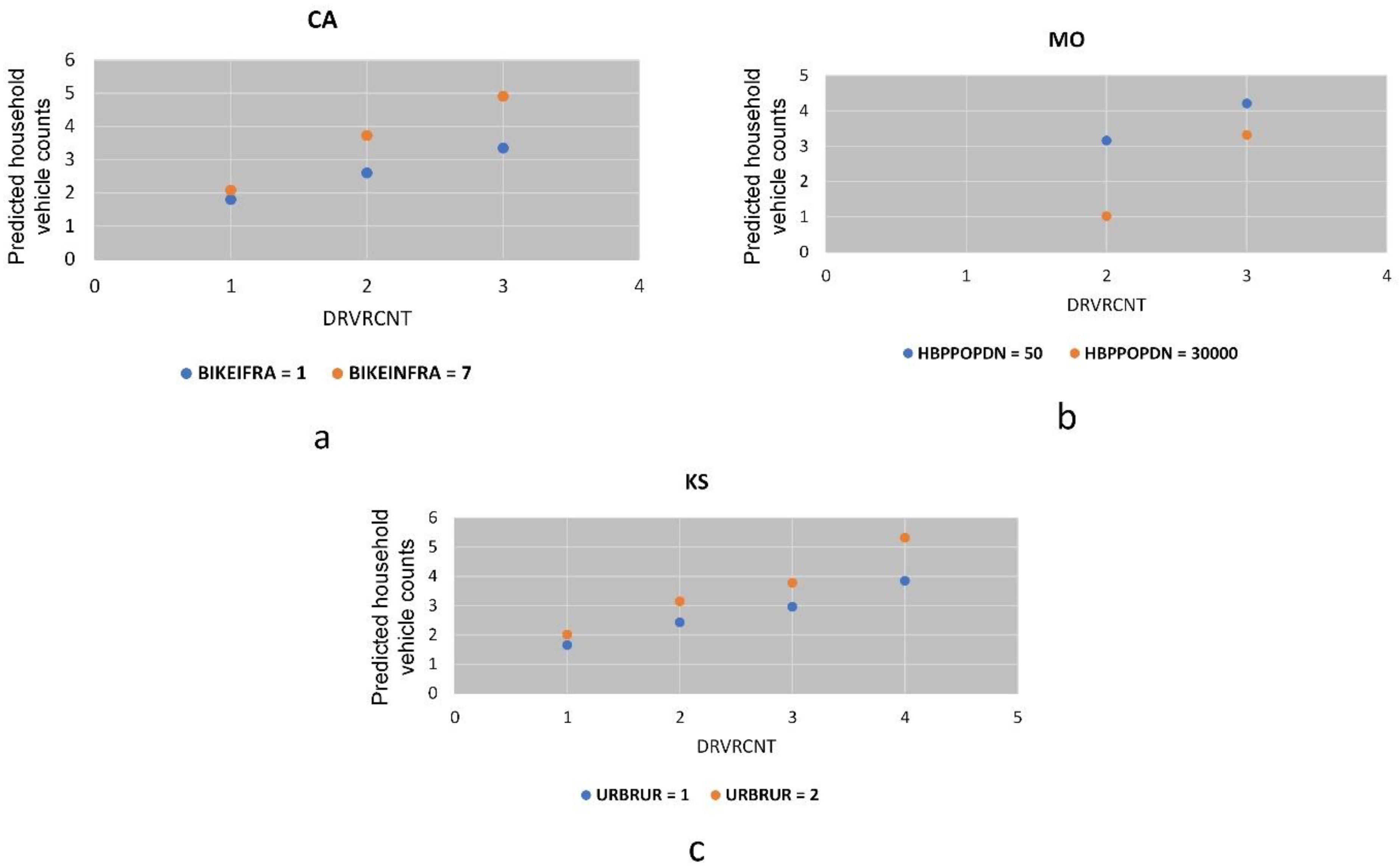
4.4. Impacts of Interactions on Vehicle Ownership

A strong positive relationship between the number of drivers in the household and vehicle ownership in all states was observed. This association implies that if the number of drivers in the household was lowered, vehicle ownership would decline substantially. This section looks at how household travel characteristics (HTCs) in each state moderate the effects of the most relevant BEA factors on vehicle ownership. BIKEINFRA was the most significant BEA variable in California, whereas HBPPOPDN and URBRUR were the most significant BEA variables in Missouri and Kansas, respectively. In all states, DRVRCNT was the most influential HTC variable. Figure 4 shows the change in predicted household vehicle counts when biking infrastructure conditions change from one to seven, a household living area changes from urban to rural, and population density increases from a category of 50 to a category of 30,000.
DRVRCT has a complex moderating influence on the relationship between the built environment and household vehicle count. For example, when biking infrastructure conditions change from one to seven, predicted household vehicle counts for all the number of drivers in a household increase, but the predicted household vehicle count growth varies by the number of drivers in a household (Figure 4a). When the number of drivers in a household is one, the smallest increment (0.28) in the number of household vehicles occurs. A medium increase (1.13) in the number of household vehicles occurs when the number of household drivers is two. Finally, when there are three people who drive in a household, the number of vehicles in the household increases the most (1.56). This suggests that the number of drivers in a household strengthens the positive influence of the deficiencies in biking infrastructure on vehicle ownership in California. The interaction effect of household living area (urban or rural) and DRVRCT on predicted household vehicle counts has a similar pattern in Kansas (Figure 4c). As living areas change from urban (1) to rural (2), vehicle ownership increases and the growth varies by the number of drivers in a household. When the household has four drivers, the largest increase in vehicle ownership occurs, suggesting that the number of drivers in a household amplifies the population density’s positive effect on vehicle ownership.
As shown in Figure 4b, in Missouri, DRVRCT also moderates the impact of population density on predicted household vehicle counts. When the population density rises from 50 to 30,000, the predicted number of household vehicles decreases as well. When a household has two drivers, the number of household vehicles decreases the most (−2.14), whereas when a household has three drivers, the number of household vehicles decreases the least (−0.89). These findings show that having more drivers in a household can lessen the negative effects of high population density on vehicle ownership.

5. Discussions

It was expected that the number of drivers in the households plays a dominant role in predicting the count of the households’ vehicles. However, very few studies have investigated the direct effects of the count of households’ drivers on vehicle ownership. Some studies [61,63] found positive associations between the total number of household vehicles, vehicle usage, and energy consumption, which can be interpreted as indirect indicators of vehicle ownership trends. A possible reason that the number of drivers in the household became the most important household travel characteristics variable in predicting vehicle ownership in the three US states could be the direct and positive relationship between this variable and the number of adults in the households. Having more adults in a household means that people have different responsibilities and can travel independently. Thus, each adult household member may require their own vehicle, which cannot be shared with others due to time constraints. The importance of the number of drivers in the household in all three states shows that this variable is a determinant of households’ vehicle ownership regardless of the state’s population size.
Many previous studies have confirmed that providing adequate cycling and walking facilities encourages people to use these modes more frequently (e.g., [64,65,66]). At least for recreational or short trips, this may also encourage people to replace vehicles with walking and cycling [67,68]. These may be the causes of emerging deficiencies in cycling facilities as an important predictor of vehicle ownership in California. Having poor cycling facilities may increase the tendency of adult household members to buy more vehicles. According to The League of American Bicyclists [69], among all the US states, California, Missouri, and Kansas are ranked 4, 35, and 37, respectively, in terms of their suitability for cycling. Thus, the emergence of biking infrastructure conditions in California as an important factor is sensible. California has better conditions in terms of infrastructure and funding, education and encouragement, legislation and enforcement, policies and programs, and evaluation and planning than the other two states [69]. In addition, other factors such as biking culture, topography, and integration of walking and cycling facilities with public transport services can make a difference among the US states in terms of adoption of walking and biking instead of using private vehicles.

5.1. Findings’ Implications

The practical examinations in the earlier sections accomplished the investigation objectives by revealing the characteristics of households that belonged to different US states and different populations. The results have significant implications for households’ vehicle ownership. This paper’s analysis clearly showed that the number of drivers in the household and deficiencies in cycling infrastructure heavily impacted the household vehicle numbers. Moreover, the results revealed that these variables are determinants of household vehicle ownership regardless of the state’s population. Thus, to discourage households from possessing multiple vehicles, any policy that reduces the impact of these variables is desired.
The members of the household have varying life commitments and travel requirements. As a result, considering all family members’ needs and encouraging them to share their vehicles with other family members rather than purchasing more vehicles is a daunting task. However, some solutions, including using a minivan, flexible working time, using micro-mobility for first and last connections, and sending children to schools near the house, can be used to reduce the number of drivers in the household.
Improvements to the cycling infrastructure in all states (especially Kansas) should be at the center of attention. Some measures include the construction of paths, trails, or parks near housing units; the construction of sidewalks along all local and arterial streets; and the consistent assessment of sidewalks to ensure that they can serve all people, regardless of physical ability [64].
In most states, regardless of their population, the BEAs could not have the highest cumulative contribution to household vehicle ownership. Most BEAs had a minor impact on reducing vehicle ownership growth in the short term, but a BEA that made alternate modes of transportation competitive with a vehicle may have created a positive circle between the BEA and vehicle ownership in the long term. However, since transportation infrastructure and construction persist for years, a motorized-oriented urban layout is difficult to reverse once it has been established. Moreover, the motorized-oriented metropolitan structure will foster people’s intention to purchase vehicles, which will be harmful to sustainable mobility.

5.2. Limitations

The study has significant limitations. First, the NHTS dataset is one of the largest household travel survey datasets in the world. However, its built environment indicators are limited. Some of these overlooked factors are location and transit accessibility (e.g., distance to the central business district and distance to the nearest metro/bus stop). Thus, future studies can employ other datasets containing more built-environment attributes and apply the XGBT method to perform their analysis. Additionally, it is suggested that the NHTS consider the factors mentioned above since these factors allow researchers to conduct a more comprehensive study regarding the issue of vehicle ownership in the US. Second, the NHTS includes items regarding reasons for not walking and biking. However, there are no items regarding the deficiencies in public transportation, particularly public buses. Future studies may complement the NHTS dataset with field observations on public transport infrastructure conditions. Finally, the authors believe that a sample of 5000 per state were enough to analyze the nonlinear relationship between vehicle ownership and other variables. However, future studies can use a larger sample to perform their analysis.

6. Conclusions

By means of data from the US National Household Travel Survey, this research utilized an extreme gradient boosting tree (XGBT) model to investigate the importance of sociodemographic factors, the HTCs, and the BEAs to vehicle ownership and their nonlinear associations with vehicle ownership. It is one of the few studies that look at how key HTCs moderate the effects of important BEAs on vehicle ownership in three different states in the United States with different populations. However, this study could not find a substantial difference in the results based on the states’ populations. The main findings of this study for each state are as follows:
  • In California, the predictability of vehicle ownership was driven by household travel characteristics (CI: 0.62). In this state, the number of drivers in a household and the deficiencies in cycling infrastructure were the two most important factors in predicting vehicle ownership.
  • In Missouri, sociodemographic factors were dominant factors in predicting vehicle ownership (CI: 0.53). The number of drivers in a household and household income were the two most important predictors of vehicle ownership in Missouri.
  • In Kansas, sociodemographic factors were the most influential factors in predicting vehicle ownership (CI: 0.55). Home ownership and the number of drivers in a household were the most influential factors in vehicle ownership in Kansas.
The outcomes demonstrate that the number of drivers in a household plays a dominant role in households’ choice of vehicle ownership in the three US states. Crowded families with many drivers are more likely to possess more vehicles. In addition, deficiencies in the cycling infrastructure are another vital determinant of vehicle ownership in California. These two variables in California are the most significant predictors, accounting for 0.74 of the predictive capabilities. Identifying effective strategies to discourage households’ drivers from buying new vehicles and improving the cycling infrastructure is key to sustainable transport in these states.
Policymakers could utilize land use and transport strategies to transform the built environment. The BEAs have a modest impact on vehicle ownership, and several BEAs may be used as proxies for the number of drivers in a household. Because practically all BEAs have a minor impact on their own, policymakers will need a combination of tactics if they intend to restrict vehicle ownership using land use and transport policy.
Some of the findings of this study are unique. For example, the nonlinear relationship between vehicle ownership and the number of drivers in a household has not been assessed by the previous studies. Thus, policymakers can use the findings of this study (thresholds, relationships, and interaction effects) to propose strategies to cope with the growth of vehicle ownership in the US.
Several factors are only connected with vehicle ownership when they fall within a specified range. It can result in a subjective interpretation of the associations between variables if the nonlinear associations are overlooked. This can lead planners and researchers to misjudge the significance of these variables and inaccurately signify their associations with vehicle ownership. More significantly, these ranges provide policymakers with recommendations about how to efficiently reduce the increase in vehicle ownership.
The findings of this research also showed that the XGBT can be successfully applied to reveal the complex relationships between the input variables and the target variables. Future studies can use this method to solve other issues in transportation science. To get more accurate results, they can combine the XGBT with other machine learning techniques, such as those that were proposed in Kumar et al. [70], Golilarz et al. [71], Golilarz et al. [72], Najafi Moghaddam Gilani et al. [73], Gilani et al. [74], and Tao et al. [75].

Author Contributions

Conceptualization, T.M., M.A. (Mahdi Aghaabbasi), and M.A. (Mujahid Ali); investigation, T.M., M.A. (Mahdi Aghaabbasi), and M.A. (Mujahid Ali); formal analysis, M.A. (Mahdi Aghaabbasi), and M.A. (Mujahid Ali); methodology, M.A. (Mahdi Aghaabbasi); software, M.A. (Mahdi Aghaabbasi), and M.A. (Mujahid Ali); writing—original draft, T.M., M.A. (Mahdi Aghaabbasi), and M.A. (Mujahid Ali); writing—review and editing, T.M., M.A. (Mahdi Aghaabbasi), M.A. (Mujahid Ali), A.J., A.M.M., and A.M.; supervision, R.Z.; funding acquisition, A.M.M., and A.M. All authors have read and agreed to the published version of the manuscript.

Funding

This research received no external funding.

Institutional Review Board Statement

Not applicable.

Informed Consent Statement

Not applicable.

Data Availability Statement

Not applicable.

Acknowledgments

Social Science Planning Fund of Liaoning Province (L20AXW001).

Conflicts of Interest

The authors declare no conflict of interest.

References

  1. Bureau of Transportation Statistics. National Household Travel Survey Daily Travel Quick Facts. Available online: https://www.bts.gov/statistical-products/surveys/national-household-travel-survey-daily-travel-quick-facts (accessed on 1 February 2022).
  2. Handy, S.L.; Boarnet, M.G.; Ewing, R.; Killingsworth, R.E. How the built environment affects physical activity: Views from urban planning. Am. J. Prev. Med. 2002, 23, 64–73. [Google Scholar] [CrossRef]
  3. Zhao, P.; Zhang, Y. Travel behaviour and life course: Examining changes in car use after residential relocation in Beijing. J. Transp. Geogr. 2018, 73, 41–53. [Google Scholar] [CrossRef]
  4. Zegras, C. The built environment and motor vehicle ownership and use: Evidence from Santiago de Chile. Urban Stud. 2010, 47, 1793–1817. [Google Scholar] [CrossRef]
  5. Sabouri, S.; Tian, G.; Ewing, R.; Park, K.; Greene, W. The built environment and vehicle ownership modeling: Evidence from 32 diverse regions in the US. J. Transp. Geogr. 2021, 93, 103073. [Google Scholar] [CrossRef]
  6. Ao, Y.; Chen, C.; Yang, D.; Wang, Y. Relationship between rural built environment and household vehicle ownership: An empirical analysis in rural Sichuan, China. Sustainability 2018, 10, 1566. [Google Scholar] [CrossRef] [Green Version]
  7. Kim, S.H.; Mokhtarian, P.L. Taste heterogeneity as an alternative form of endogeneity bias: Investigating the attitude-moderated effects of built environment and socio-demographics on vehicle ownership using latent class modeling. Transp. Res. Part A Policy Pract. 2018, 116, 130–150. [Google Scholar] [CrossRef]
  8. Rahul, T.; Verma, A. The influence of stratification by motor-vehicle ownership on the impact of built environment factors in Indian cities. J. Transp. Geogr. 2017, 58, 40–51. [Google Scholar] [CrossRef]
  9. Ruas, E.B. The Influence of Shared Mobility and Transportation Policies on Vehicle Ownership: Analysis of Multifamily Residents in Portland, Oregon. Ph.D. Thesis, Portland State University, Portland, OR, USA, 2019. [Google Scholar]
  10. Li, J.; Walker, J.L.; Srinivasan, S.; Anderson, W.P. Modeling private car ownership in China: Investigation of urban form impact across megacities. Transp. Res. Rec. 2010, 2193, 76–84. [Google Scholar] [CrossRef]
  11. Song, S.; Diao, M.; Feng, C.-C. Effects of pricing and infrastructure on car ownership: A pseudo-panel-based dynamic model. Transp. Res. Part A Policy Pract. 2021, 152, 115–126. [Google Scholar] [CrossRef]
  12. Dargay, J.M.; Madre, J.-L.; Berri, A. Car ownership dynamics seen through the follow-up of cohorts: Comparison of France and the United Kingdom. Transp. Res. Rec. 2000, 1733, 31–38. [Google Scholar] [CrossRef]
  13. Yang, Z.; Jia, P.; Liu, W.; Yin, H. Car ownership and urban development in Chinese cities: A panel data analysis. J. Transp. Geogr. 2017, 58, 127–134. [Google Scholar] [CrossRef]
  14. Ma, Z. Multi-level Probabilistic Model for Population Synthesis and Vehicle Ownership Modeling Based on Samples with Missing Values. Master’s Thesis, McGill University, Montreal, QC, Canada, 2021. [Google Scholar]
  15. Cirillo, C.; Liu, Y. Vehicle ownership modeling framework for the state of Maryland: Analysis and trends from 2001 and 2009 NHTS data. J. Urban Plan. Dev. 2013, 139, 1–11. [Google Scholar] [CrossRef] [Green Version]
  16. Chu, M.Y.; Law, T.H.; Hamid, H.; Law, S.H.; Lee, J.C. Examining the effects of urbanization and purchasing power on the relationship between motorcycle ownership and economic development: A panel data. Int. J. Transp. Sci. Technol. 2020; in press. [Google Scholar] [CrossRef]
  17. Dargay, J.; Hanly, M. Volatility of car ownership, commuting mode and time in the UK. Transp. Res. Part A: Policy Pract. 2007, 41, 934–948. [Google Scholar] [CrossRef] [Green Version]
  18. Bhat, C.R.; Paleti, R.; Pendyala, R.M.; Lorenzini, K.; Konduri, K.C. Accommodating Immigration Status and Self-Selection Effects in a Joint Model of Household Auto Ownership and Residential Location Choice. Transp. Res. Rec. 2013, 2382, 142–150. [Google Scholar] [CrossRef] [Green Version]
  19. Li, S.; Zhao, P. Exploring car ownership and car use in neighborhoods near metro stations in Beijing: Does the neighborhood built environment matter? Transp. Res. Part D Transp. Environ. 2017, 56, 1–17. [Google Scholar] [CrossRef]
  20. Huang, X.; Cao, X.J.; Yin, J.; Cao, X. Effects of metro transit on the ownership of mobility instruments in Xi’an, China. Transp. Res. Part D: Transp. Environ. 2017, 52, 495–505. [Google Scholar] [CrossRef] [Green Version]
  21. Matas, A.; Raymond, J.-L.; Roig, J.-L. Car ownership and access to jobs in Spain. Transp. Res. Part A Policy Pract. 2009, 43, 607–617. [Google Scholar] [CrossRef] [Green Version]
  22. Tyrinopoulos, Y.; Antoniou, C. Factors affecting modal choice in urban mobility. Eur. Transp. Res. Rev. 2013, 5, 27–39. [Google Scholar] [CrossRef] [Green Version]
  23. Sabouri, S.; Brewer, S.; Ewing, R. Exploring the relationship between ride-sourcing services and vehicle ownership, using both inferential and machine learning approaches. Landsc. Urban Plan. 2020, 198, 103797. [Google Scholar] [CrossRef]
  24. Holtzclaw, J.; Clear, R.; Dittmar, H.; Goldstein, D.; Haas, P. Location efficiency: Neighborhood and socio-economic characteristics determine auto ownership and use-studies in Chicago, Los Angeles and San Francisco. Transp. Plan. Technol. 2002, 25, 1–27. [Google Scholar] [CrossRef]
  25. Shay, E.; Khattak, A.J. Household travel decision chains: Residential environment, automobile ownership, trips and mode choice. Int. J. Sustain. Transp. 2012, 6, 88–110. [Google Scholar] [CrossRef]
  26. Ding, C.; Cao, X.; Dong, M.; Zhang, Y.; Yang, J. Non-linear relationships between built environment characteristics and electric-bike ownership in Zhongshan, China. Transp. Res. Part D Transp. Environ. 2019, 75, 286–296. [Google Scholar] [CrossRef]
  27. Wang, X.; Yin, C.; Zhang, J.; Shao, C.; Wang, S. Nonlinear effects of residential and workplace built environment on car dependence. J. Transp. Geogr. 2021, 96, 103207. [Google Scholar] [CrossRef]
  28. Zhang, W.; Zhao, Y.; Cao, X.J.; Lu, D.; Chai, Y. Nonlinear effect of accessibility on car ownership in Beijing: Pedestrian-scale neighborhood planning. Transp. Res. Part D Transp. Environ. 2020, 86, 102445. [Google Scholar] [CrossRef]
  29. Bargegol, I.; Najafi Moghaddam Gilani, V.; Jamshidpour, F. Relationship between Pedestrians’ Speed, Density and Flow Rate of Crossings through Urban Intersections (Case Study: Rasht Metropolis) (RESEARCH NOTE). Int. J. Eng. 2017, 30, 1814–1821. [Google Scholar]
  30. Bargegol, I.; Amlashi, A.T.; Gilani, V.N.M. Estimation the Saturation Flow Rate at Far-side and Nearside Legs of Signalized Intersections—Case Study: Rasht City. Procedia Eng. 2016, 161, 226–234. [Google Scholar] [CrossRef] [Green Version]
  31. Zhao, T.H.; Khan, M.I.; Chu, Y.M. Artificial neural networking (ANN) analysis for heat and entropy generation in flow of non-Newtonian fluid between two rotating disks. Math. Methods Appl. Sci. 2021. Available online: https://onlinelibrary.wiley.com/doi/10.1002/mma.7310 (accessed on 1 January 2022). [CrossRef]
  32. Zhao, T.-H.; Shi, L.; Chu, Y.-M. Convexity and concavity of the modified Bessel functions of the first kind with respect to Hölder means. Rev. Real Acad. Cienc. Exactas Fís. Nat. Ser. A Matemáticas 2020, 114, 96. [Google Scholar] [CrossRef]
  33. Wang, M.-K.; Hong, M.-Y.; Xu, Y.-F.; Shen, Z.-H.; Chu, Y.-M. Inequalities for generalized trigonometric and hyperbolic functions with one parameter. J. Math. Inequal 2020, 14, 1–21. [Google Scholar] [CrossRef]
  34. Zha, T.-H.; Castillo, O.; Jahanshahi, H.; Yusuf, A.; Alassafi, M.O.; Alsaadi, F.E.; Chu, Y.-M. A fuzzy-based strategy to suppress the novel coronavirus (2019-NCOV) massive outbreak. Appl. Comput. Math. 2021, 20, 160–176. [Google Scholar]
  35. Zhao, T.-H.; Wang, M.-K.; Hai, G.-J.; Chu, Y.-M. Landen inequalities for Gaussian hypergeometric function. Rev. Real Acad. Cienc. Exactas Físicas Nat. Ser. A Matemáticas 2022, 116, 53. [Google Scholar] [CrossRef]
  36. Iqbal, M.A.; Wang, Y.; Miah, M.M.; Osman, M.S. Study on Date–Jimbo–Kashiwara–Miwa Equation with Conformable Derivative Dependent on Time Parameter to Find the Exact Dynamic Wave Solutions. Fractal Fract. 2022, 6, 4. [Google Scholar] [CrossRef]
  37. Zhao, T.-H.; Wang, M.-K.; Chu, Y.-M. Monotonicity and convexity involving generalized elliptic integral of the first kind. Rev. Real Acad. Cienc. Exactas Fís. Nat. Ser. A Matemáticas 2021, 115, 46. [Google Scholar] [CrossRef]
  38. Zhao, T.-H.; He, Z.-Y.; Chu, Y.-M. On some refinements for inequalities involving zero-balanced hypergeometric function. AIMS Math 2020, 5, 6479–6495. [Google Scholar] [CrossRef]
  39. Zhao, T.-H.; Wang, M.-K.; Chu, Y.-M. A sharp double inequality involving generalized complete elliptic integral of the first kind. AIMS Math 2020, 5, 4512–4528. [Google Scholar] [CrossRef]
  40. Song, Y.-Q.; Zhao, T.-H.; Chu, Y.-M.; Zhang, X.-H. Optimal evaluation of a Toader-type mean by power mean. J. Inequalities Appl. 2015, 2015, 408. [Google Scholar] [CrossRef] [Green Version]
  41. Conway, M.W.; Salon, D.; King, D.A. Trends in taxi use and the advent of ridehailing, 1995–2017: Evidence from the US National Household Travel Survey. Urban Sci. 2018, 2, 79. [Google Scholar] [CrossRef] [Green Version]
  42. Jiao, J.; Bischak, C.; Hyden, S. The impact of shared mobility on trip generation behavior in the US: Findings from the 2017 National Household Travel Survey. Travel Behav. Soc. 2020, 19, 1–7. [Google Scholar] [CrossRef]
  43. Das, V. Does Adoption of Ridehailing Result in More Frequent Sustainable Mobility Choices? An Investigation Based on the National Household Travel Survey (NHTS) 2017 Data. Smart Cities 2020, 3, 385–400. [Google Scholar] [CrossRef]
  44. Tribby, C.P.; Tharp, D.S. Examining urban and rural bicycling in the United States: Early findings from the 2017 National Household Travel Survey. J. Transp. Health 2019, 13, 143–149. [Google Scholar] [CrossRef]
  45. Porter, A.K.; Kontou, E.; McDonald, N.C.; Evenson, K.R. Perceived barriers to commuter and exercise bicycling in US adults: The 2017 National Household Travel Survey. J. Transp. Health 2020, 16, 100820. [Google Scholar] [CrossRef]
  46. Li, X.; Liu, C.; Jia, J. Ownership and usage analysis of alternative fuel vehicles in the United States with the 2017 national household travel survey data. Sustainability 2019, 11, 2262. [Google Scholar] [CrossRef] [Green Version]
  47. Jin, H.; Yu, J. Gender Responsiveness in Public Transit: Evidence from the 2017 US National Household Travel Survey. J. Urban Plan. Dev. 2021, 147, 04021021. [Google Scholar] [CrossRef]
  48. Godfrey, J.; Polzin, S.E.; Roessler, T. Public Transit in America: Observations from the 2017 National Household Travel Survey; Center for Urban Transportation Research: Tampa, FL, USA, 2019. [Google Scholar]
  49. Sadeghvaziri, E.; Tawfik, A. Using the 2017 National Household Travel Survey Data to Explore the Elderly’s Travel Patterns. In Proceedings of the International Conference on Transportation and Development, Seattle, WA, USA, 26–29 May 2020; pp. 86–94. [Google Scholar]
  50. Chen, T.; Guestrin, C. XGBoost: A scalable tree boosting system. In Proceedings of the 22nd ACM SIGKDD International Conference on Knowledge Discovery and Data Mining, San Francisco, CA, USA, 13–17 August 2016; ACM: New York, NY, USA, 2016; Volume 10, pp. 785–794. [Google Scholar]
  51. Hak Lee, E.; Kim, K.; Kho, S.-Y.; Kim, D.-K.; Cho, S.-H. Estimating Express Train Preference of Urban Railway Passengers Based on Extreme Gradient Boosting (XGBoost) using Smart Card Data. Transp. Res. Rec. 2021, 2675, 64–76. [Google Scholar] [CrossRef]
  52. Mahmoud, N.; Abdel-Aty, M.; Cai, Q.; Yuan, J. Predicting cycle-level traffic movements at signalized intersections using machine learning models. Transp. Res. Part C Emerg. Technol. 2021, 124, 102930. [Google Scholar] [CrossRef]
  53. Cai, Q.; Abdel-Aty, M.; Zheng, O.; Wu, Y. Applying machine learning and google street view to explore effects of drivers’ visual environment on traffic safety. Transp. Res. Part C Emerg. Technol. 2022, 135, 103541. [Google Scholar] [CrossRef]
  54. Kaur, H.; Kumar, M. Offline handwritten Gurumukhi word recognition using eXtreme Gradient Boosting methodology. Soft Comput. 2021, 25, 4451–4464. [Google Scholar] [CrossRef]
  55. Ding, C.; Cao, X.J.; Næss, P. Applying gradient boosting decision trees to examine non-linear effects of the built environment on driving distance in Oslo. Transp. Res. Part A Policy Pract. 2018, 110, 107–117. [Google Scholar] [CrossRef]
  56. Transportation Secure Data Center. 2017 National Household Travel Survey—California; National Household Travel Survey: Sacramento, CA, USA, 2019. [Google Scholar]
  57. United States Census Bureau. Most Populous. 2017. Available online: https://www.census.gov/topics/population.html/ (accessed on 2 January 2022).
  58. Potoglou, D.; Kanaroglou, P.S. Modelling car ownership in urban areas: A case study of Hamilton, Canada. J. Transp. Geogr. 2008, 16, 42–54. [Google Scholar] [CrossRef]
  59. Kim, H.S.; Kim, E. Effects of Public Transit on Automobile Ownership and Use in Households of the USA. In Review of Urban & Regional Development Studies: Journal of the Applied Regional Science Conference; Blackwell Publishing: Oxford, UK; Boston, MA, USA, 2004. [Google Scholar]
  60. Chu, Y.-L. Automobile Ownership Analysis Using Ordered Probit Models. Transp. Res. Rec. 2002, 1805, 60–67. [Google Scholar] [CrossRef]
  61. Brownstone, D.; Golob, T.F. The impact of residential density on vehicle usage and energy consumption. J. Urban Econ. 2009, 65, 91–98. [Google Scholar] [CrossRef] [Green Version]
  62. Shao, Q.; Zhang, W.; Cao, X.J.; Yang, J. Nonlinear and interaction effects of land use and motorcycles/E-bikes on car ownership. Transp. Res. Part D Transp. Environ. 2022, 102, 103115. [Google Scholar] [CrossRef]
  63. Liu, F.; Zhao, F.; Liu, Z.; Hao, H. The Impact of Purchase Restriction Policy on Car Ownership in China’s Four Major Cities. J. Adv. Transp. 2020, 2020, 7454307. [Google Scholar] [CrossRef]
  64. Aghaabbasi, M.; Moeinaddini, M.; Shah, M.Z.; Asadi-Shekari, Z. A new assessment model to evaluate the microscale sidewalk design factors at the neighbourhood level. J. Transp. Health 2017, 5, 97–112. [Google Scholar] [CrossRef]
  65. Buehler, R. Determinants of bicycle commuting in the Washington, DC region: The role of bicycle parking, cyclist showers, and free car parking at work. Transp. Res. Part D Transp. Environ. 2012, 17, 525–531. [Google Scholar] [CrossRef]
  66. Piatkowski, D.P.; Marshall, W.E. Not all prospective bicyclists are created equal: The role of attitudes, socio-demographics, and the built environment in bicycle commuting. Travel Behav. Soc. 2015, 2, 166–173. [Google Scholar] [CrossRef]
  67. Verma, A.; Vajjarapu, H.; Thuluthiyil Manoj, M. Planning and Usage Analysis of Bike Sharing System in a University Campus. In Proceedings of the Recent Advances in Traffic Engineering, Singapore, 29 August 2020; pp. 339–349. [Google Scholar]
  68. Torcat, A.; McCray, T.; Durden, T. Changing Perceptions of Cycling in the African American Community to Encourage Participation in a Sport that Promotes Health in Adults; Southwest Region University Transportation Center (US): College Station, TX, USA, 2015. [Google Scholar]
  69. The League of American Bicyclists. Bicycle-Friendly. Available online: https://rosap.ntl.bts.gov/view/dot/29321 (accessed on 3 January 2022).
  70. Kumar, R.; Khan, A.A.; Kumar, J.; Zakria; Golilarz, N.A.; Zhang, S.; Ting, Y.; Zheng, C.; Wang, W. Blockchain-Federated-Learning and Deep Learning Models for COVID-19 Detection Using CT Imaging. IEEE Sens. J. 2021, 21, 16301–16314. [Google Scholar] [CrossRef]
  71. Golilarz, N.A.; Mirmozaffari, M.; Gashteroodkhani, T.A.; Ali, L.; Dolatsara, H.A.; Boskabadi, A.; Yazdi, M. Optimized Wavelet-Based Satellite Image De-Noising With Multi-Population Differential Evolution-Assisted Harris Hawks Optimization Algorithm. IEEE Access 2020, 8, 133076–133085. [Google Scholar] [CrossRef]
  72. Golilarz, N.A.; Addeh, A.; Gao, H.; Ali, L.; Roshandeh, A.M.; Munir, H.M.; Khan, R.U. A New Automatic Method for Control Chart Patterns Recognition Based on ConvNet and Harris Hawks Meta Heuristic Optimization Algorithm. IEEE Access 2019, 7, 149398–149405. [Google Scholar] [CrossRef]
  73. Najafi Moghaddam Gilani, V.; Hosseinian, S.M.; Ghasedi, M.; Nikookar, M. Data-Driven Urban Traffic Accident Analysis and Prediction Using Logit and Machine Learning-Based Pattern Recognition Models. Math. Probl. Eng. 2021, 2021, 9974219. [Google Scholar] [CrossRef]
  74. Gilani, V.N.M.; Hosseinian, S.M.; Hamedi, G.H.; Safari, D. Presentation of predictive models for two-objective optimization of moisture and fatigue damages caused by deicers in asphalt mixtures. J. Test. Eval. 2021, 49, 1–22. [Google Scholar]
  75. Tao, W.; Aghaabbasi, M.; Ali, M.; Almaliki, A.H.; Zainol, R.; Almaliki, A.A.; Hussein, E.E. An Advanced Machine Learning Approach to Predicting Pedestrian Fatality Caused by Road Crashes: A Step toward Sustainable Pedestrian Safety. Sustainability 2022, 14, 2436. [Google Scholar] [CrossRef]
Figure 1. Flowchart of this study.
Sustainability 14 03395 g001
Figure 2. Importance of variables by different US states: (A = BIKEINFRA; B = DRVRCNT; C = HBPPOPDN; D = HHFAMINC; E = HHSIZE; F = HOMEOWN; G = NUMADLT; H = TRPHHACC; I = TRPHHVEH; J = URBANSIZE; K = URBRUR; L = WALK_DEF; M = WRKCOUNT; N = YOUNGCHILD).
Sustainability 14 03395 g002
Figure 3. Relationships between predicted household vehicle counts and various variables in three different US states.
Sustainability 14 03395 g003
Figure 4. Relationships between essential BEA variables in each state and vehicle ownership variations moderated by key HTC variables. (a): Increase of vehicle ownership when condition of walking infrastructure changes from 1 to 7; (b): decrease in vehicle ownership as population density increases from 50 to 50,000 people; (c): increase in vehicle ownership as people’s living environments shift from urban to rural.
Sustainability 14 03395 g004
Table 1. Some recent studies that employed 2017 NHTS data.
StudyStudy AimVariables UsedAnalysis Technique(s)
Conway, Salon, and King [41]To report on taxi usage patterns and the rise of ride-hailing services.Sociodemographic, personal tripsDescriptive analysis, logistic regression
Godfrey et al. [48]To address some of the most pressing concerns affecting public transit.SociodemographicDescriptive analysis
Li, Liu, and Jia [46]To look at the current state of conventional car ownership and usage, as well as renewable fuels vehicle ownership and consumption.SociodemographicDescriptive analysis
Tribby and Tharp [44]To determine the prevalence of cycling patterns by city, as well as the features that best distinguish cyclists from non-cyclists.SociodemographicLogistic regression
Das [43]To determine the impact of ride hailing service uptake on sustainable mobility options.Sociodemographic, built environment attributesLogistic regression
Jiao, Bischak, and Hyden [42]To determine the effect of shared mobility on trip production.Sociodemographic, built environment attributesNegative binomial (NB) model
Porter, Kontou, McDonald, and Evenson [45]To describe the overall impediments to riding as self-reported.SociodemographicDescriptive analysis
Sadeghvaziri and Tawfik [49]To learn more about how the elderly travel.SociodemographicDescriptive analysis
Jin and Yu [47]To gain a better understanding of the fundamental reasons why people avoid taking public transportation by looking at the viewpoints of various users.Sociodemographic, descriptive analysis
Sabouri, Tian, Ewing, Park, and Greene [5]Using regional household travel data and constructed environmental characteristics from 32 regions across the United States, vehicle ownership models were assessed.Sociodemographic, built environment attributesLogistic regression
Table 2. Variables’ description.
VariableDescriptionValue
Independent variable
HHVEHCNTHousehold vehicles’ count[0–12]
Sociodemographic (SD)
HHFAMINCHousehold income ($)(1) <10,000; (2) 10,000–14,999; (3) 15,000–24,999; (4) 25,000–34,999; (5) 35,000–49,999; (6) 50,000–74,999; (7) 75,000–99,999; (8) 100,000–124,999; (9) 125,000–149,999; (10) 150,000–199,999; (11) >200,000
HHSIZEHousehold members’ count[1–13]
HOMEOWNHome ownership(1) own; (2) rent
NUMADLTCount of adults in the household over the age of 18[1–10]
WRKCOUNTHousehold workers’ count[1–7]
YOUNGCHILDCount of children aged 0 to 4 in the household[1–5]
Household travel characteristics (HTC)
DRVRCNTHousehold drivers’ count[0–9]
TRPHHACCHousehold members’ count on the trip[0–10]
TRPHHVEHHousehold vehicle used on trip(1) yes; (2) no
Built environment attributes (BEA)
BIKEINFRADeficiencies in cycling infrastructure *(1) no adjacent paths or trails; (2) no sidewalks or sidewalks are in poor condition; (3) no adjacent parks; (4) 1 and 2; (5) 1 and 3; (6) 2 and 3; (7) 1, 2, and 3
HBPPOPDNCategory of population density (persons per sqmi) in the household’s home census block group50 = 0–99; 300 = 100–499; 750 = 500–999; 1500 = 1000–1999; 3000 = 2000–3999; 7000 = 4000–9999; 17,000 = 10,000–24,999; 30,000 = 25,000–999,999
URBANSIZESize of the urban area in which the residence is located(1) 50,000–199,999; (2) 200,000–499,999; (3) 500,000–999,999; (4) 1 million or more without heavy rail; (5) 1 million or more with heavy rail; (6) not in urbanized area
URBRURHousehold in urban/rural area(1) urban; (2) rural
WALKIFRADeficiencies in walking infrastructure *(1) no adjacent paths or trails; (2) no sidewalks or sidewalks are in poor condition; (3) no adjacent parks; (4) 1 and 2; (5) 1 and 3; (6) 2 and 3; (7) 1, 2, and 3
* These variables were originally employed in the NHTS to evaluate reasons for not walking or cycling, and their acronyms are WALK_DEF and BIKE_DFR, respectively.
Table 3. Values of key parameters of XGBT models in three US states.
ParameterCAMOKS
Number of trees17080
Maximal depth108060
Minimum rows4.9 × 10−3244.9 × 10−3244.9 × 10−324
Table 4. XGBT models’ performance.
CriterionCAMOKS
RTrain0.8140.9340.995
Test0.8170.9350.965
MAETrain0.6640.3030.246
Test0.6620.3080.244
Table 5. Cumulative importance of variables for predicting vehicle ownership in three states of the US.
StateCumulative Importance
Sociodemographic (SD)Built Environment
Attributes (BEA)
Household Travel Characteristics (HTC)
CA0.080.300.62
MO0.530.120.35
KS0.550.200.25
Publisher’s Note: MDPI stays neutral with regard to jurisdictional claims in published maps and institutional affiliations.

