
An Advanced Machine Learning Approach to Predicting Pedestrian Fatality Caused by Road Crashes: A Step toward Sustainable Pedestrian Safety

 ,
,  , , , and
Abstract
:1. Introduction
2. Literature Review

| Study | Study Aim | ML Technique Employed |
|---|---|---|
| Pour et al. [52] | To determine the impact of temporal, geographical, and personal variables on the severity of vehicle-pedestrian collisions. | DT, KDE |
| Ding et al. [53] | To provide a different perspective on the effects of pedestrian collisions. | MAPRT |
| Mokhtarimousavi [54] | To predict the severity of injuries in pedestrian collisions. | SVM, MNL |
| Das et al. [55] | To create a framework for classifying crash kinds from unstructured textual input using ML algorithms. | RF, SVM, XGBoost |
| Rahimi et al. [56] | To identify death patterns in heavy truck-related pedestrian/bike collisions. | RF, DT |
| Guo et al. [57] | To simulate the issue of categorizing three levels of severity in older pedestrian traffic crashes. | XGBoost |
| Saha and Dumbaugh [58] | To assess the characteristics of the relationships between built environment variables and pedestrian crash frequency at the census block group level. | GB, DT, GAM |
| Zhu [47] | To look into the elements that contribute to the intensity of vehicle-pedestrian collisions at crossings. | CART, GB, RF, ANN, SVM |
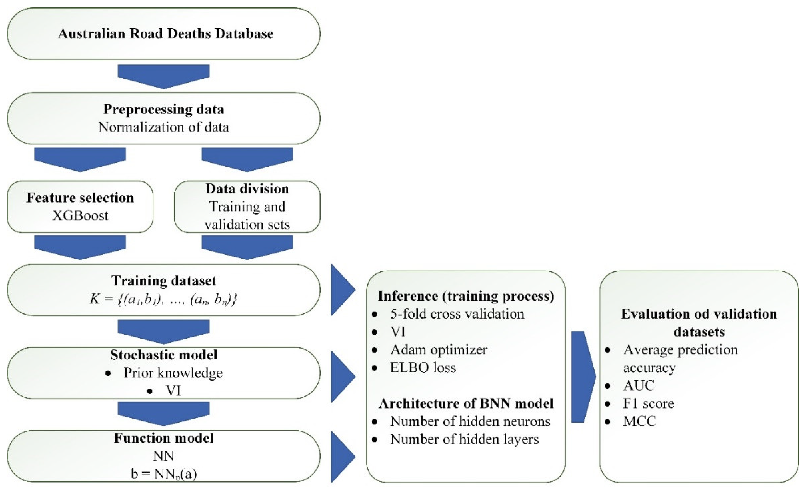
3. Methodology
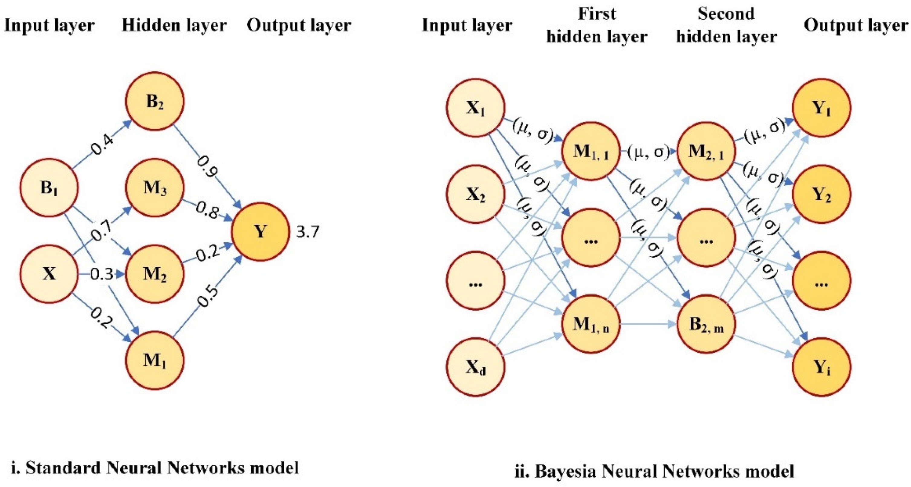
3.1. A Basic Understanding of the Bayesian Neural Network and Bayesian Inference
3.2. Bayesian Neural Network
3.3. Evaluation of Various Models’ Performances
- Average training accuracy (ATA): Prediction accuracy in this study’s binary class case is defined as the total number of correct forecasts over two classes divided by the total number of forecasts.
- Average F1-score: In the binary-class forecasting study, the average F1-score was employed to approximate criteria for each classification, and the average was calculated by estimating the number of correctly predicted occurrences.
- The area under the ROC curve (AUC): the area under the receiver operating characteristic curve (AUC) was utilised to estimate a scoring classifier at multiple cutoffs in this investigation. The AUC measures a model’s ability to distinguish between positive and negative classifications.
- Matthew’s correlation coefficient (MCC): The MCC was employed to assess the quality of binary classifications in this investigation. The MCC is a balanced measure that can be utilized even if the categories are of significantly distinct sizes, since it considers true and inaccurate positives and negatives. This criterion is a correlation coefficient that produces a number between -1 and +1 for actual and forecasted binary classes.
3.4. Dataset
- The order of nominal variables was rearranged, with the smallest category appearing first and the largest category appearing last.
- In continuous variables, missing values were substituted with the mean.
- The mode was used to substitute missing values in nominal variables.
- The median was utilized to substitute missing values in ordinal variables.
- The target variable (road user) was initially nominal, and its values included driver, motorcycle pillion passenger, motorcycle rider, passenger, pedal cyclist, pedestrian. The road user was transformed into a binary variable. This new variable included two classes: non-pedestrian death and pedestrian death.
4. Results and Discussions
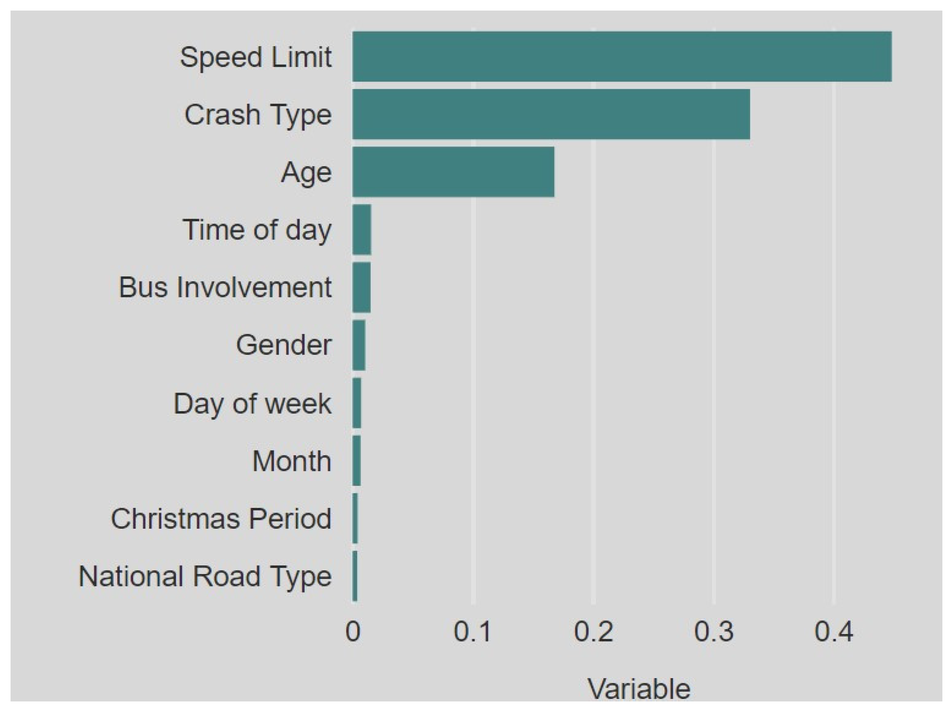
4.1. Determination of Significant Variables
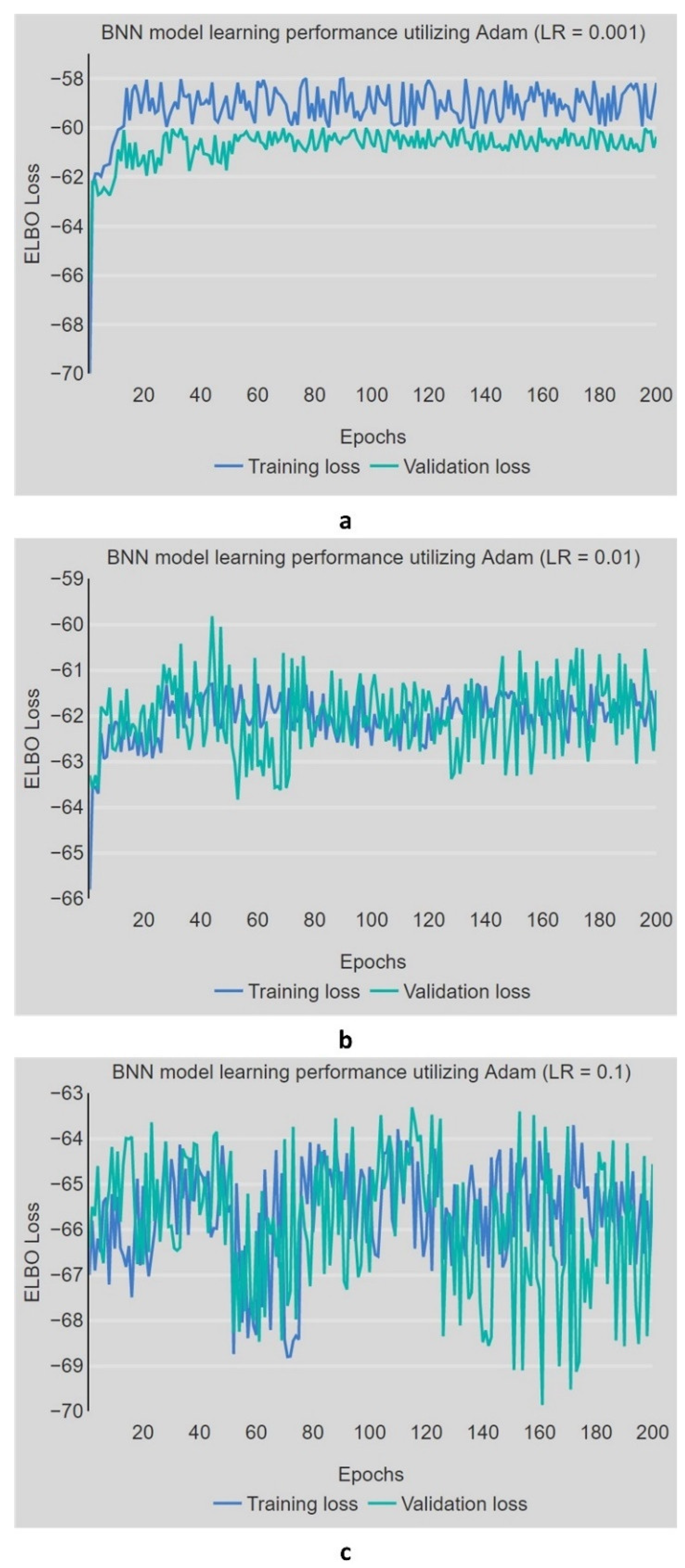
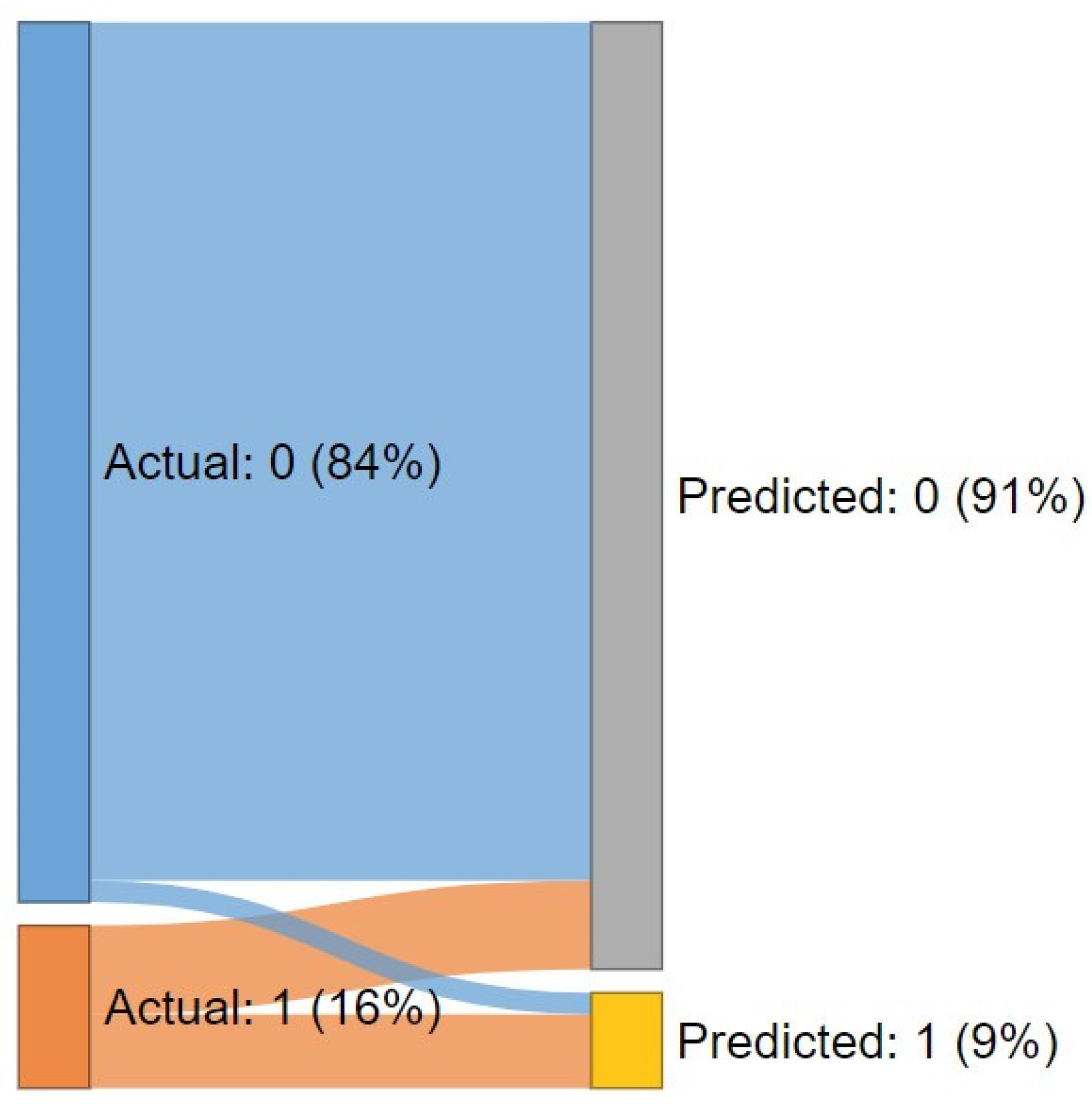
4.2. Development and Performance Assessment of the BNN Model
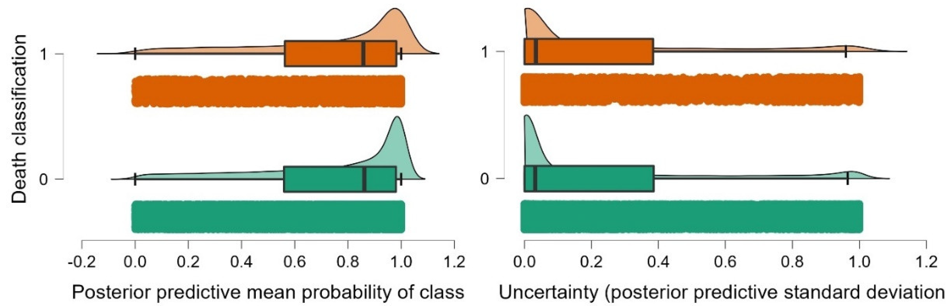
4.3. Quantification of Ambiguity in the Forecast and Classifying Probability
4.4. Variable Significance
4.5. Comparison of BNN Modes with Other ML Models
4.6. Limitations and Future Enhancements
5. Conclusions
- The BNN model, which consists of three hidden neuron layers with sixteen hidden nodes in the first layer, provided the best training accuracy of 0.894. Its posterior predictive probabilities are in the great probability range, and the predictive ambiguity is tightly concentrated in the 0–0.1 range.
- BNN model outperformed RF, BN, and NN models.
- Personal characteristics and time and occasion factor groups are clearly essential, greatly boosting the performance of the model if they are used as inputs.
- Individually, the most important parameters in PDRC prediction were the speed limit, collision type, and age.
Author Contributions
Funding
Acknowledgments
Conflicts of Interest
References
- Australian Transport Council (ATC). National Road Safety Strategy 2011–2020; Australian Transport Council: Canberra, Australia, 2011.
- Department of Infrastructure Regional Development and Cities. Australian Road Deaths Database. 2021. Available online: https://www.bitre.gov.au/statistics/safety/fatal_road_crash_database (accessed on 13 November 2021).
- Bureau of Infrastructure, Transport and Regional Economics. Road Trauma Involving Heavy Vehicles 2018 Crash Statistical Summary; BITRE: Canberra, Australia, 2020.
- Zegeer, C.V.; Bushell, M. Pedestrian crash trends and potential countermeasures from around the world. Accid. Anal. Prev. 2012, 44, 3–11. [Google Scholar] [CrossRef] [PubMed]
- Anderson, R.; Ponte, G.; Doecke, S. A Survey of Bullbar Prevalence at Pedestrian Crash Sites in Adelaide, South Australia; Centre for Automotive Safety Research: Adelaide, Australia, 2008. [Google Scholar]
- Samerei, S.A.; Aghabayk, K.; Shiwakoti, N.; Karimi, S. Modelling bus-pedestrian crash severity in the state of Victoria, Australia. Int. J. Inj. Control Saf. Promot. 2021, 28, 233–242. [Google Scholar] [CrossRef] [PubMed]
- Arnold, P.; Rosman, D.; Thornett, M. Pedestrian crash risk in Western Australia for both pedestrians and drivers. Road Transp. Res. 1992, 1, 60–75. [Google Scholar]
- Imprialou, M.; Quddus, M. Crash data quality for road safety research: Current state and future directions. Accid. Anal. Prev. 2019, 130, 84–90. [Google Scholar] [CrossRef] [Green Version]
- Mannering, F.L.; Bhat, C.R. Analytic methods in accident research: Methodological frontier and future directions. Anal. Methods Accid. Res. 2014, 1, 1–22. [Google Scholar] [CrossRef]
- Shaheed, M.S.; Gkritza, K. A latent class analysis of single-vehicle motorcycle crash severity outcomes. Anal. Methods Accid. Res. 2014, 2, 30–38. [Google Scholar] [CrossRef]
- Sun, M.; Sun, X.; Shan, D. Pedestrian crash analysis with latent class clustering method. Accid. Anal. Prev. 2019, 124, 50–57. [Google Scholar] [CrossRef]
- Aghaabbasi, M.; Shekari, Z.A.; Shah, M.Z.; Olakunle, O.; Armaghani, D.J.; Moeinaddini, M. Predicting the use frequency of ride-sourcing by off-campus university students through random forest and Bayesian network techniques. Transp. Res. Part A Policy Pract. 2020, 136, 262–281. [Google Scholar] [CrossRef]
- Qian, Y.; Aghaabbasi, M.; Ali, M.; Alqurashi, M.; Salah, B.; Zainol, R.; Moeinaddini, M.; Hussein, E.E. Classification of Imbalanced Travel Mode Choice to Work Data Using Adjustable SVM Model. Appl. Sci. 2021, 11, 11916. [Google Scholar] [CrossRef]
- Aghaabbasi, M.; Shah, M.Z.; Zainol, R. Investigating the Use of Active Transportation Modes Among University Employees Through an Advanced Decision Tree Algorithm. Civ. Sustain. Urban Eng. 2021, 1, 26–49. [Google Scholar] [CrossRef]
- Ali, M.; de Azevedo, A.R.G.; Marvila, M.T.; Khan, M.I.; Memon, A.M.; Masood, F.; Almahbashi, N.M.Y.; Shad, M.K.; Khan, M.A.; Fediuk, R.; et al. The Influence of COVID-19-Induced Daily Activities on Health Parameters—A Case Study in Malaysia. Sustainability 2021, 13, 7465. [Google Scholar] [CrossRef]
- Ali, M.; Dharmowijoyo, D.B.; Harahap, I.S.; Puri, A.; Tanjung, L.E. Travel behaviour and health: Interaction of Activity-Travel Pattern, Travel Parameter and Physical Intensity. Solid State Technol. 2020, 63, 4026–4039. [Google Scholar]
- Ali, M.; Dharmowijoyo, D.B.E.; de Azevedo, A.R.G.; Fediuk, R.; Ahmad, H.; Salah, B. Time-Use and Spatio-Temporal Variables Influence on Physical Activity Intensity, Physical and Social Health of Travelers. Sustainability 2021, 13, 12226. [Google Scholar] [CrossRef]
- Chen, Y.; Aghaabbasi, M.; Ali, M.; Anciferov, S.; Sabitov, L.; Chebotarev, S.; Nabiullina, K.; Sychev, E.; Fediuk, R.; Zainol, R. Hybrid Bayesian Network Models to Investigate the Impact of Built Environment Experience before Adulthood on Students’ Tolerable Travel Time to Campus: Towards Sustainable Commute Behavior. Sustainability 2022, 14, 325. [Google Scholar] [CrossRef]
- Xie, Y.; Lord, D.; Zhang, Y. Predicting motor vehicle collisions using Bayesian neural network models: An empirical analysis. Accid. Anal. Prev. 2007, 39, 922–933. [Google Scholar] [CrossRef]
- Ali, M.; Abbas, S.; Salah, B.; Akhter, J.; Saleem, W.; Haruna, S.; Room, S.; Abdulkadir, I. Investigating Optimal Confinement Behaviour of Low-Strength Concrete through Quantitative and Analytical Approaches. Materials 2021, 14, 4675. [Google Scholar] [CrossRef] [PubMed]
- Ali, M.; Room, S.; Khan, M.I.; Masood, F.; Ali Memon, R.; Khan, R.; Memon, A.M. Assessment of local earthen bricks in perspective of physical and mechanical properties using Geographical Information System in Peshawar, Pakistan. Structures 2020, 28, 2549–2561. [Google Scholar] [CrossRef]
- De Azevedo, A.R.G.; Marvila, M.T.; Ali, M.; Khan, M.I.; Masood, F.; Vieira, C.M.F. Effect of the addition and processing of glass polishing waste on the durability of geopolymeric mortars. Case Stud. Constr. Mater. 2021, 15, e00662. [Google Scholar] [CrossRef]
- Liu, T.; Liu, Y.; Liu, J.; Wang, L.; Xu, L.; Qiu, G.; Gao, H. A Bayesian learning based scheme for online dynamic security assessment and preventive control. IEEE Trans. Power Syst. 2020, 35, 4088–4099. [Google Scholar] [CrossRef]
- Marzban, C.; Witt, A. A Bayesian neural network for severe-hail size prediction. Weather Forecast. 2001, 16, 600–610. [Google Scholar] [CrossRef]
- Yan, D.; Zhou, Q.; Wang, J.; Zhang, N. Bayesian regularisation neural network based on artificial intelligence optimisation. Int. J. Prod. Res. 2017, 55, 2266–2287. [Google Scholar] [CrossRef]
- Zajac, S.S.; Ivan, J.N. Factors influencing injury severity of motor vehicle–crossing pedestrian crashes in rural Connecticut. Accid. Anal. Prev. 2003, 35, 369–379. [Google Scholar] [CrossRef]
- Rifaat, S.M.; Chin, H.C. Accident severity analysis using ordered probit model. J. Adv. Transp. 2007, 41, 91–114. [Google Scholar] [CrossRef]
- Obeng, K.; Rokonuzzaman, M. Pedestrian injury severity in automobile crashes. Open J. Saf. Sci. Technol. 2013, 3, 33341. [Google Scholar] [CrossRef] [Green Version]
- Kwigizile, V.; Sando, T.; Chimba, D. Inconsistencies of ordered and unordered probability models for pedestrian injury severity. Transp. Res. Rec. 2011, 2264, 110–118. [Google Scholar] [CrossRef]
- Yasmin, S.; Eluru, N. Evaluating alternate discrete outcome frameworks for modeling crash injury severity. Accid. Anal. Prev. 2013, 59, 506–521. [Google Scholar] [CrossRef]
- Sze, N.-N.; Wong, S. Diagnostic analysis of the logistic model for pedestrian injury severity in traffic crashes. Accid. Anal. Prev. 2007, 39, 1267–1278. [Google Scholar] [CrossRef]
- Kim, S.; Ulfarsson, G.F. Traffic safety in an aging society: Analysis of older pedestrian crashes. J. Transp. Saf. Secur. 2019, 11, 323–332. [Google Scholar] [CrossRef]
- Ulfarsson, G.F.; Kim, S.; Booth, K.M. Analyzing fault in pedestrian–motor vehicle crashes in North Carolina. Accid. Anal. Prev. 2010, 42, 1805–1813. [Google Scholar] [CrossRef]
- Tay, R.; Choi, J.; Kattan, L.; Khan, A. A multinomial logit model of pedestrian–vehicle crash severity. Int. J. Sustain. Transp. 2011, 5, 233–249. [Google Scholar] [CrossRef]
- Zhou, Z.-P.; Liu, Y.-S.; Wang, W.; Zhang, Y. Multinomial logit model of pedestrian crossing behaviors at signalized intersections. Discret. Dyn. Nat. Soc. 2013, 2013, 172726. [Google Scholar] [CrossRef]
- Chen, Z.; Fan, W. Modeling pedestrian injury severity in pedestrian-vehicle crashes in rural and urban areas: Mixed logit model approach. Transp. Res. Rec. 2019, 2673, 1023–1034. [Google Scholar] [CrossRef]
- Kim, J.-K.; Ulfarsson, G.F.; Shankar, V.N.; Mannering, F.L. A note on modeling pedestrian-injury severity in motor-vehicle crashes with the mixed logit model. Accid. Anal. Prev. 2010, 42, 1751–1758. [Google Scholar] [CrossRef]
- Haleem, K.; Alluri, P.; Gan, A. Analyzing pedestrian crash injury severity at signalized and non-signalized locations. Accid. Anal. Prev. 2015, 81, 14–23. [Google Scholar] [CrossRef]
- Tulu, G.S.; Washington, S.; Haque, M.M.; King, M.J. Injury severity of pedestrians involved in road traffic crashes in Addis Ababa, Ethiopia. J. Transp. Saf. Secur. 2017, 9, 47–66. [Google Scholar] [CrossRef]
- Rifaat, S.M.; Tay, R.; de Barros, A. Urban street pattern and pedestrian traffic safety. J. Urban Des. 2012, 17, 337–352. [Google Scholar] [CrossRef]
- Sasidharan, L.; Menéndez, M. Partial proportional odds model—An alternate choice for analyzing pedestrian crash injury severities. Accid. Anal. Prev. 2014, 72, 330–340. [Google Scholar] [CrossRef]
- Pour, A.T.; Moridpour, S.; Tay, R.; Rajabifard, A. A partial proportional odds model for pedestrian crashes at mid-blocks in Melbourne metropolitan area. MATEC Web Conf. 2016, 81, 02020. [Google Scholar] [CrossRef] [Green Version]
- Li, Y.; Fan, W.D. Modelling severity of pedestrian-injury in pedestrian-vehicle crashes with latent class clustering and partial proportional odds model: A case study of North Carolina. Accid. Anal. Prev. 2019, 131, 284–296. [Google Scholar] [CrossRef]
- Li, Y.; Fan, W. Pedestrian injury severities in pedestrian-vehicle crashes and the partial proportional odds logit model: Accounting for age difference. Transp. Res. Rec. 2019, 2673, 731–746. [Google Scholar] [CrossRef]
- Chang, L.-Y.; Chen, W.-C. Data mining of tree-based models to analyze freeway accident frequency. J. Saf. Res. 2005, 36, 365–375. [Google Scholar] [CrossRef]
- Gong, Y.; Abdel-Aty, M.; Cai, Q.; Rahman, M.S. A decentralized network level adaptive signal control algorithm by deep reinforcement learning. In Proceedings of the Transportation Research Board 98th Annual Meeting, Washington, DC, USA, 13–17 January 2019. [Google Scholar]
- Zhu, S.Y. Analyse vehicle-pedestrian crash severity at intersection with data mining techniques. Int. J. Crashworthiness 2021, 1–9. [Google Scholar] [CrossRef]
- Mackay, D.J.C. Bayesian Methods for Adaptive Models. Ph.D. Thesis, California Institute of Technology, Pasadena, CA, USA, 1992. [Google Scholar]
- Neal, R.M. Bayesian Learning for Neural Networks; Springer Science & Business Media: Berlin/Heidelberg, Germany, 2012; Volume 118. [Google Scholar]
- Liang, F. Bayesian neural networks for nonlinear time series forecasting. Stat. Comput. 2005, 15, 13–29. [Google Scholar] [CrossRef]
- Riviere, C.; Lauret, P.; Ramsamy, J.M.; Page, Y. A Bayesian neural network approach to estimating the energy equivalent speed. Accid. Anal. Prev. 2006, 38, 248–259. [Google Scholar] [CrossRef]
- Pour, A.T.; Moridpour, S.; Rajabifard, A.; Tay, R. Spatial and temporal distribution of pedestrian crashes in Melbourne metropolitan area. Road Transp. Res. 2017, 26, 4–20. [Google Scholar]
- Ding, C.; Chen, P.; Jiao, J.F. Non-linear effects of the built environment on automobile-involved pedestrian crash frequency: A machine learning approach. Accid. Anal. Prev. 2018, 112, 116–126. [Google Scholar] [CrossRef]
- Mokhtarimousavi, S. A Time of Day Analysis of Pedestrian-Involved Crashes in California: Investigation of Injury Severity, a Logistic Regression and Machine Learning Approach Using HSIS Data. ITE J.-Inst. Transp. Eng. 2019, 89, 25–33. [Google Scholar]
- Das, S.; Le, M.; Dai, B.Y. Application of machine learning tools in classifying pedestrian crash types: A case study. Transp. Saf. Environ. 2020, 2, 106–119. [Google Scholar] [CrossRef]
- Rahimi, A.; Azimi, G.; Asgari, H.; Jin, X. Injury Severity of Pedestrian and Bicyclist Crashes Involving Large Trucks. In Proceedings of the ASCE International Conference on Transportation and Development (ASCE ICTD), Seattle, WA, USA, 26–29 May 2020; pp. 110–122. [Google Scholar]
- Guo, M.; Yuan, Z.; Janson, B.; Peng, Y.; Yang, Y.; Wang, W. Older pedestrian traffic crashes severity analysis based on an emerging machine learning XGBoost. Sustainability 2021, 13, 926. [Google Scholar] [CrossRef]
- Saha, D.; Dumbaugh, E. Use of a model-based gradient boosting framework to assess spatial and non-linear effects of variables on pedestrian crash frequency at macro-level. J. Transp. Saf. Secur. 2021, 13, 32. [Google Scholar] [CrossRef]
- Wang, H.; Yeung, D.-Y. Towards Bayesian deep learning: A framework and some existing methods. IEEE Trans. Knowl. Data Eng. 2016, 28, 3395–3408. [Google Scholar] [CrossRef] [Green Version]
- Blei, D.M.; Kucukelbir, A.; McAuliffe, J.D. Variational inference: A review for statisticians. J. Am. Stat. Assoc. 2017, 112, 859–877. [Google Scholar] [CrossRef] [Green Version]
- Wu, S.; Yuan, Q.; Yan, Z.; Xu, Q. Analyzing Accident Injury Severity via an Extreme Gradient Boosting (XGBoost) Model. J. Adv. Transp. 2021, 2021, 3771640. [Google Scholar] [CrossRef]
- Chen, T.; Guestrin, C. Xgboost: A scalable tree boosting system. In Proceedings of the 22nd ACM SIGKDD International Conference on Knowledge Discovery and Data Mining, San Francisco, CA, USA, 13–17 August 2016; pp. 785–794. [Google Scholar]
- Onieva-García, M.Á.; Martínez-Ruiz, V.; Lardelli-Claret, P.; Jiménez-Moleón, J.J.; Amezcua-Prieto, C.; de Dios Luna-del-Castillo, J.; Jiménez-Mejías, E. Gender and age differences in components of traffic-related pedestrian death rates: Exposure, risk of crash and fatality rate. Inj. Epidemiol. 2016, 3, 14. [Google Scholar] [CrossRef] [Green Version]
- Toran Pour, A.; Moridpour, S.; Tay, R.; Rajabifard, A. Influence of pedestrian age and gender on spatial and temporal distribution of pedestrian crashes. Traffic Inj. Prev. 2018, 19, 81–87. [Google Scholar] [CrossRef]
- Park, S.; Ko, D. Investigating the Factors Influencing Pedestrian–Vehicle Crashes by Age Group in Seoul, South Korea: A Hierarchical Model. Sustainability 2020, 12, 4239. [Google Scholar] [CrossRef]
- Kim, J.-K.; Ulfarsson, G.F.; Shankar, V.N.; Kim, S. Age and pedestrian injury severity in motor-vehicle crashes: A heteroskedastic logit analysis. Accid. Anal. Prev. 2008, 40, 1695–1702. [Google Scholar] [CrossRef]
- Park, H.-C.; Joo, Y.-J.; Kho, S.-Y.; Kim, D.-K.; Park, B.-J. Injury severity of bus–pedestrian crashes in South Korea considering the effects of regional and company factors. Sustainability 2019, 11, 3169. [Google Scholar] [CrossRef] [Green Version]
- Li, P.; Abdel-Aty, M.; Yuan, J. Using bus critical driving events as surrogate safety measures for pedestrian and bicycle crashes based on GPS trajectory data. Accid. Anal. Prev. 2021, 150, 105924. [Google Scholar] [CrossRef]
- Sivasankaran, S.K.; Balasubramanian, V. Severity of Pedestrians in Pedestrian-Bus Crashes: An Investigation of Pedestrian, Driver and Environmental Characteristics Using Random Forest Approach. In Proceedings of the Congress of the International Ergonomics Association, Online, 13–18 June 2021; pp. 825–833. [Google Scholar]
- Breiman, L. Random forests. Mach. Learn. 2001, 45, 5–32. [Google Scholar] [CrossRef] [Green Version]
- Shawky, M.; Garib, A.; Al-Harthei, H. The impact of road and site characteristics on the crash-injury severity of pedestrian crashes. Adv. Transp. Stud. 2014, 1, 27–36. [Google Scholar]
- Zhai, X.; Huang, H.; Sze, N.; Song, Z.; Hon, K.K. Diagnostic analysis of the effects of weather condition on pedestrian crash severity. Accid. Anal. Prev. 2019, 122, 318–324. [Google Scholar] [CrossRef] [PubMed]
- Ukkusuri, S.; Miranda-Moreno, L.F.; Ramadurai, G.; Isa-Tavarez, J. The role of built environment on pedestrian crash frequency. Saf. Sci. 2012, 50, 1141–1151. [Google Scholar] [CrossRef]
- Jain, A.; Gupta, A.; Rastogi, R. Pedestrian crossing behaviour analysis at intersections. Int. J. Traffic Transp. Eng. 2014, 4, 103–116. [Google Scholar] [CrossRef] [Green Version]
- Kucerová, I.; Sulíková, B.; Polácková, K. Pedestrian accidents-actual trend in the Czech Republic. Trans. Transp. Sci. 2013, 6, 145. [Google Scholar] [CrossRef] [Green Version]
- Aarts, L.; Van Schagen, I. Driving speed and the risk of road crashes: A review. Accid. Anal. Prev. 2006, 38, 215–224. [Google Scholar] [CrossRef]
- Read, D.J. Open speeds on Northern Territory roads: Not so fast. Med. J. Aust. 2015, 203, 14–15. [Google Scholar] [CrossRef] [Green Version]
- Oxley, J.; Whelan, M. It cannot be all about safety: The benefits of prolonged mobility. Traffic Inj. Prev. 2008, 9, 367–378. [Google Scholar] [CrossRef]


| Variable and Sub-variable | Description | Value | Mean/Mode |
|---|---|---|---|
| Individual characteristics (IC) | |||
| Age | Age of the individual who was killed (years) | 1–101 | 39.662 |
| Gender | Person’s sex | Female, male | Male |
| Time and occasions (TO) | |||
| Month | Month of crash | 1–12 | 12 |
| Day of week | Specifies whether the crash happened on a weekday or on a weekend. | Weekend; weekday | Weekday |
| Time of day | Specifies whether the crash happened during the day or at night. | Day, Night | Day |
| Christmas Period | Specifies whether the crash happened in the 12 days starting on 23 December. | Yes, no | No |
| Easter Period | Specifies whether the crash happened within the five days leading up to Good Friday. | Yes, no | No |
| Road characteristics (RC) | |||
| Speed limit | The designated speed limit at the location of the crash. | 10–130 km | 82.10 |
| National Road Type | Access Road, Arterial Road, Collector Road, Local Road, National or State Highway, Pedestrian Thoroughfare, Sub-arterial Road | National or State Highway | |
| Crash attributes (CA) | |||
| Crash Type | If a pedestrian was died in a collision, it is marked as a pedestrian crash; else, the vehicles engaged is recorded. | Multiple, single | Single |
| Bus involvement | Shows that a bus was involved in the accident. | Yes, no | No |
| Heavy Rigid Truck Involvement | Shows that a heavy rigid truck was involved in the collision. | Yes, no | No |
| Road User (target variable) | Road user type of killed person. | Non-pedestrian, pedestrian | Non-pedestrian |
| NS | HL | ATA | Sensitivity | Specificity | Precision | NPV | FPR | FDR | FNR | F1 Score | AUC | MCC |
|---|---|---|---|---|---|---|---|---|---|---|---|---|
| NS1 | 1 | 0.802 | 0.940 | 0.421 | 0.817 | 0.721 | 0.578 | 0.182 | 0.059 | 0.874 | 0.808 | 0.442 |
| NS2 | 1 | 0.834 | 0.844 | 0.171 | 0.986 | 0.015 | 0.828 | 0.013 | 0.155 | 0.909 | 0.748 | 0.005 |
| NS3 | 1 | 0.879 | 0.890 | 0.747 | 0.974 | 0.345 | 0.252 | 0.021 | 0.110 | 0.932 | 0.776 | 0.454 |
| NS4 | 1 | 0.887 | 0.900 | 0.752 | 0.974 | 0.413 | 0.247 | 0.025 | 0.100 | 0.939 | 0.780 | 0.503 |
| NS5 | 2 | 0.607 | 0.967 | 0.271 | 0.553 | 0.900 | 0.728 | 0.446 | 0.032 | 0.704 | 0.811 | 0.329 |
| NS6 | 2 | 0.570 | 0.972 | 0.256 | 0.504 | 0.922 | 0.743 | 0.4951 | 0.027 | 0.664 | 0.811 | 0.312 |
| NS7 | 2 | 0.670 | 0.9605 | 0.303 | 0.636 | 0.858 | 0.696 | 0.363 | 0.039 | 0.765 | 0.804 | 0.361 |
| NS8 | 2 | 0.767 | 0.947 | 0.379 | 0.766 | 0.771 | 0.620 | 0.233 | 0.052 | 0.847 | 0.796 | 0.419 |
| NS9 | 2 | 0.784 | 0.945 | 0.399 | 0.791 | 0.750 | 0.600 | 0.208 | 0.055 | 0.861 | 0.822 | 0.432 |
| NS10 | 3 | 0.867 | 0.879 | 0.687 | 0.976 | 0.274 | 0.313 | 0.023 | 0.120 | 0.925 | 0.824 | 0.377 |
| NS11 | 3 | 0.894 | 0.906 | 0.774 | 0.975 | 0.453 | 0.225 | 0.0245 | 0.093 | 0.939 | 0.844 | 0.540 |
| NS12 | 3 | 0.792 | 0.928 | 0.399 | 0.816 | 0.661 | 0.600 | 0.183 | 0.071 | 0.868 | 0.788 | 0.396 |
| NS13 | 3 | 0.781 | 0.944 | 0.394 | 0.786 | 0.750 | 0.605 | 0.213 | 0.055 | 0.858 | 0.734 | 0.426 |
| NS14 | 3 | 0.717 | 0.936 | 0.334 | 0.711 | 0.750 | 0.665 | 0.289 | 0.063 | 0.808 | 0.719 | 0.353 |
| NS15 | 3 | 0.707 | 0.949 | 0.334 | 0.687 | 0.811 | 0.665 | 0.312 | 0.050 | 0.797 | 0.717 | 0.376 |
| NS16 | 3 | 0.668 | 0.946 | 0.304 | 0.640 | 0.811 | 0.696 | 0.359 | 0.053 | 0.764 | 0.719 | 0.336 |
| Arrangement | Combination of Variables | ATA | F1 Score | AUC | MMC |
|---|---|---|---|---|---|
| ARR1 | IC + TO | 0.845 | 0.915 | 0.591 | 0.1375 |
| ARR2 | IC + RC | 0.855 | 0.918 | 0.698 | 0.324 |
| ARR3 | IC + CA | 0.858 | 0.920 | 0.761 | 0.317 |
| ARR4 | IC + TO + RC | 0.860 | 0.921 | 0.754 | 0.3527 |
| ARR5 | IC + TO + CA | 0.863 | 0.923 | 0.762 | 0.361 |
| ARR6 | IC + RC + CA | 0.890 | 0.937 | 0.788 | 0.526 |
| ARR7 | IC + TO + RC + CA | 0.894 | 0.939 | 0.844 | 0.540 |
| ARR8 | TO + RC | 0.844 | 0.915 | 0.500 | 0 |
| ARR9 | TO + CA | 0.846 | 0.916 | 0.695 | 0.113 |
| ARR10 | TO + RC + CA | 0.866 | 0.924 | 0.774 | 0.387 |
| ARR11 | RC + CA | 0.847 | 0.916 | 0.762 | 0.127 |
| Model | ATA | F1 Score | AUC | MMC |
|---|---|---|---|---|
| BNN | 0.89 | 0.94 | 0.84 | 0.54 |
| RF | 0.87 | 0.92 | 0.79 | 0.60 |
| BN | 0.85 | 0.91 | 0.80 | 0.36 |
| NN | 0.84 | 0.91 | 0.53 | 0.07 |
Publisher’s Note: MDPI stays neutral with regard to jurisdictional claims in published maps and institutional affiliations. |
© 2022 by the authors. Licensee MDPI, Basel, Switzerland. This article is an open access article distributed under the terms and conditions of the Creative Commons Attribution (CC BY) license (https://creativecommons.org/licenses/by/4.0/).
Share and Cite
Tao, W.; Aghaabbasi, M.; Ali, M.; Almaliki, A.H.; Zainol, R.; Almaliki, A.A.; Hussein, E.E. An Advanced Machine Learning Approach to Predicting Pedestrian Fatality Caused by Road Crashes: A Step toward Sustainable Pedestrian Safety. Sustainability 2022, 14, 2436. https://doi.org/10.3390/su14042436
Tao W, Aghaabbasi M, Ali M, Almaliki AH, Zainol R, Almaliki AA, Hussein EE. An Advanced Machine Learning Approach to Predicting Pedestrian Fatality Caused by Road Crashes: A Step toward Sustainable Pedestrian Safety. Sustainability. 2022; 14(4):2436. https://doi.org/10.3390/su14042436
Chicago/Turabian StyleTao, Wenlong, Mahdi Aghaabbasi, Mujahid Ali, Abdulrazak H. Almaliki, Rosilawati Zainol, Abdulrhman A. Almaliki, and Enas E. Hussein. 2022. "An Advanced Machine Learning Approach to Predicting Pedestrian Fatality Caused by Road Crashes: A Step toward Sustainable Pedestrian Safety" Sustainability 14, no. 4: 2436. https://doi.org/10.3390/su14042436