Predicting Model for Air Transport Demand under Uncertainties Based on Particle Filter

Abstract

The outbreak of the COVID-19 has brought about huge economic loss and civil aviation industries all over the world have suffered severe damage. An effective method is urgently needed to accurately predict air-transport demand under the influences of such accidental factors. This paper proposes a novel predicting framework for the air-transport demand considering the uncertainties caused by accidental factors including regional wars, climatic anomalies, and virus outbreaks. By employing a seasonal autoregressive integrated moving average (sARIMA) model as the basic model, a particle filter (PF)-based sARIMA-pf model is proposed. The applicability of adapting the high-order sARIMA model as the state transition model in a PF framework is shown and proven to be effective. The proposed method has the advantage of coping with short-term prediction with known uncertainties. By conducting case studies on the prediction of air passenger traffic volume in China, the sARIMA-pf model showed better performance than the sARIMA model and improved the accuracy by 49.29% and 44.96% under the conventional and pandemic scenarios, respectively, when using the root mean square error (RMSE) as the indicator.

1. Introduction

The COVID-19 pandemic has had a huge impact on the world economy, and especially on the civil aviation industry. According to the International Air Transport Association (IATA), the number of air passengers around the world decreased by 50% in 2021 compared to before COVID-19 and nearly USD 200 billion was lost in the past two years [1]. Air-transport demand is an important foundation on which airlines make flight schedules and airports make ground-support schemes. Facing the uncertainties caused by more and more accidental factors such as regional wars, climatic anomalies, and virus outbreaks, pursuing more dependable prediction methods to forecast air-transport demand inevitably becomes a central challenge for the civil aviation industry [2].

Air-transport-demand forecasting has been the focus of much research over recent decades. Prediction methods can be generally divided in to two categories: data-driven methods and model-based methods [3]. The traditional data-driven methods use historical data to fit the existing mathematical relationships such as linear and non-linear relationships, and the prediction results are obtained by extending the fitted methods to future time points. This method has been widely used in the engineering practice [4]. In fact, in most cases, the development of the air-transport demand can hardly be regarded as a linear or non-linear trend, instead, owing to holiday and fare factors, it should be regarded as a stochastic process with periodicity. The model-based methods try to model the stochastic process as a more complex relationship, as well as consider the influences of associated factors. One of the typical model-based methods is the autoregressive moving average (ARMA) model proposed by Box and Jenkins [5]. This model is further developed into the autoregressive integrated moving average (ARIMA) model and the seasonal ARIMA (sARIMA) model [6] to deal with the non-stationary data problem. Alberto and Postorino [7] conducted a test of ARIMA models on the Reggio Calabria airport and the test results showed that the models could predict the trend of the passenger throughput with a satisfactory result. Since air-transport demand shows periodic variations, sARIMA models have receiving wider attention than the other time-series models. Tsui et al. [8] forecasted Hong Kong airport’s passenger throughput with the sARIMA model and the multivariate ARIMA model (ARIMAX), and both models predicted a steady growth in future airport passenger traffic in Hong Kong.

Accidental factors make short-term air-transport demand change rapidly, as reported by IATA. Barczak et al. [9] estimated the differences between the demand that was observed during the pandemic and the demand that was forecast based on the pre-pandemic trend. The results showed that all the tested models failed when COVID-19 occurred, although all the tested models performed well ignoring the occurrence of the pandemic. The traditional models failed to describe the influences of the accidental factors because the models were established using only endogenous variables, but the accidental factors should be regarded as external variables for the air-transport-demand process. In other words, facing sudden uncertainty, the ARIMA-like models are conducted without incorporating more uncertain information.

Considering that the uncertainties caused by short-term external factors are difficult to model, two technological paths are getting increasing attention. One of the paths is a machine-learning method. Zhu et al. [10] proposed a novel deep-learning model framework to predict the airport throughput during the pandemic and their method showed better performance than baselines methods in departure-throughput predictions. As well as methods based on the neural networks, support vector machine methods [11,12] and K-nearest neighbor methods [12] are also commonly used machine learning models and often increase prediction accuracy. Although machine-learning methods have the advantage of predicting air-transport demand taking into account uncertainties caused by external variables such as a black box with the support of large number of data, it is still hard to interpret the relationships between the prediction results and the external variables. The methods are difficult to be utilize when there are less data to support them, and the scenarios with insufficient data are the situations faced by air-transport-demand forecasting. In the other path, hybrid models are applied by employing the information fusion ability of multiple methods. Jin et al. [13] tried to improve the prediction performance by proposing a new hybrid ensemble approach. By combining the kernel extreme learning machine with the ARMA model, their methods showed better robustness compared with the methods using single models. Wong et al. [14] combined the Markovian model with the Grey model and found that a fuzzy-Markovian model showed better performance on the observations with trends and intercepts. Normally, such hybrid methods show better performance under the certain circumstances, but the methods are also limited by the characteristics of the combined models. The method with universal applicability to different kinds of uncertainties is still under-researched.

Filtering methods [15,16] are commonly used to build the framework for solving various prediction problems with complex uncertainties [17,18], especially for the situations when there are less data. Filtering methods are able to make full use of the known information and are suitable to be employed for air-transport-demand forecasting. Typical filtering methods includes Kalman filter (KF), extended KF (EKF), and unscented KF (UKF) [19]. Since KF methods suppose that the noise signal should conform to Gaussian distribution, which is against the fact that to predict the air-transport demand, the accidental factors tend to follow arbitrary distributions, the particle filtering (PF) method with wider applicability including non-Gaussian and non-linear hypotheses was introduced [20]. Such kinds of models compromise the merits of data-driven models and have less demand in data quantity.

In this work, a novel universal framework for predicting air-transport demand with uncertainties is proposed. To overcome the disadvantages of the existing models, particle filtering is employed to establish the predicting framework and an sARIMA model is chosen as the basic model for common air-transport-demand forecasting. By using the framework, time-series models including ARIMA-based models can all be used as the basic model dealing with different forecasting scenarios. The proposed predicting method is called the sARIMA-pf method, and combines both time-series models and filtering methods to promote credibility with multiple uncertainties caused by accidental factors such as wars, epidemics, and extreme weather. One of the main contributions of this work is that the applicability of a high-order sARIMA used as the state transition model of the particle filter framework is shown and the effectiveness is proved. The rest of the paper is organized as follows: The framework for predicting the air-transport demand and the proposed sARIMA-pf technique is described in detail in Section 2. The situation of a high-order sARIMA model used as the state transition model in a PF framework is derived. In Section 3, the application of the method is verified by conducting the method on the volume of air passenger traffic of China and the comparisons with methods including sARIMA models under both step-by-step and target-time predicting scenarios are discussed. In Section 4, some conclusions and remarks are made.

2. Modeling Approaches

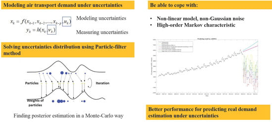
2.1. Particle-Filter Based Predicting Framework

The fluctuation of air traffic demand is influenced by multiple factors such as weather, substitution, fare changes, and epidemics. These external factors cause a difference between the real air-traffic demand and the volume of air-passenger traffic. In other words, the real air-traffic demand cannot be measured and can only be estimated by theory, and the volume of air-passenger traffic can be regarded as the observation of the real air-traffic demand. The proposed framework tries to establish a model to describe the theoretical development process and the observed volume of air passenger traffic.

Supposing that the real demand can be described as a sequence $x_{0:k}=\left\{x_0,x_1,\dots ,x_k\right\}$, where $x_k$ is the real demand at a certain time $k$. The corresponding observing value which is reflected by the volume of air passenger traffic or the airport throughput can be described as another sequence $y_{0:k}=\left\{y_0,y_1,\dots ,y_k\right\}$, where $y_k$ is the observed value at a certain time $k$. Then, the relationship between the real demand and the observation can be represented as

$$y_k=h(x_k,v_k)$$

(1)

where $h$ represents the measurement function and $v_k\in {\mathrm{R}}^{n_y}$ is used to describe the uncertainties of the observation process. $x_k\in {\mathrm{R}}^{n_x}$ is also called the state value of the observing system, $y_k\in {\mathrm{R}}^{n_y}$ is the measuring value of the system, $n_x$ is the dimension of the states, and $n_y$ is the dimension of the observations. It should be noted that the uncertainties of the observation process are mainly caused by statistical errors such as missing, repeated, and wrong records of the number of passengers for the prediction.

Meanwhile, the real demand is supposed to be follow the law of its own development. If the law of development is modelled, it can be described as

$$x_k=f(x_{k-1},u_k)$$

(2)

where $u_k\in {\mathrm{R}}^{n_x}$ is the independent, identically distributed uncertainties with known probability densities and $f$ represents the state transition function. It should be noted that the uncertainties of the development model include all the accidental factors.

For a practical prediction process, when an observation is obtained the number of passengers cannot be remeasured and the real demand cannot be obtained. Therefore, to promote the degree of credibility the process is translated into the process to find the posterior estimate of the real demand.

According to the Bayesian rule, the posterior estimation is common given by

$$p(x|y)=\frac{p(y|x)p(x)}{p(y)}=\frac{p(y|x)p(x)}{{\displaystyle {\displaystyle \int }p(y|x)p(x)\mathrm{d}x}}$$

(3)

where $p(x)$ and $p(y)$ are the probability distributions of state $x$ and observation $y$, and they should satisfy $p(y)>0$. Then, the problem for the prediction is to obtain the probability distributions $p(x_k|y_{0:k})$. $p(x_k|y_{0:k})$ is to estimate the value of $x_k$ using the observing information from the sequence $y_{0:k}=\left\{y_0,y_1,\dots ,y_k\right\}$. $p(x_0)=p(x_0|y_0)$ is supposed to be known distribution.

The prediction method can be regarded as the iteration of two main steps. The first step is the estimating step, in which the state value is estimated using the known information. The estimated value can be obtained by

$$p(x_k|y_{0:k})=\frac{p(y_k|x_k)p(x_k|y_{0:k-1})}{p(y_k|y_{1:k-1})}$$

(4)

The next step is the predicting step. The idea is to obtain the a priori estimate of the state. According to the Chapman–Kolmogorov formula, the a priori estimate can be obtained by

$$\begin{array}{c}p(x_k|y_{0:k-1})={\displaystyle \int p(x_k|x_{k-1},y_{0:k-1})p(x_{k-1}|y_{0:k-1})\mathrm{d}{x}_{k-1}}\\ ={\displaystyle \int p(x_k|x_{k-1})p(x_{k-1}|y_{0:k-1})\mathrm{d}{x}_{k-1}}\end{array}$$

(5)

where $p(x_k|x_{k-1})$ can be obtained by Equation (2). For the Equation (5), the value of $p(x_{k-1}|y_{0:k-1})$ is obtained by the last estimating step. Since the process is iteratively calculated, the estimating step can also be regarded as the updating step to calculate the value for predicting step.

In engineering practice, the posterior probability is rarely obtained using an analytical solution and to solve Equation (5), the particle filtering method is employed. Supposing that $\{x_{0:k}^i,i=1,2,\dots ,N\}$ is a set of particles, and $N$ is the number of the particles, a continuous probability distribution can be discretely described by the probability of occurrence of particles at each sampled value. The probability of particles’ occurrence can be obtained from the importance distribution $q(x_{0:k}|y_{0:k})$, and the importance weight for each particle can be calculated by

$${\omega }_k^i=\frac{p(x_{0:k}|y_{0:k})}{q(x_{0:k}|y_{0:k})}\propto {\omega }_{k-1}^i\frac{p(y_k|x_k^i)p(x_k^i|x_{k-1}^i)}{q(x_k^i|x_{k-1}^i,y_k)}$$

(6)

where ${\omega }_k^i$ is the weight of a particle at time $k$, and the posteriori distribution $p(x_k|y_{0:k})$ can be calculated by

$$p(x_k|y_{0:k})\approx {\displaystyle \sum _{i=1}^N{\omega }_k^i\mathsf{\delta }(x_k-x_k^i)}$$

(7)

where $\mathsf{\delta }$ is the Dirac function [21]. The weights of the particles are the probability of the uncertainties by the accidental factors.

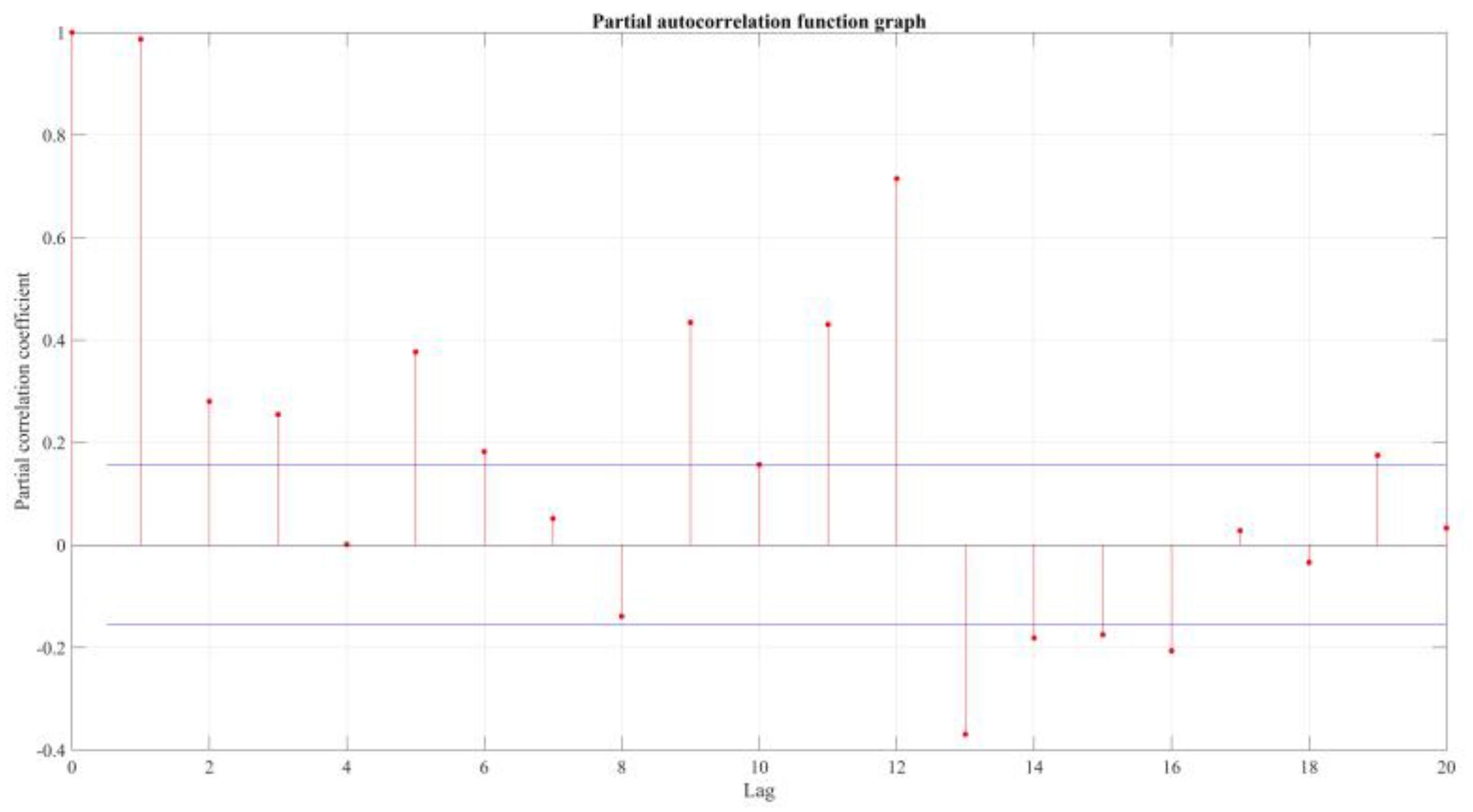
2.2. Seasonal Autoregressive Integrated Moving Average (sARIMA) Model

The ARIMA model is a type of time-series model, which is commonly used to model the air traffic demand. In this work, the sARIMA model is employed as part of the development model for the real-demand prediction as is described in Equation (2).

Since the sARIMA model is based on the ARIMA model, the ARIMA model is first introduced. When the differential order is set as 1, the model $\mathrm{ARMA}(p{}^{\prime },q)$ or $\mathrm{ARIMA}(p{}^{\prime },1,q)$ can be described by

$$x_k-{\varphi }_1{x}_{k-1}-{\varphi }_2{x}_{k-2}-\dots -{\varphi }_{p{}^{\prime }}{x}_{k-p{}^{\prime }}={\epsilon }_k+{\theta }_1{\epsilon }_{k-1}+{\theta }_2{\epsilon }_{k-2}+\dots +{\theta }_q{\epsilon }_{k-q},$$

(8)

where ${\epsilon }_k$ is the random error at time $k$, which is generally assumed to be independent, identically distributed variables sampled from a normal distribution with zero mean. ${\varphi }_i(i=1,2,\dots ,p{}^{\prime })$ and ${\theta }_j(j=1,2,\dots ,q)$ are model parameters. $p{}^{\prime }$ and $q$ are integers and often referred to as orders of the model. To introduce the model $\mathrm{ARIMA}(p,d,q)$, the lag operator $L$ should firstly be defined. For the sequence $x_{0:k}=\left\{x_0,x_1,\dots ,x_k\right\}$, the lag operator can be described as

$$L{x}_t=x_{t-1},t=2,\dots ,k.$$

(9)

Then the $\mathrm{ARIMA}(p{}^{\prime },1,q)$ can be written as

$$(1-{\displaystyle \sum _{i=1}^{p{}^{\prime }}{\varphi }_i{L}^i)x_i}=(1+{\displaystyle \sum _{i=1}^q{\theta }_i{L}^i){\epsilon }_k}$$

(10)

Assuming that the polynomial $(1-{\displaystyle \sum _{i=1}^p{\varphi }_i{L}^i)x_i}$ has a unit root of multiplicity $d$, then Equation (10) can be rewritten as

$$(1-{\displaystyle \sum _{i=1}^{p{}^{\prime }}{\varphi }_i{L}^i})=(1-{\displaystyle \sum _{i=1}^{p{}^{\prime }-d}{\phi }_i{L}^i}){(1-L)}^d$$

(11)

Substituting $p=p{}^{\prime }-d$ into Equation (11) yields

$$(1-{\displaystyle \sum _{i=1}^p{\phi }_i{L}^i}){(1-L)}^d{x}_k=(1+{\displaystyle \sum _{i=1}^q{\theta }_i{L}^i}){\epsilon }_k$$

(12)

which can be generalized as

$$(1-{\displaystyle \sum _{i=1}^p{\phi }_i{L}^i}){(1-L)}^d{x}_k=\delta +(1+{\displaystyle \sum _{i=1}^q{\theta }_i{L}^i}){\epsilon }_k$$

(13)

Based on the work of Box and Jenkins [5], a practical approach has been developed to build ARIMA models. The Box–Jenkins methodology includes three iterative steps of model identification, parameter estimation, and diagnostic checking. The basic idea of model identification is that if a time-series is generated from an ARIMA process, it should have some theoretical autocorrelation properties. By matching the empirical autocorrelation patterns with the theoretical ones, it is often possible to identify one or several potential models for the given time series [22]. This three-step model-building process is typically repeated several times until a satisfactory model is finally selected. The final selected model can then be used for prediction purposes.

sARIMA models are capable of modeling seasonal data compared with the non-seasonal ARIMA models. A seasonal ARIMA model is formed by including additional seasonal terms, which can be written as

$$\mathrm{ARIMA}(p,d,q){(P,D,Q)}_m$$

(14)

where $m$ is the number of observations per each time period and $P$, $D$, and $Q$ are the seasonal parameters of the model. The seasonal terms are multiplied by the non-seasonal terms to obtain the representation of sARIMA models. For details refer to [23].

2.3. The Proposed sARIMA-Pf Method

When the model whose order is $p$ as is given by Equation (8) is utilized as the development model of the real demand, Equation (2) should be rewritten as

$$x_k=f(x_{k-1},x_{k-2},\dots ,x_{k-p},u_k)$$

(15)

It should be noted that all the ARIMA-based models can be transformed to the form given by Equation (15).

Although the form of the model is different, the PF framework still takes hold and can be proven as follows. For the prediction step, the prior PDF of the state at time $k$ is

$$\begin{array}{cc}\hfill p(x_k|y_{0:k-1})& ={\displaystyle \int {\displaystyle \int \dots }}{\displaystyle \int p(x_k,x_{k-1},\dots ,x_{k-p}|y_{1:k-1})\mathrm{d}{x}_{k-1}\mathrm{d}{x}_{k-2}\dots \mathrm{d}{x}_{k-p}}\hfill \\ & ={\displaystyle \int {\displaystyle \int \dots }}{\displaystyle \int p(x_k|x_{k-1},x_{k-2},\dots ,x_{k-p},y_{0:k-1})p(x_{k-1}|y_{0:k-1})\dots p(x_{k-p}|y_{0:k-1})\mathrm{d}{x}_{k-1}\mathrm{d}{x}_{k-2}}\dots \mathrm{d}{x}_{k-p}\hfill \\ & ={\displaystyle \int {\displaystyle \int \dots }}{\displaystyle \int p(x_k|x_{k-1},x_{k-2},\dots ,x_{k-p})p(x_{k-1}|y_{0:k-1})\dots p(x_{k-p}|y_{0:k-p})\mathrm{d}{x}_{k-1}}\mathrm{d}{x}_{k-2}\dots \mathrm{d}{x}_{k-p}\hfill \end{array}$$

(16)

where $p(x_k|x_{k-1},x_{k-2},\dots ,x_{k-p})$ can be obtained by Equation (15), and $p(x_{k-p}|y_{0:k-p})$ is obtained by the update step in loop $k-p$. $p(x_0)=p(x_0|y_{0:0})$ is known previously.

For the update step, with a new observation $y_k$, the posterior probability distribution of the state can be calculated by Equations (5) and (6). Thus, the Bayesian solution is capable of being used in a high-order model.

Then, the proposed sARIMA-pf method can be described by the three main steps:

Step 1 Initialization: Given the historical observations $y_{0:k}=\left\{y_0,y_1,\dots ,y_k\right\}$, the sARIMA model $x_k=f_0(x_{k-1},x_{k-2},\dots ,x_{k-p_0},{\epsilon }_k)$ is firstly built. The number of particles $N$ is set. The particles and their weights are initialized as ${\{x_i^0=x_0+{\epsilon }_0,{\omega }_i^0=\frac{1}{N}\}}_{i=1}^N$, where ${\epsilon }_0$ is the probability distribution of the external accidental factors.

Step 2 Iteration: For the next time points $k+1$, when the new observation $y_{k+1}$ is obtained, calculating the posterior probability distribution of the state at the time point $k+1$ by using Equations (5) and (6) and updating the prior probability distribution of the state at point $k+2$ by using Equation (15). Normalizing the weight of each particle and conducting the resample according to the updating weights. Rebuilding the sARIMA model using the new observation sequence $y_{0:k+1}=\left\{y_0,y_1,\dots ,y_{k+1}\right\}$. For the next time points $k+2,k+3,\dots$, iterating the above process as needed, until it reaches the target time point.

Step 3 Prediction: The last a priori probability distribution of the state is the predicting result and the confidence interval concerning the uncertainties by the accidental factors can be obtained by counting the distribution of the particles.

2.4. Error Calculation

Mean square error (MSE) is commonly used to evaluate the performance of the prediction [24]. The model with lowest MSE is considered as the best model when using the MSE criterion. There are also other criteria such as root mean square error (RMSE), mean percentage error (MPE), and mean absolute error (MAE). By using such criteria, the performance of the different predicting methods can be compared and analyzed. Since the evaluating results of these criteria are nearly the same, the MSE and RMSE are employed in this paper to test the performance of the proposed method. The MSE and RMSE can be calculated by

$$\begin{array}{l}MSE=\frac{1}{m}{\displaystyle \sum _{i=1}^m{(y_i-{\widehat{y}}_i)}^2}\\ RMSE=\sqrt{MSE}\end{array}$$

(17)

where $m$ is the length of the predicting data, $y_i$ is the observed value, and ${\widehat{y}}_i$ is the predicted value.

3. Case Study

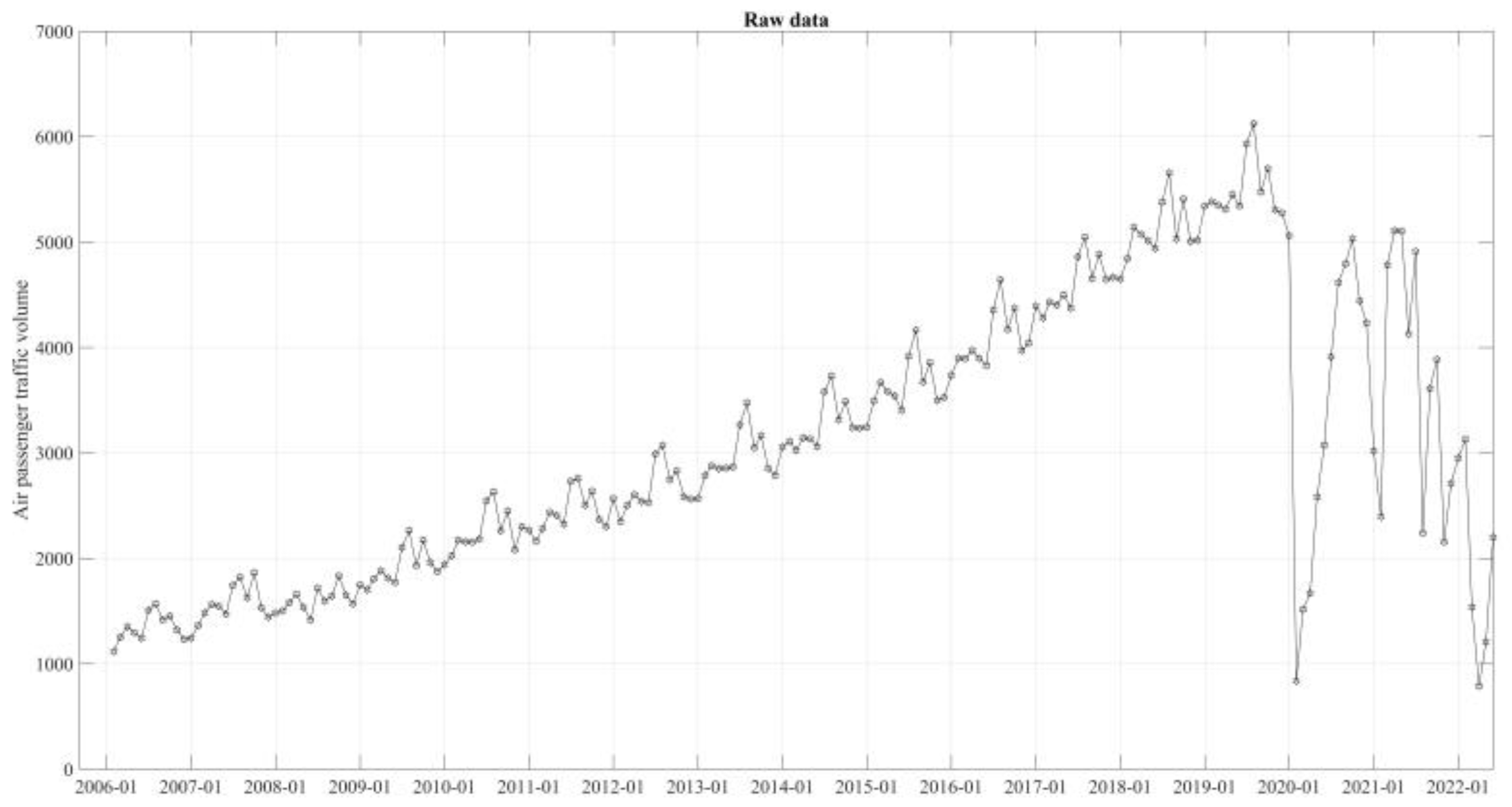
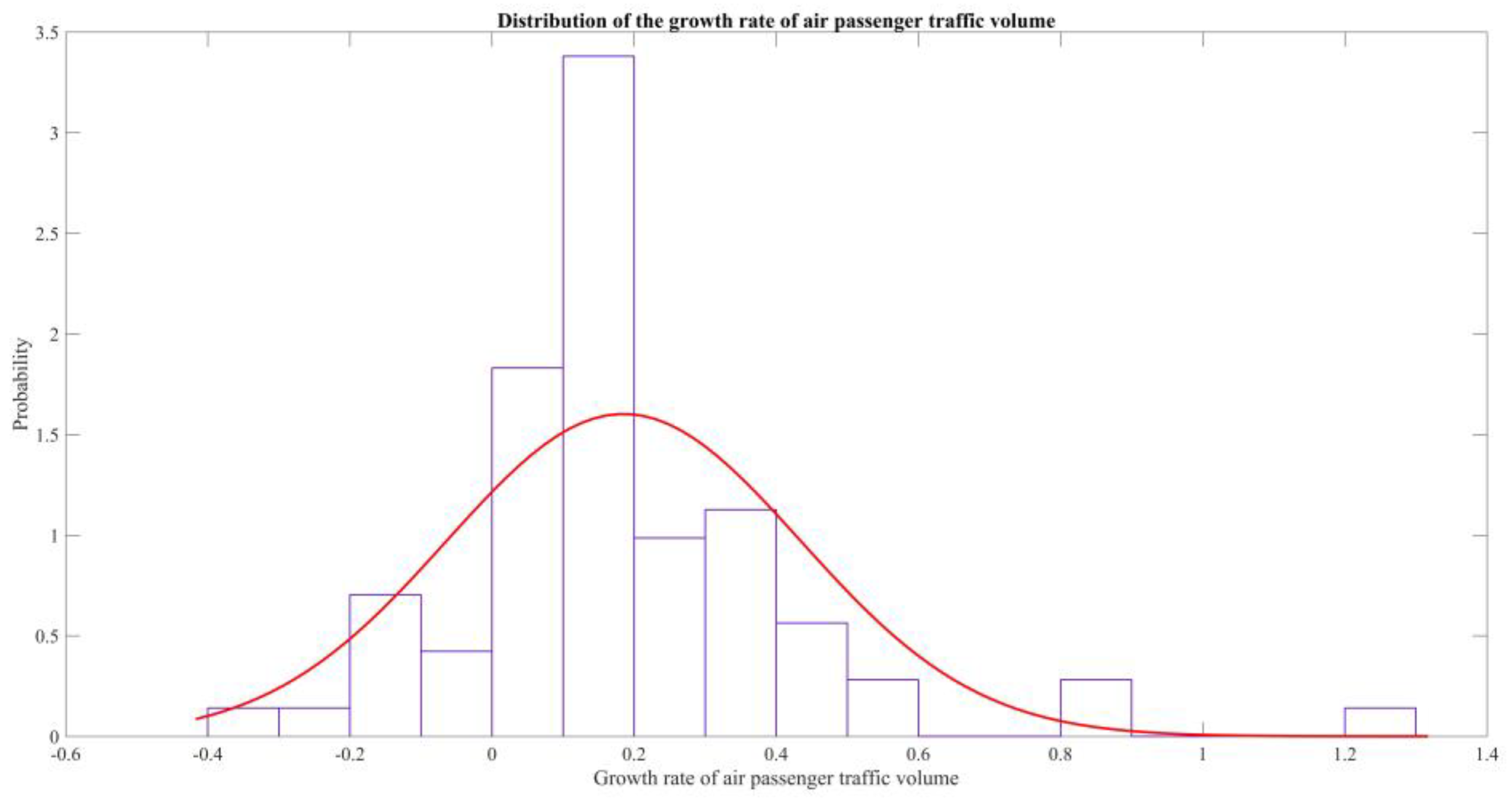
3.1. The Predicting Scenario and the Uncertainties Modeling

To verify the effectiveness of the proposed method, the air passenger traffic volume of China is employed to represent the air-transport demand in China. The air passenger traffic volume can be obtained from Civil Aviation Administration of China (CAAC, http://www.caac.gov.cn/en/SY/ (accessed on 27 October 2022)). As shown in Figure 1, the monthly air passenger traffic volume data from February 2006 to June 2022 were utilized to fit the model and test the results.

Two predicting scenarios were selected to test the performance of the proposed method. One of scenarios is regarded as the conventional scenario to predict the air passenger traffic volume before the outbreak of COVID-19. The other one is to predict the air passenger traffic volume under the COVID-19 pandemic. For the conventional scenario, the sARIMA method is usually believed to be one of the most accurate methods, hence, sARIMA was used for comparison. For the pandemic scenario, considering the sARIMA method may failed for long-term prediction, the step-by-step prediction was conducted for comparison.

Theoretically, with sufficient statistics, all kinds of known uncertainties can be modeled as a certain distribution. For single airports or airlines, the uncertainties may come from weather, economics, and so on. Geological disasters, changing weather, and economic activity usually happen regionally and only lead to limited impact on the air passenger traffic volume, which can be proved by the small difference in 2008 when the Wenchuan earthquake occurred and the Olympic games were held in Beijing, as shown in Figure 1. Even in 2003, when SARS-CoV was widely spread, it took only three months for the air passenger traffic volume of China to recover to the pre-pandemic levels. To simplify the fusion of different distributions and considering all the known and unknown uncertainties in this case, the growth rate of air passenger traffic volume was utilized as the indicator. It should be noted that the chosen indicator may represent the combined effect of both interior and external accidental factors, and it can be replaced by other distributions of uncertainties. The distribution of the growth rate of the air passenger traffic volume is shown in Figure 2. The distribution can be fitted as the Gaussian distribution N~(0.185, 0.249) and the probability of each value can be calculated by

$$prob=\frac{1}{\sqrt{2\ast pi\ast 0.249}}\ast e^{-\frac{1}{2}(\frac{{(x-0.185)}^2}{0.249})}.$$

(18)

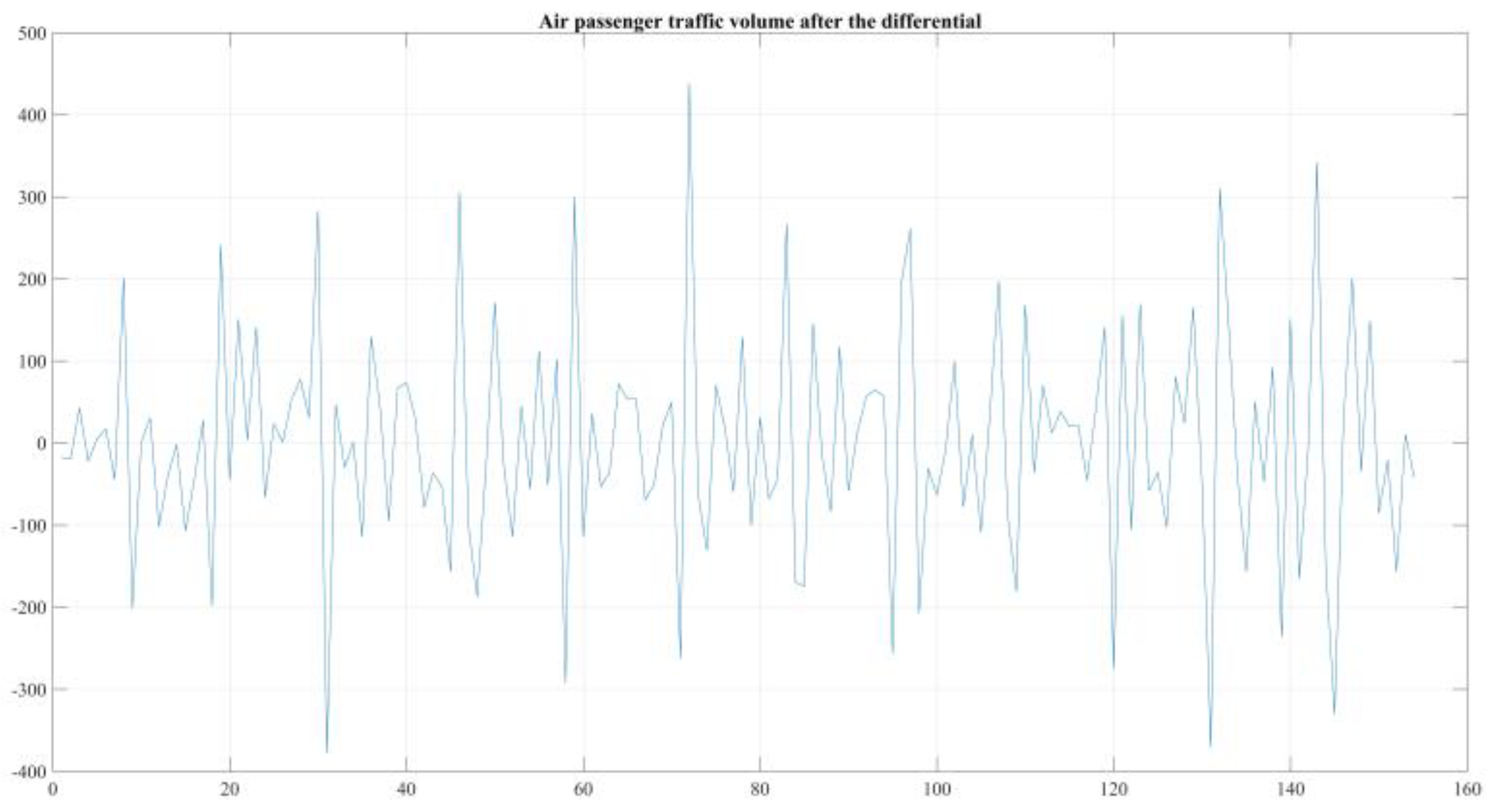
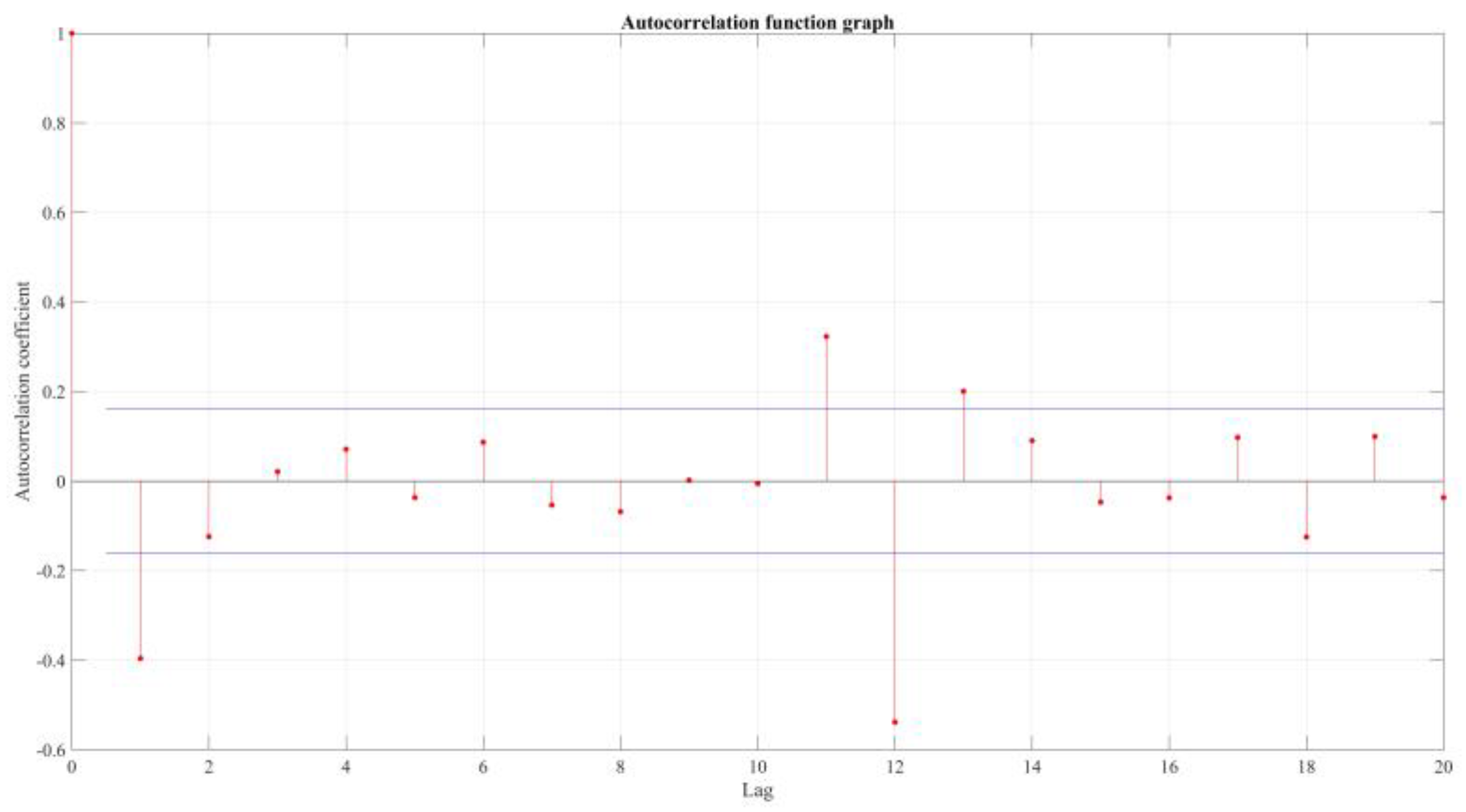
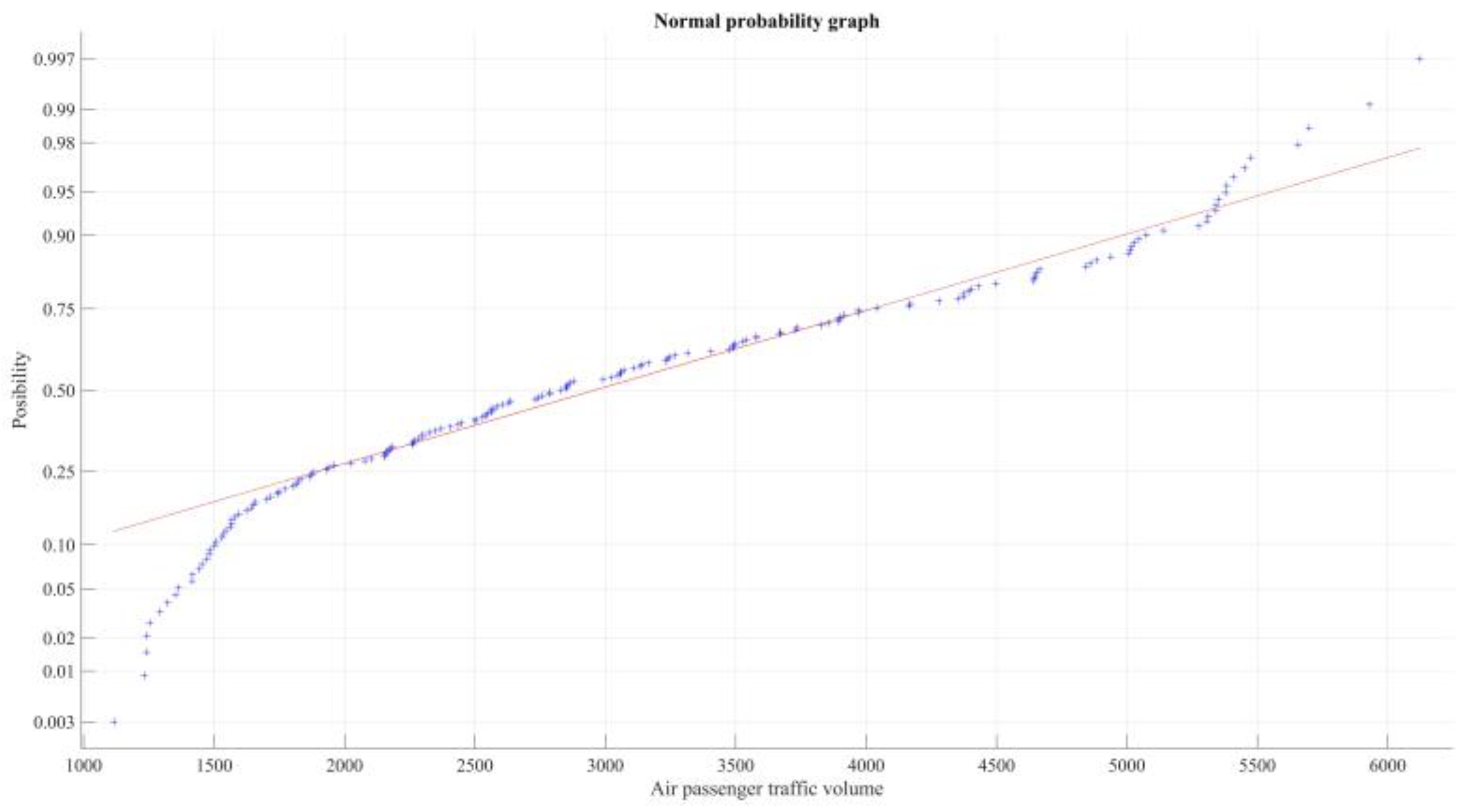
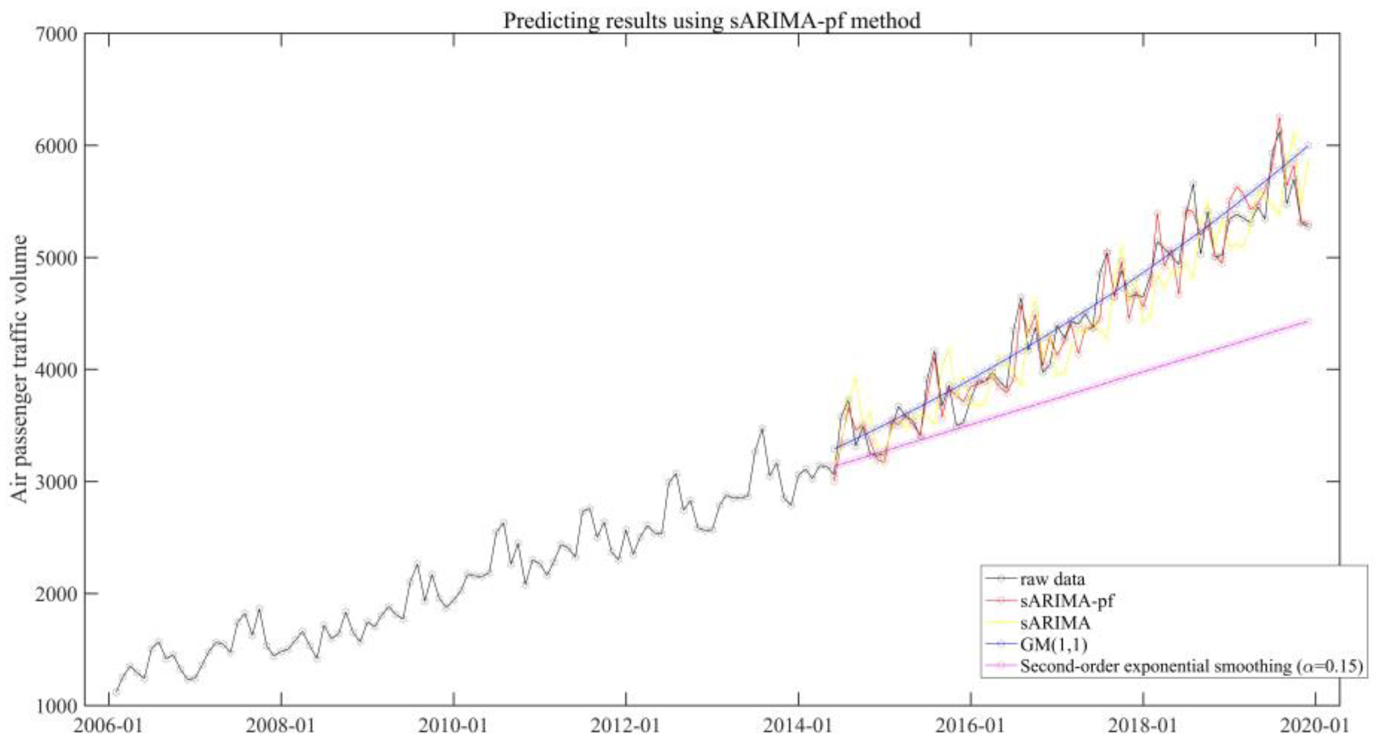
3.2. Case Study of Air Passenger Traffic Volume Prediction

The performance of the proposed sARIMA-pf method was tested using the data from before the outbreak of COVID-19 to obtain a comparable result with the conventional methods. There were 167 data points before the outbreak of COVID-19. The data is from February 2006 to December 2019 and the first step was to build the sARIMA models.

Seasonality can be identified by a visual examination of the data sequence, using the autocorrelation function (ACF) and the partial autocorrelation function (PACF). The result of ACF displays the time lag on the horizontal axis and the vertical axis displays the autocorrelation coefficient.

The result of ACF on the raw data from February 2006 to December 2019 is displayed in Figure 3 and Figure 4, from which it can be seen that ACF of the raw data is not rapid convergence to the threshold value, which means the raw data is not stable and cannot be used to build ARMA model directly. The raw data should be calculated by the differential function.

The differential data is shown in Figure 5. It can be seen that the trend is wiped off and the periodic fluctuation is retained compared with the raw data shown in Figure 1. By conducting the ACF on the differential data, as shown in Figure 6, we can find that the differential data display rapid convergence to the threshold value, which means that the differential data is stable. The largest peak arises where the lag equals 12, which proves the data is seasonal and suitable for modeling by sARIMA. The seasonal period is set as 12.

Practically, the simplest model that adequately represents the problem should be used [25]. This means that the forecasting model should use the least number of parameters to avoid overfitting. The Akaike information criterion (AIC) and Schwarz’s Bayesian information criterion (BIC) were used in this work. AIC and BIC can by calculated by

$$\begin{array}{l}AIC=N\log (\frac{SSE}{N})+2(k+2)\\ BIC=N\log (\frac{SSE}{N})+(k+2)\log (N)\end{array}$$

(19)

where $SSE$ is the sum of squared errors and $k$ is the number of parameters in the model. The results are given in

Table 1. ARIMA models and results.

Model	AIC	BIC	Model	AIC	BIC
ARIMA(1,1,1)	1.9040	1.9131	ARIMA(3,1,1)	1.9052	1.9203
ARIMA(1,1,2)	1.8971	1.9093	ARIMA(3,1,2)	1.9072	1.9254
ARIMA(1,1,3)	1.9058	1.9210	ARIMA(3,1,3)	1.9086	1.9298
ARIMA(1,1,4)	1.9061	1.9243	ARIMA(3,1,4)	1.8900	1.9142
ARIMA(2,1,1)	1.9040	1.9161	ARIMA(4,1,1)	1.9049	1.9232
ARIMA(2,1,2)	1.9048	1.9200	ARIMA(4,1,2)	1.8994	1.9207
ARIMA(2,1,3)	1.8996	1.9178	ARIMA(4,1,3)	1.8964	1.9207
ARIMA(2,1,4)	1.8997	1.9210	ARIMA(4,1,4)	1.8909	1.9183

. Since the minimum value of AIC occurs when the order of AR is 3 and the order of MA is 4, ARIMA(3,1,4) is selected as the model. The distribution of air passenger traffic volume after using the differential method is shown in Figure 7, from which we can find that it satisfies the normal distribution. Then, sARIMA(3,1,4) (1,1,1)₁₂, is set as the model for the proposed framework.

Then, the sARIMA can be used to build the sARIMA-pf model by the steps proposed in Section 2.4. One hundred of the 167 data points (from February to May 2014) were used as the modeling data to build both the sARIMA model and the sARIMA-pf model. To better illustrate the effectiveness of the proposed method, the Grey model GM (1,1) [14] and the second-order exponential smoothing model [4] with a smoothing factor $\alpha =0.15$ were also trained with the same data. The rest of the data were used to test the performance of the models. Both MSE and RMSE were calculated, and the results are given in

Table 2. Errors from the models under the conventional scenario.

Model	MSE	RMSE
GM(1,1)	62,166	249.3309
Second-order exponential smoothing with $\alpha =0.15$	513,140	716.3373
sARIMA	111,850	334.4425
sARIMA-pf	28,759	169.5857

. The proposed sARIMA-pf model displays smaller error than the other models, which means that the proposed sARIMA-pf model performs better than the other models under the conventional scenario, as shown in Figure 8. Compared with the sARIMA model, the sARIMA-pf model promotes the accuracy by 49.29% evaluated using RMSE.

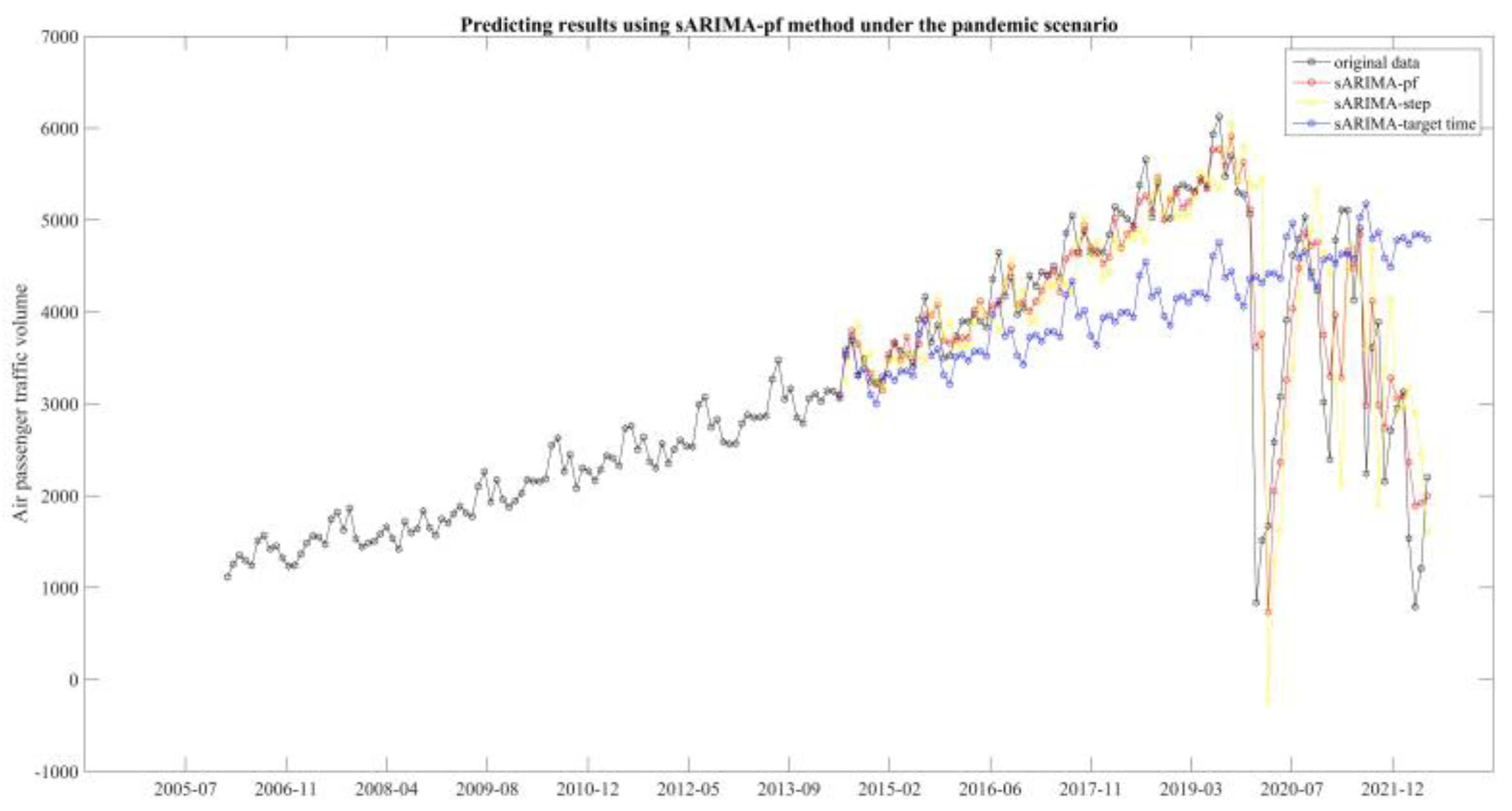
3.3. Case Study of Air Passenger Traffic Volume Prediction under the Pandemic Scenario

This case study shows the performance of the proposed sARIMA-pf model under the influences of COVID-19. As a comparison, the performance of sARIMA was tested first. As shown in Figure 9, 167 of the 197 data points (from February 2006 to December 2019) were used to build the sARIMA model, and the 95% confidence interval was given by the green and red lines. The sARIMA model fails to predict the sharp decrease shown by the yellow line caused by the COVID-19 from January 2020. It is easy to deduce that when the number of the data used to build the model increases, the sARIMA model still cannot work under the scenario without employing external information, which can be regarded as the disadvantage of using the time series to conduct the target-time prediction.

A step-by-step prediction was also conducted, and the result is shown in Figure 10. One hundred of the 197 data points were used to build the initial models. In this part, each newly obtained observation was integrated into the models. For the sARIMA model, each time the model is rebuilt using all the known information at the predicting time point, which is called step-by-step prediction. The step-by-step prediction result of sARIMA model is given by the yellow line shown in Figure 10. The Grey model GM (1,1) and the second-order exponential smoothing model were tested with the same strategy. As a comparison, the result of the target-time prediction using the sARIMA model, the Grey model GM (1,1), and the second-order exponential smoothing model are given by the blue, cyan, and purple lines. Obviously, all the three models failed in conducting the target-time prediction.

The sARIMA-pf model shows great advantages compared with the sARIMA model, the Grey model GM (1,1), and the second-order exponential smoothing model. In Figure 10, the sARIMA-pf model achieves better performance following the data points after the outbreak of COVID-19. To evaluate the performance, MSE and RMSE was calculated and listed in

Table 3. Errors from the models under the pandemic scenario.

Model	MSE	RMSE
GM(1,1)	14,940,000	3865.3
Second-order exponential smoothing with $\alpha =0.15$	11,395,000	3375.6
sARIMA-pf	295,030	543.1681
sARIMA-target time	1,606,400	1267.4
sARIMA-step-by-step	973,740	986.7838

. The result shows that the sARIMA-pf model performs better than the sARIMA model predicted step-by step and far better than the other models. For the certain scenario, sARIMA-pf model promotes the accuracy by 44.96% evaluated using RMSE compared with the sARIMA model.

4. Conclusions

This paper proposed a novel framework to cope with the air-transport demand forecast task considering uncertainties caused by accidental factors. Combined with the particle filter method, an sARIMA model was selected as the basic model of the framework to build a novel sARIMA-pf model. The performance of the proposed method was verified in different air passenger traffic volume prediction scenarios. For the conventional scenario without the influences by the outbreak of COVID-19, the proposed method increased the accuracy by 49.29%, evaluated using RMSE compared with sARIMA model. For the pandemic scenario considering the accidental factors, the proposed method increased the accuracy by 44.96%, evaluated using RMSE compared with the sARIMA model. The proposed method was verified to be effective on multi-scenario prediction.

One of the main contributions of this work is that the applicability of a high-order sARIMA used as the state transition model of the particle filter framework is shown and the effectiveness is proved. For traditional particle filter based predicting frameworks, the state transition models are represented by one-order recursive models, and such types of models cannot be used for the air-transport-demand forecasting considering the seasonal periodicity of the data. The proposed high-order sARIMA method can further be used in other engineering areas, such as the failure prediction of mechanical parts, if the conditions which are required by ARIMA-like models are satisfied.

References

1. Li, X.; de Groot, M.; Bäck, T. Using forecasting to evaluate the impact of COVID-19 on passenger air transport demand. Decis. Sci. 2021, 1–16. [Google Scholar] [CrossRef] [PubMed]
2. Kitsou, S.P.; Koutsoukis, N.S.; Chountalas, P.; Rachaniotis, N.P. International Passenger Traffic at the Hellenic Airports: Impact of the COVID-19 Pandemic and Mid-Term Forecasting. Aerospace 2022, 9, 143. [Google Scholar] [CrossRef]
3. National Academies of Sciences. Engineering, and Medicine. Addressing Uncertainty about Future Airport Activity Levels in Airport Decision Making. 2012. Available online: https://nap.nationalacademies.org/catalog/22704/addressing-uncertainty-about-future-airport-activity-levels-in-airport-decision-making (accessed on 22 March 2022).
4. Spitz, W.; Golaszewski, R. Airport Aviation Activity Forecasting; Transportation Research Board: Washington, DC, USA, 2007. [Google Scholar]
5. Box, G.E.; Jenkins, G.M.; Reinsel, G.C.; Ljung, G.M. Time Series Analysis: Forecasting and Control; John Wiley & Sons: Hoboken, NJ, USA, 2015. [Google Scholar]
6. Williams, B.M.; Durvasula, P.K.; Brown, D.E. Urban freeway traffic flow prediction: Application of seasonal autoregressive integrated moving average and exponential smoothing models. Transp. Res. Rec. 1998, 1644, 132–141. [Google Scholar] [CrossRef]
7. Andreoni, A.; Postorino, M.N. A multivariate ARIMA model to forecast air transport demand. Proc. Assoc. Eur. Transp. Contrib. 2006, 1–14. [Google Scholar]
8. Tsui WH, K.; Balli, H.O.; Gilbey, A.; Gow, H. Forecasting of Hong Kong airport’s passenger throughput. Tour. Manag. 2014, 42, 62–76. [Google Scholar] [CrossRef]
9. Barczak, A.; Dembińska, I.; Rozmus, D.; Szopik-Depczyńska, K. The Impact of COVID-19 Pandemic on Air Transport Passenger Markets-Implications for Selected EU Airports Based on Time Series Models Analysis. Sustainability 2022, 14, 4345. [Google Scholar] [CrossRef]
10. Zhu, X.; Lin, Y.; He, Y.; Tsui, K.-L.; Chan, P.W.; Li, L. Short-Term Nationwide Airport Throughput Prediction With Graph Attention Recurrent Neural Network. Front. Artif. Intell. 2022, 105. [Google Scholar] [CrossRef] [PubMed]
11. Utku, A.; Kaya, S.K. Multi-layer perceptron based transfer passenger flow prediction in Istanbul transportation system. Decis. Mak. Appl. Manag. Eng. 2022, 5, 208–224. [Google Scholar] [CrossRef]
12. Lin, G.; Lin, A.; Gu, D. Using support vector regression and K-nearest neighbors for short-term traffic flow prediction based on maximal information coefficient. Inf. Sci. 2022, 608, 517–531. [Google Scholar] [CrossRef]
13. Jin, F.; Li, Y.; Sun, S.; Li, H. Forecasting air passenger demand with a new hybrid ensemble approach. J. Air Transp. Manag. 2020, 83, 101744. [Google Scholar] [CrossRef]
14. Wong, H.L. Time series forecasting with stochastic Markov models based on fuzzy set and grey theory. In Applied Mechanics and Materials; Trans Tech Publications Ltd.: Wollerau, Switzerland, 2015; pp. 975–978. [Google Scholar]
15. Meng, H.; Geng, M.; Xing, J.; Zio, E. A hybrid method for prognostics of lithium-ion batteries capacity considering regeneration phenomena. Energy 2022, 261, 125278. [Google Scholar] [CrossRef]
16. Song, W.; Wang, Z.; Li, Z.; Han, Q.-L. Particle-Filter-Based State Estimation for Delayed Artificial Neural Networks: When Probabilistic Saturation Constraints Meet Redundant Channels. IEEE Trans. Neural Netw. Learn. Syst. 2022, 1–9. [Google Scholar] [CrossRef] [PubMed]
17. Li, T.; Wang, S.; Zio, E.; Shi, J.; Ma, Z. A numerical approach for predicting the remaining useful life of an aviation hydraulic pump based on monitoring abrasive debris generation. Mech. Syst. Signal Process. 2020, 136, 106519. [Google Scholar] [CrossRef]
18. Tongyang, L.; Shaoping, W.; Jian, S.; Zhonghai, M. An adaptive-order particle filter for remaining useful life prediction of aviation piston pumps. Chin. J. Aeronaut. 2018, 31, 941–948. [Google Scholar]
19. Chen, J.; Ma, C.; Song, D.; Xu, B. Failure prognosis of multiple uncertainty system based on Kalman filter and its application to aircraft fuel system. Adv. Mech. Eng. 2016, 8, 1687814016671445. [Google Scholar] [CrossRef] [Green Version]
20. Zio, E.; Peloni, G. Particle filtering prognostic estimation of the remaining useful life of nonlinear components. Reliab. Eng. Syst. Saf. 2011, 96, 403–409. [Google Scholar] [CrossRef]
21. Hassani, S. Dirac delta function. In Mathematical Methods; Springer: Berlin, Germany, 2009; pp. 139–170. [Google Scholar]
22. Zhang, G.P. Time series forecasting using a hybrid ARIMA and neural network model. Neurocomputing 2003, 50, 159–175. [Google Scholar] [CrossRef]
23. Hyndman, R.J.; Athanasopoulos, G. 8.9 Seasonal ARIMA models. Forecast. Princ. Practice. Otexts. Retrieved 2015, 19. [Google Scholar]
24. Schneider, R.; Chen, X. Predicting Flight Demand under Uncertainty. KSCE J. Civ. Eng. 2020, 24, 635–646. [Google Scholar] [CrossRef]
25. McLeod, A.I. Parsimony, Model Adequacy and Periodic Correlation in Time Series Forecasting; International Statistical Institute: The Hague, The Netherlands, 1993; pp. 387–393. [Google Scholar]
Figure 1. The raw data.
Sustainability 14 16694 g001
Figure 2. The distribution of the growth rate of the air passenger traffic volume.
Sustainability 14 16694 g002
Figure 3. The autocorrelation function result of the raw data.
Sustainability 14 16694 g003
Figure 4. The partial autocorrelation function result of the raw data.
Sustainability 14 16694 g004
Figure 5. The differential data.
Sustainability 14 16694 g005
Figure 6. The autocorrelation function result of the differential data.
Sustainability 14 16694 g006
Figure 7. The distribution air passenger traffic volume using the differential method.
Sustainability 14 16694 g007
Figure 8. The predicting result using sARIMA-pf method.
Sustainability 14 16694 g008
Figure 9. The predicting results using sARIMA under the pandemic scenario.
Sustainability 14 16694 g009
Figure 10. The predicting results using sARIMA-pf method under the pandemic scenario.
Sustainability 14 16694 g010