3.3.1. Determination of Influencing Factors
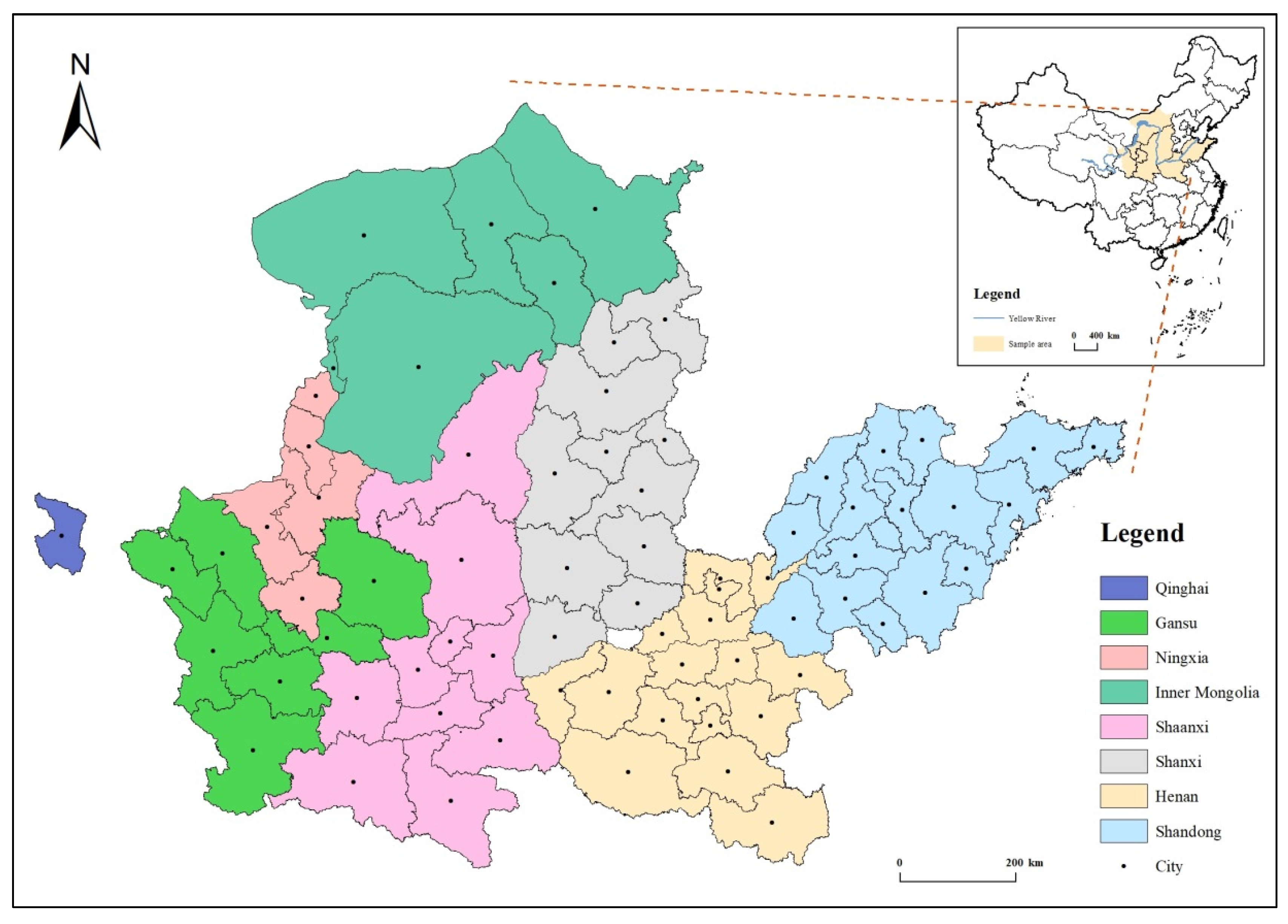
The evolution of PLES is affected by multiple factors. The research area includes 73 cities in eight provinces, each with a different development status. Based on this, the index system of PLES in the YRB was constructed by selecting variables from four dimensions: government governance, social economy, population restriction and industrial structure. Finally, eight variables were selected to explore the driving mechanism of its evolution (see
Table 6).
Financial revenue. Financial revenue is an important indicator to measure the government’s financial resources, a prerequisite and condition for the government to carry out public expenditure, and an important means for the government to carry out macrocontrol. Local general public budget revenue is fiscal revenue mainly from taxation; it is mainly used to ensure and improve people’s wellbeing and promote economic and social development. Local government planning and the use of administrative areas can change the local general public budget revenue to a certain extent [
32]. Local general public budget revenue can reflect the financial revenue of regional governments.
Environmental greening. Environmental greening is an effective means to optimize the ecological environment. Through urban greening, the government can improve the sanitary conditions of the city and effectively improve the living environment of residents. High-quality development requires urban greening and economic development to promote and coordinate development, and environmental greening will improve the ecological environment [
37,
46] and then affect the evolution of PLES. A green area is a variety of green spaces used for gardening and greening, and it can directly reflect the level of urban environmental greening.
Investment intensity. Investment and economic growth are closely related; investment is the fundamental power of economic growth but also the essential precondition of economic growth. In all aspects of investment, governments and enterprises choose the best land as the target based on the principle of economic maximization [
47]. Fixed asset investment is the workload of fixed asset construction and acquisition activities expressed in monetary terms, which can be a good measure of local investment intensity.
Economic development. In the development of the urban economy, land space needs to be developed and utilized [
48]. Urban economic development can provide more funds and more advanced technologies for land use and provide a reliable guarantee for ecological environment protection, but it may also break the evolution direction and speed of the original PLES. Economic density is derived from the ratio of regional GDP to total area for each city, which can be a more objective measure of the level of economic development of each region.
Population size. Humans are closely related to land, and their productive lives depend on land resources. High economic growth and changes in population numbers have led to a gradual increase in productivity levels and an increase in access to land resources for the productive lives of human beings, leading to an increase in human–land conflicts [
49]. The distribution of the PLES in the YRB is different, and ecological and environmental problems are closely related to the population to a certain extent. To explore the impact of population factors on the evolution of the PLES, this paper selects population density to represent population size. Population density is calculated as the ratio of the annual resident population to the total geographical area.
Land use. With the increase in population, people pay increasing attention to land use efficiency, and the reasonable and efficient use of land is of great significance for sustainable development. Land use intensity is the intensity of a unit of land investment, which directly reflects the impact of human activities on natural ecosystems and is calculated according to the literature [
50]. This paper chooses the intensity of land use to measure people’s land use.
Primary industry. Primary industries mainly include agriculture, forestry, animal husbandry, fishing, etc. The primary industries in the YRB are distributed in most areas, and these industries are highly dependent on land. With the upgrading of industries in various regions, the primary industry is squeezed by space, and its changes influence the evolution of PLES [
32]. This paper selects the proportion of primary industry in GDP to measure the development of the primary industry.
Secondary industry. Secondary industries are mainly mining, manufacturing, construction, etc. The construction and development of these industries need to be based on all kinds of land. With the continuous increase in industrialization in the YRB, the demand for land in the secondary industry is also increasing, forcing PS to play a continuous game with LS and ES [
32,
33]. This paper selects the proportion of secondary industry in GDP to measure the development of the secondary industry.
3.3.4. Spatiotemporal Distribution of Estimation Coefficients of Driving Factors
First, the regression coefficients of the influencing factors of the GTWR model were statistically analyzed, and the table of quartiles and averages was drawn (see
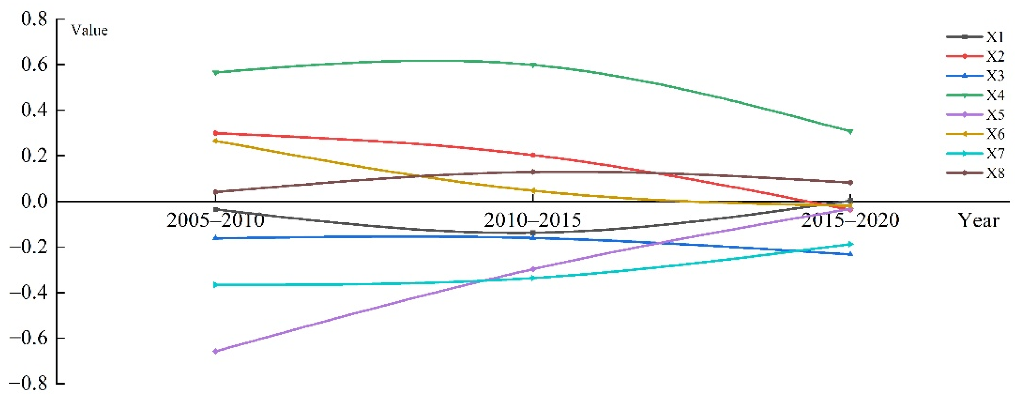
Table 9). The regression coefficients of each influencing factor vary in magnitude, positive and negative, which indicates that the influencing factors have significant nonstationarity on the evolution of the PLES in the YRB in both time and space. Second, the regression coefficients of the impact factors of the GTWR model for 2005–2010, 2010–2015, and 2015–2020 were visualized, and their averages were plotted on a line graph (see
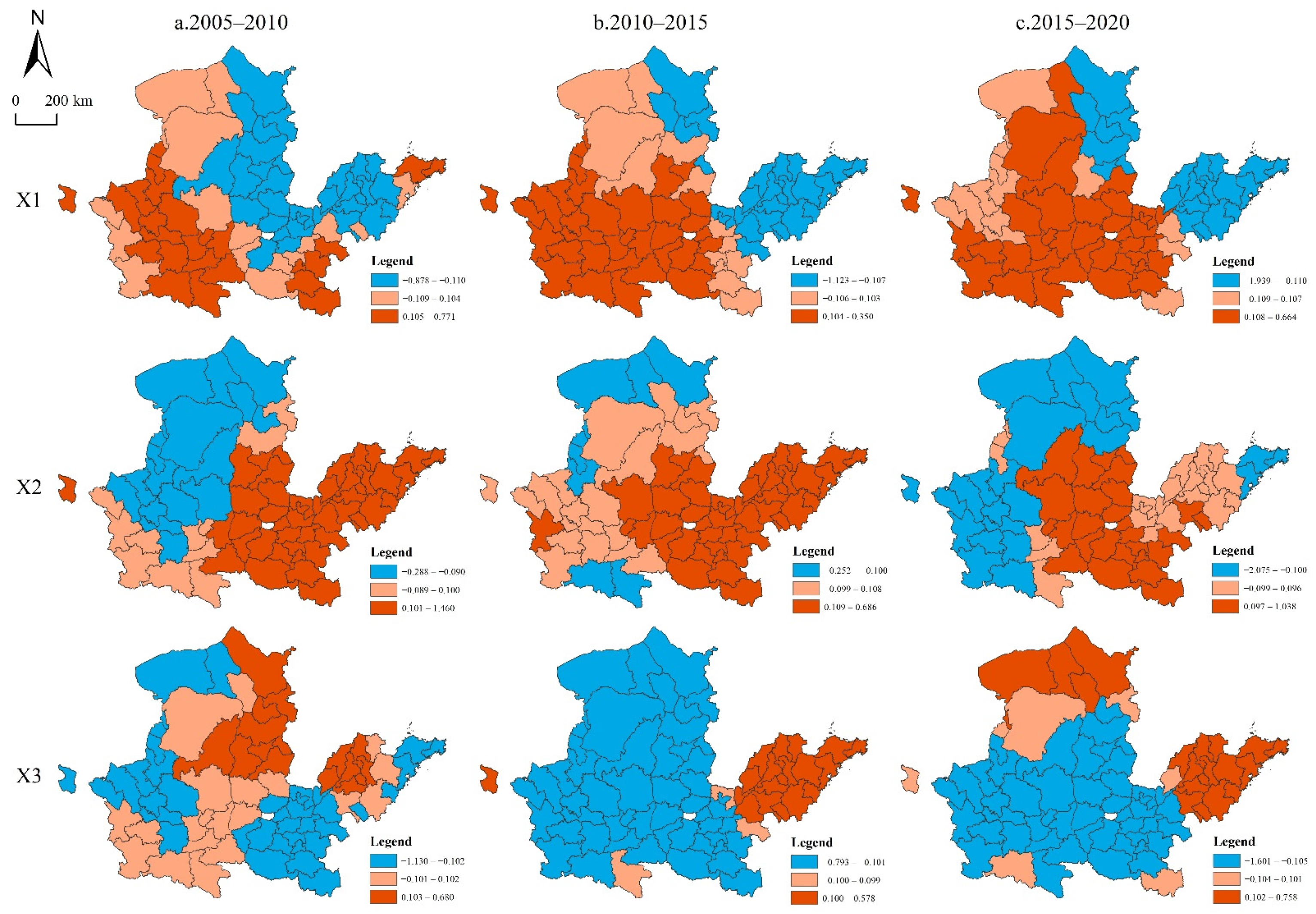
Figure 5) to observe the time change trend. Finally, the regression coefficients of the influencing factors were visualized by ArcGIS 10.2 software, so as to analyze their changing trend in the spatial and temporal dimensions (see
Figure 6).
According to
Table 9, the average regression coefficient of local general public budget revenue is −0.056, with a median of 0.043, indicating that local general public budget revenue has a small negative impact on the evolution of the PLES, and the overall left-biased trend of the coefficients reflects that the index has a positive influence on the spatial evolution of the PLES in most cities. The upper and lower quartiles range from −0.291 to 0.253, indicating that the positive and negative effects of local general public budget revenues are relatively evenly distributed among cities in each year.
In terms of time trends (see
Figure 5), the mean value of the local general public budget revenue regression coefficient is −0.035, −0.137, and 0.004 in 2005–2010, 2010–2015, and 2015–2020, respectively, exhibiting a trend of declining and then increasing. This is because the PLES comprehensive dynamic degree as a whole is first a weakening and then an increasing trend, and as the economic development of each region’s local general public budget revenue grows year by year, the negative effect appears to weaken.
In terms of spatial distribution characteristics (see
Figure 6), the regional distribution of the positive and negative regression coefficients of local general public budget revenue is more fragmented from 2005 to 2020, with the positive regions gradually expanding from west to east and the negative regions gradually shrinking from west to east. The characteristics of the spatial influence of local general public budget revenue on the dynamic degree of the PLES are mainly related to the distribution of the PS. Shandong relies on the geographical advantage of being located near the sea for rapid development. Its PS and LS have been expanding, but its early economic development model was relatively crude, resulting in the continuous reduction of ecological space, and its long-term overall dynamic degree is large, resulting in the local general public budget revenue not being proportional to the development and utilization of land and in a negative area. Ningxia was in a positive region from 2005–2015 and then shifted to an insignificant region. The reason is that local governments compete to attract investment by providing land at low prices to promote economic development, and the land supply strategy tends to help those land supply areas that can quickly and effectively increase the economy [
51]. The gradual expansion of PS promotes the local general public budget revenue, but the shrinkage of ES makes local governments raise their awareness of ES.
- 2.
Environmental greening
According to
Table 9, the average regression coefficient of green area is 0.156, and the median is 0.125, which indicates that green area has a positive influence on the evolution of the PLES, and the coefficient generally has a right-skewed distribution, showing that the positive impact of this index on the evolution of the PLES is small in a few cities. The upper and lower quartiles range from −0.072 to 0.353, which indicates a stronger positive effect of green area in the city in all years.
Regarding the trend of time change (see
Figure 5), from 2005 to 2020, the average of the regression coefficient of green space area was 0.300, 0.203, and −0.037, respectively. The value gradually decreased, indicating that the positive influence of green area on the evolution of the PLES gradually decreased and showed a negative influence in 2015–2020.
In terms of spatial distribution characteristics (see
Figure 6), from 2005 to 2020, the positive and negative regression coefficients of green area are interspersed and change significantly, and its spatial impact distribution characteristics on the dynamic degree of the PLES are mostly connected with the distribution of ES. The positive region is decreasing and shifting from downstream to midstream, with the most obvious change in Shaanxi. Due to the gradual protection of ES [
6], LS is more focused on greening and environmental protection, and long-term soil erosion in the midstream is gradually being managed, with an increasing green area. The negative area tends to decrease first and then increase and is concentrated upstream of the YRB. This is because the upper reaches are mainly ES, the weak awareness of greening construction leads to the trend of shrinking ES, and the LS expands while ignoring the construction of greening.
- 3.
Investment intensity
According to
Table 9, the average regression coefficient of fixed asset investment is −0.185, and the median is −0.193, which indicates that fixed asset investment has a negative influence on the evolution of the PLES. The coefficients generally have a right-skewed distribution, indicating that the index has a strong negative influence on the evolution of the PLES in most cities. The upper and lower quartiles range from −0.423 to 0.086, indicating a stronger negative impact of fixed asset investment in cities in all years.
In terms of time trends (see
Figure 5), the mean value of the regression coefficient of fixed asset investment decreases from −0.162 to −0.233 from 2005 to 2020, which indicates that the negative influence gradually increases because some cities in the YRB with a lower dynamic degree of PLES are investing more.
In terms of spatial distribution characteristics (see
Figure 6), from 2005 to 2020, fixed asset investment is mainly negative, and its spatial impact on the dynamic degree of the PLES is mainly related to the geographical location. Shandong has long been in a positive region because it relies on its unique geographic location, which has developed faster compared to other provinces in the YRB, and because it has a larger share of investment in land. Most of Shanxi was in the positive zone from 2005–2010 because the local government started to strictly regulate enterprises with serious environmental pollution, such as coal mining, banned the unqualified ones, and gradually invested in new industries. Inner Mongolia’s PLES dynamic degree remains relatively stable but in 2015–2020 in a positive region because the local government has increased investment in green energy with the advantage of local resources. Other provinces are basically in the negative region or inconspicuous region because these provinces do not have unique natural resources, resulting in a relatively small land dynamic attitude and mainly traditional industries resulting in a relatively underdeveloped economy. The local government has increased investment in various industries to achieve common prosperity.
- 4.
Economic development
According to
Table 9, the average regression coefficient of economic density is 0.491, and the median is 0.353, which indicates that it has a great positive influence on the evolution of the PLES in general. The coefficient has a right-skewed distribution in general, indicating that the positive influence of this index on the evolution of the PLES in a few cities is small. The upper and lower quartiles range from 0.036 to 0.876, indicating that the economic density of cities has a predominantly positive influence in each year. The regression coefficients of Shuozhou city, Ulanqab city and Datong city in 2015–2020 are greater than 3. The reason is that in recent years, Shuozhou city and Datong city have relied on their traditional resource advantages to accelerate the construction of a green and diversified energy supply system and have gradually realized the new type of coal resource development, while Ulanqab city has relied on its resource endowment to vigorously develop clean energy, and this reform has greatly driven economic development.
In terms of time trends (see
Figure 5), the mean value of the regression coefficient of economic density decreases from 0.566 to 0.307 from 2005 to 2020, indicating that the positive effect gradually diminishes. The possible reason is that the dependence of economic growth on land gradually decreases.
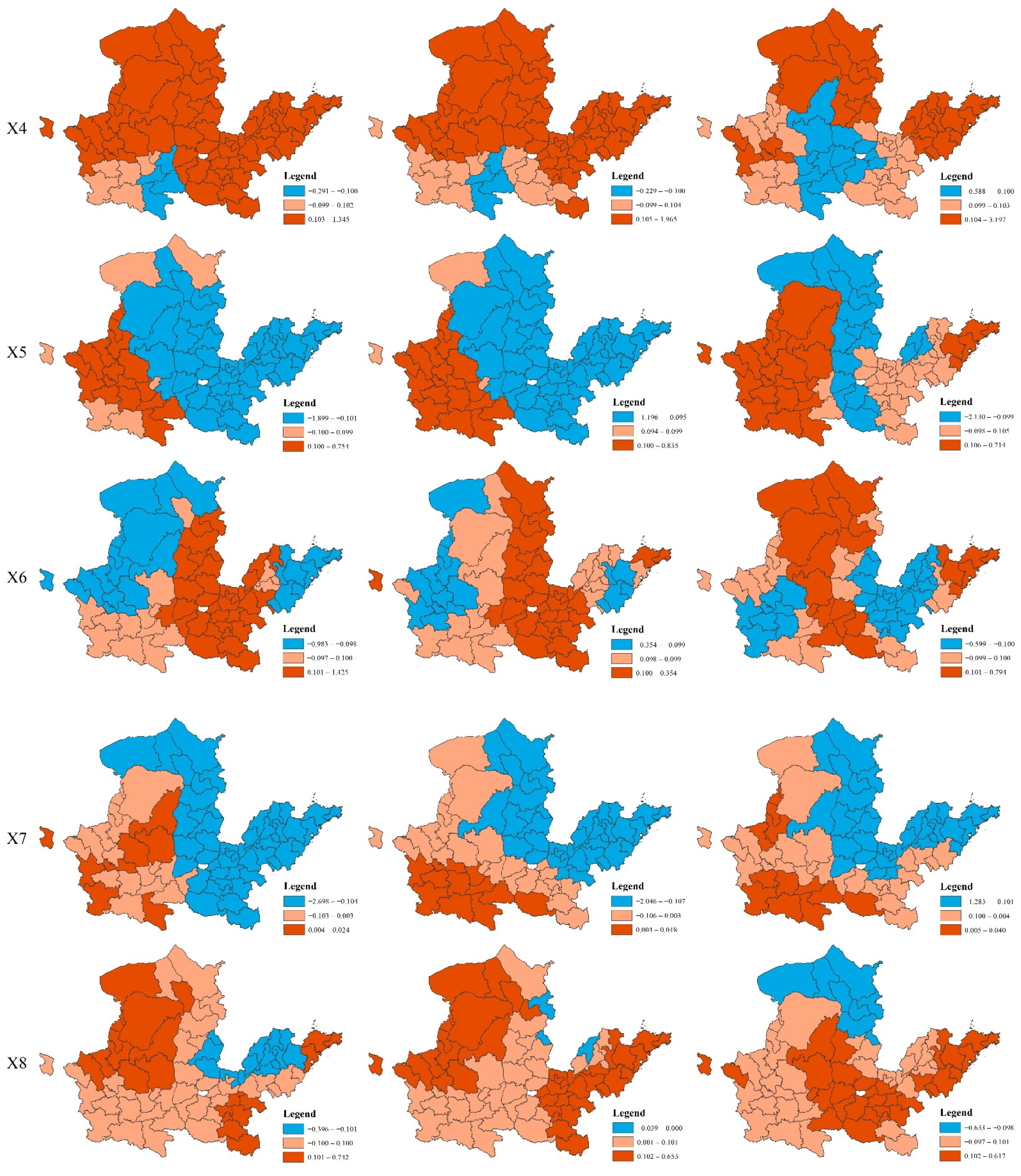
In terms of spatial distribution characteristics (see
Figure 6), economic density is dominated by positive effects from 2005 to 2020, with positive regions decreasing and negative regions increasing with the evolution of time. The spatial influence of economic density on the dynamic degree of the PLES is mostly connected with the economic development pattern. The reason for the gradual expansion of negative areas in Shaanxi is that these areas have long been in ecologically fragile zones. In response to the strategy of “ecological protection and high-quality development of the Yellow River Basin”, local governments have increased the improvement of the ecological environment, which, however, has affected the local economic development. Inner Mongolia, Shandong, and Shanxi have been in positive regions for ages, indicating that the economic development of these regions is coordinated with the PLES dynamic degree [
52]. However, the ES in most areas of the YRB is in a state of shrinkage due to the excessive pursuit of economic effects at the expense of environmental protection.
- 5.
Population size
According to
Table 9, the mean regression coefficient of population density is −0.329, and the median is −0.200, indicating that population density has a large negative influence on the evolution of the PLES. The coefficient generally has a left-skewed distribution, indicating that this index has a large negative influence on the evolution of the PLES in most cities. The upper and lower quartiles range from −0.728 to 0.147, indicating that the negative effect of population density is more significant in each year.
In terms of time trends (see
Figure 5), the mean value of the population density regression coefficient decreases from −0.658 to −0.032 from 2005 to 2020, indicating that the negative effect is weakening. As the population increases, LS needs to expand, and PS needs to deliver more resources and services to people, which also puts great pressure on ES [
53]. However, with the gradual slowdown of the population growth rate and the continuous improvement of population quality, the influence of population density on the evolution of the PLES gradually decreases.
In terms of spatial distribution characteristics (see
Figure 6), from 2005 to 2020, population density is dominated by negative effects, the positive area is mainly concentrated in the upstream and expanding to the midstream, and negative areas gradually are decreasing and shifting from the lower to the middle reaches. The spatial influence of population density on the dynamic degree of the PLES is mainly related to the distribution of LS. Population growth in the upper reaches poses a challenge to the LS, which has to be expanded. The downstream LS is more adequate to meet the growth of population density, and the dynamic degree of the PLES is mainly focused on the PS.
- 6.
Land use
According to
Table 9, the average regression coefficient of land use intensity is 0.099, and the median is 0.004, which indicates that it has a small positive impact on the evolution of the PLES in general. The coefficient generally has a right-skewed distribution, indicating that this index has a small positive impact on the evolution of the PLES in most cities. The upper and lower quartiles range from −0.152 to 0.243, indicating that the positive and negative impacts of land use intensity are more balanced among cities in each year.
In terms of time trends (see
Figure 5), the average of the regression coefficient of land use intensity decreases from 0.266 to −0.019 from 2005 to 2020, indicating that the positive effect gradually decreases. The greater the human development and investment in land are, the greater the land use intensity. With the progress of land development technology and the awareness of high-quality development, land use efficiency gradually increases.
In terms of spatial distribution characteristics (see
Figure 6), the regional distribution of the positive and negative regression coefficients of land use intensity in 2005–2020 is relatively dispersed, and its spatial influence on the dynamic degree of the PLES is mainly related to resource endowment. Shanxi in 2005–2015 was a positive region because Shanxi is a large province of coal resources, and land use intensity also caused damage to the ecological environment. In 2015–2020, the positive region significantly decreased because the implementation of ecological and environmental protection continued to eliminate some of the unqualified enterprises, and PS also appeared to shrink. Most of the upper YRB was in the negative region from 2005–2015 because the economic development of the upper reaches depended on the many natural resources given by the ecological environment and people had been using the land with low intensity for a long time. The negative area decreased from 2015 to 2020 because, with the implementation of the “development of the western region in China” policy, the layout of the PLES in the upper reaches of the YRB has changed.
- 7.
Primary industry
According to
Table 9, the average regression coefficient of the proportion of primary industry in GDP is −0.297, and the median is −0.140, which indicates that it has a negative impact on the evolution of the PLES in general. The coefficient has a left-skewed distribution in general, indicating that the negative impact of this index on the evolution of the PLES in a few cities is small. The upper and lower quartiles range from −0.383 to −0.013, indicating that the influence of the proportion of primary industry in GDP is mainly negative in each year. The regression coefficients of Weihai city and Yantai city were in the range of −2.698 to −1.934 from 2005 to 2015 because Weihai city and Yantai city relied on the advantages of the seafront to develop port shipping vigorously, and even reclamation of land occurred during this period [
54]. With the implementation of the coastal protection law, however, this behaviour was resisted.
In terms of time trends (see
Figure 5), the average of the regression coefficient of the proportion of primary industry in GDP decreases from −0.366 to −0.188 from 2005 to 2020, indicating that the negative influence gradually decreases. The primary industry is the basis of people’s lives and the national economy; therefore, the overall layout of the primary industry does not change significantly, but its proportion of GDP gradually decreases.
In terms of spatial distribution characteristics (see
Figure 6), from 2005 to 2020, the positive impact of the proportion of primary industry in GDP decreases along a south-to-north gradient, and the negative impact increases along a south-to-north gradient. Over time, the positive impact area increases, and the negative impact area decreases. The distribution characteristics of the spatial influence of the proportion of primary industry in GDP on the dynamic degree of the PLES are mainly related to the distribution of the primary industry. Positive regions are scattered in Gansu and Shaanxi because these regions have a wide distribution of primary industries but generate limited GDP and are in a lower position within the YRB; with the changing spatial pattern of LS, PS and ES and the increase in GDP creation in the primary sector, the upstream is shifting to the region continuously. Shanxi has been in a negative region for a long time because it is dominated by the mining industry [
55], the primary industry is less distributed, and the exploitation of land by the mining industry has a continuous impact on the PLES.
- 8.
Secondary industry
According to
Table 9, the average regression coefficient of the proportion of secondary industry in GDP is 0.085, with a median of 0.084, showing that it has a positive effect on the evolution of the PLES, without a significantly skewed distribution. The minimum value is −0.633, and the maximum value is 0.742, with a small difference in the extreme values. The upper and lower quartiles range from 0.027 to 0.162, indicating that the influence of the proportion of secondary industry in GDP on the evolution of the PLES is mainly positive.
Regarding the trend of time change (see
Figure 5), the average regression coefficient of the proportion of secondary industry in GDP from 2005 to 2020 is 0.041, 0.130 and 0.084, respectively, which increased first and then decreased because, in recent years, the proportion of tertiary industry in GDP has increased due to the green and efficient development and structural upgrading of the secondary industry.
In terms of spatial distribution characteristics (see
Figure 6), from 2005 to 2020, the proportion of secondary industry in GDP has mainly positive effects, and its spatial impact on the dynamic degree of PLES is mainly related to the distribution of secondary industry. Positive regional contraction from the edge to the centre is because most of the YRB relies on cheap human resources and land, making for the gradual expansion of the secondary industry, which gradually increases in the central region along with the implementation of “The Rise of Central China” policy. Inner Mongolia is the most obvious negative region in 2015–2020 because Inner Mongolia relies on the vast land and other advantages to attract a large number of investors and vigorously develop its secondary industry.


