Article

Characteristics and Hazards Analysis of Vortex Shedding at the Inverted Siphon Outlet

1
School of Water Conservancy, North China University of Water Resources and Electric Power, Zhengzhou 450045, China
2
Collaborative Innovation Center of Water Resources Efficient Utilization and Protection Engineering, Zhengzhou 450045, China
3
Henan Hydraulic Structure Safety Engineering Technology Research Center, Zhengzhou 450045, China
4
POWERCHINA Northwest Engineering Corporation Limited, Xi’an 710065, China
*
Author to whom correspondence should be addressed.
Sustainability 2022, 14(22), 14744; https://doi.org/10.3390/su142214744
Submission received: 10 October 2022 / Revised: 31 October 2022 / Accepted: 3 November 2022 / Published: 9 November 2022

Abstract

:
This paper studies Karman vortex shedding and water-level fluctuation in the inverted siphon structure of the Middle Route of the South-to-North Water Diversion Project (MR-SNWDP) in China. Field investigations and numerical simulations for the inverted siphon outlet were performed to explore the characteristics and hazards of the vortex. Numerical results were compared with measured data to verify the effectiveness and reliability of the model. Based on the model, it is found that the periodic water-level fluctuations caused by the Karman vortex street will not only excite surges to beat the gate but will also induce periodical force on the gate pier. Those will damage the building structure and affect the delivery capacity in the long-term operation. Based on this, countermeasures of altering different pier tail shapes are proposed to control vortex shedding, and the effect is noticeable. The study presents a hydraulic process for the inverted siphon outlet and provides a theoretical reference for water delivery safety of inverted siphons and similar structures in MR-SNWDP.

1. Introduction

The Middle Route of the South-to-North Water Diversion Project (MR-SNWDP) aims to optimize the spatial allocation of water resources in North China. It not only guarantees living water for the residents of the northern cities, but also improves the ecological environment of the rivers along the project line through ecological water replenishment [1,2]. With the increasing demand for water resources in North China, the water flow delivery rate through the MR-SNWDP has increased since April 2020. However, a large flow rate results in the water level fluctuating violently at the inverted siphon outlet and the vortex constantly shedding behind the gate pier. When the gate was fully opened, waves continuously beat the gates and the bottom of the lock chamber with a regular “poof” sound, which may cause structure vibration and reduce its safe service life. Moreover, the vortices at the outlet further deteriorate the flow state in the inverted siphon and lessen the water delivery efficiency.
Vortex shedding is a significant phenomenon in various engineering disciplines and is commonly found in bluff-body structures such as marine risers, bridge piers, and subsea pipelines [3,4]. When a bluff body is placed in the flow field, the fluid separates at the end of the bluff body to form a shear layer. When the Reynolds numbers of the flow exceed a specific value, the shear layer further detaches periodically from the surface in the form of vortices and flows downstream along the main flow. Separated by the bluff body, the flow forms periodic vortices in the flow field called the Karman vortex street [5]. Since the discovery of the Karman vortex street, the mechanism of vortex shedding and wake characteristics have been extensively studied [6,7,8], including the distribution of flow velocity and pressure around the cylinder [9,10] and in the wake flow [11,12,13]. The periodic Karman vortex streets also lead to vibrations in structures and objects. Hence, many methods have been tried to control and suppress vortex shedding. Gerrard [14] studied the shedding vortex behind piers with different cross-sectional shapes and found that the vortex shedding was affected by the shape of the pier ends. Wang et al. [15] found that the streamlined blunt body structure can significantly reduce lift and drag and change the frequency of vortex shedding, and thus used a water-drop-shaped fairing to control the wake behind the cylinder. The above research played a marked role in disclosing the vortex shedding mechanism and wake characteristics. So far, vortex behavior in the inverted siphon has not been investigated.
Vortex shedding has been widely investigated by different methods in the past. Wang et al. [16] experimentally investigated the effect of vortex shedding on an aqueduct structure. Apart from the experiments, there have been an increasing number of studies on vortex shedding based on CFD tools. The CFD method has the advantages of lower costs and higher efficiency than the experimental method. Aghaee et al. [17] successfully simulated the flow around a semi-conical pier in the channel bed by a numerical method. Park et al. [18] simulated the wake behind the square column with the standard k ε and RNG k ε turbulence models, and the comparisons of simulation and theory showed that the errors of maximum velocity difference and the drag coefficient ratio were less than 4% when using the RNG k ε model. Most available numerical simulations of flow behavior around piers are performed using the Reynolds-averaged Navier–Stokes equation (RANS) models [19,20,21]. However, compared with other turbulent closure models, i.e., standard k ε , RNG k ε , and realizable k ε , the RNG model can better characterize the unstable coherent turbulence at a high Reynolds number [22,23]. Thus, it is a reliable and efficient method to investigate a turbulent flow.
Overall, Karman vortex shedding has been widely studied before. There have been several studies on wake structures and vortex-induced vibrations. Existing experimental and numerical investigations of vortex shedding were devoted to the response of the pier and flow behavior. However, most of these focused predominantly on the case in an open space, with less attention paid to the more practical case in the limited space. Research on the flow characteristics and hazards of vortex shedding in the inverted siphon is still quite limited.
In this paper, we took a typical inverted siphon of the MR-SNWDP as the research object. The analysis aimed at investigating the occurrence of vortex shedding at the inverted siphon outlet and revealing the mechanism of fluctuations and abnormal sounds. This paper is organized as follows: Firstly, a numerical model for the inverted siphon outlet with the RNG k ε turbulence model is built and validated. After that, the vortex’s flow characteristics and corresponding hazards are analyzed using the numerical model. Finally, we propose countermeasures to effectively control the vortex shedding and reveal the relationship between the fluctuation amplitude and the tail length of the gate pier.

2. Numerical Method

2.1. Mathematical Model

The flow system consists of water and air, and both can be regarded as incompressible flows. The general governing equation for an incompressible fluid is the Reynolds-Averaged Navier–Stokes (RANS) equation, which includes the continuity equation and the momentum conservation equation, which are respectively expressed as follows:
u i x i = 0
ρ u i t + ρ u i u j x j = P x i + μ x j u i x j + x j ρ u i u j ¯ + F i
where u i is the average component of the velocity in the x i direction, i , j = 1 , 2 , 3 , t is the time, ρ is the fluid density, P is the pressure, F i is the volume force acting on fluid elements, μ is the fluid kinematic viscosity, and ρ u i u j ¯ is the general term of kinetic energy caused by turbulence, namely, Reynolds stress.
Due to the introduction of Reynolds stress, the two governing (Equations (1) and (2)) are no longer closed. A common way to model the Reynolds stress is to use the Boussinesq eddy viscosity assumption [24]. The Boussinesq assumption is shown below:
ρ u i u j ¯ = μ t u i x j + u j x i 2 3 ρ k + μ t u i x i δ i j
where k is the turbulent kinetic energy, δ i j is the Kronecker delta, and μ t is the eddy viscosity.
A turbulence model needs to be introduced to determine the eddy viscosity. This study adopts the RNG k ε turbulence model, which is better for fluid separation and vortex simulation [25,26,27]. The RNG k ε model is a modified model based on the k ε model. By modifying the viscosity coefficient of turbulent kinetics, vortices and flows with high strain rates and more curved streamlines can be better simulated [28,29].
In the RNG k ε model, μ t is expressed as a function of the turbulent kinetic energy k and the turbulent dissipation rate ε , as seen in the equation below:
μ t = C μ ρ k 2 ε
where k and ε are solved with their transport equations, respectively. The transport equations are as follows:
t ρ k + x i ρ k u i = x j σ k μ e f f k x j + P k ρ ε
t ρ ε + x i ρ ε u i = x j σ ε μ e f f ε x j + C ε 1 ε k P k C ε 2 ρ ε 2 k R ε
where σ k and σ ε are the inverse effective Prandtl numbers corresponding to k and ε , respectively, and both take a value of 1.39. C ε 1 and C ε 2 are respectively 1.42 and 1.68, and μ e f f is the equivalent viscosity coefficient, which is the sum of the molecular viscosity coefficient μ and the fluid eddy viscosity coefficient μ t .
μ e f f = μ + μ t
In Equation (6), P k is expressed as
P k = μ t u i x j u i x j + u j x i
The RNG k ε model has a similar form to the standard k ε model, but the ε equation in the RNG model has an additional term R ε . It represents the effect of the mean strain rate on the turbulent dissipation rate ε . It can significantly improve the simulation accuracy of flow separation and the vortex [30]. R ε is expressed as
R ε = C μ ρ η 3 1 η / η 0 1 + β η 3 ε 2 k
In the above equation, C μ is constant in the high-Reynolds-number flow region and takes the value of 0.0845. The values of β and η 0 are 0.012 and 4.38, respectively. Here, η is the ratio of the turbulent time scale k / ε to the average strain time S, namely:
η = S k ε
where S = 2 S i j S i j , is the modulus of the mean strain rate tensor, and S i j = 1 2 u i x j + u j x i .
To reveal the phenomenon of water fluctuation at the inverted siphon outlet, the volume of fluid (VOF) technique was employed to simulate and calculate [31]. The VOF method is an effective method proposed by Hirt and Nichols [32]. It is a widely used numerical calculation method for tracking the complex air–water interface, which tracks the fluid change in each cell by constructing the function of the fluid volume in the grid cells and the mesh volume. It determines the free surface at the same time. Water, gas, and a mixture of both within the same cell have the same velocity. In each unit, the sum of the volume fraction of water α w and the volume fraction of gas α a is 1, namely:
α w + α a = 1
In a given unit, α w = 1 means that the unit is completely filled with fluid, α w = 0 means that the unit is completely filled with gas, and if 0 < α w < 1 , it means that there is a free liquid surface in the calculation unit [33]. The volume fraction of water α w is determined by the following formula:
α w t + u i α w x i = 0
The water–air interface is traced by solving the continuity Equation (12).

2.2. Model Setup

According to the site investigation, the water surface at the inverted siphon inlet was smooth. There was no local vortex or backflow on the inlet surface. Moreover, the size of the inverted siphon body was uniform. The flow in the inverted siphon is constant under normal operating conditions, and the flow characteristics are the same in all sections. Based on the above factors, only the outlet section, including the lock chamber, the transition section, and a part of the canals, was selected to model and analyze the hydraulic characteristics. The calculation model is shown in Figure 1.
The size of the computational domain is 13.80 m × 5.93 m × 2.94 m (length × width × height), and the computational domain is divided into structural grids. About 930,000 grids with a 0.2 m grid size are present, including 670,000 fluid grids. In Figure 2a, the computational domain is depicted.
To represent the flow conditions, it should carefully define the boundary conditions. As shown in Figure 2b,c, measured flow rates for each case were specified as the upstream boundary condition. The downstream boundary condition adopted a specified velocity. The bottom and sidewalls adopted no-slip wall boundaries, where tangential and normal velocities were zero. The top boundary was normally set to symmetry. The water flow viscosity coefficient was set to 0.001 N·s/m2. The canal roughness was set to 0.014. The total calculation time was set to 1800 s.
After the operation of the MR-SNWDP, the flow rate of the inverted siphon was between 80–100 m3/s most of the time. Under this condition, the buildings in this section operated normally, and there was no abnormal flow state. However, when the water delivery flow rate was 240–270 m3/s, exceeding the design flow of 250 m3/s, water fluctuated at the inverted siphons outlet with regular abnormal noise. In this study, the measured flow rate of 263 m3/s and the measured downstream flow velocity of 1.031 m/s were taken as the upstream and downstream boundary conditions, respectively.

2.3. Model Validation

To verify the accuracy of the numerical model, the hydraulic experimental results, including water depth and flow rate at the inverted siphon outlet, were measured on-site. The instantaneous flow rate of the inverted siphon was 234 m3/s in the field. Measured points were arranged along the left bank at 18.25 m away from the lock chamber section Three measured points were arranged in each lock chamber, including 2 points at 0.5 m from two sidewalls and a mid-point. A total of 9 data points were measured, as shown in Figure 3. Because the water level at the inverted siphon outlet fluctuated violently, each point was measured twice: the highest and lowest water depth, respectively. The specific measured water depth data are shown in Table 1.
The measured example was simulated using the model mentioned above, with an inlet flow rate of 234 m3/s and a downstream velocity of 1.009 m/s. The simulated flow state at the outlet was similar to that recorded on-site, as shown in Figure 4. Figure 5 shows the comparison of water depth between measurement and simulation. The numerical water depths agreed with the measured values, and the errors were less than 4.38%, which is within reasonable limits. As a result, the numerical model may produce accurate results for the water level and the hydrodynamic characteristics.

3. Results and Discussion

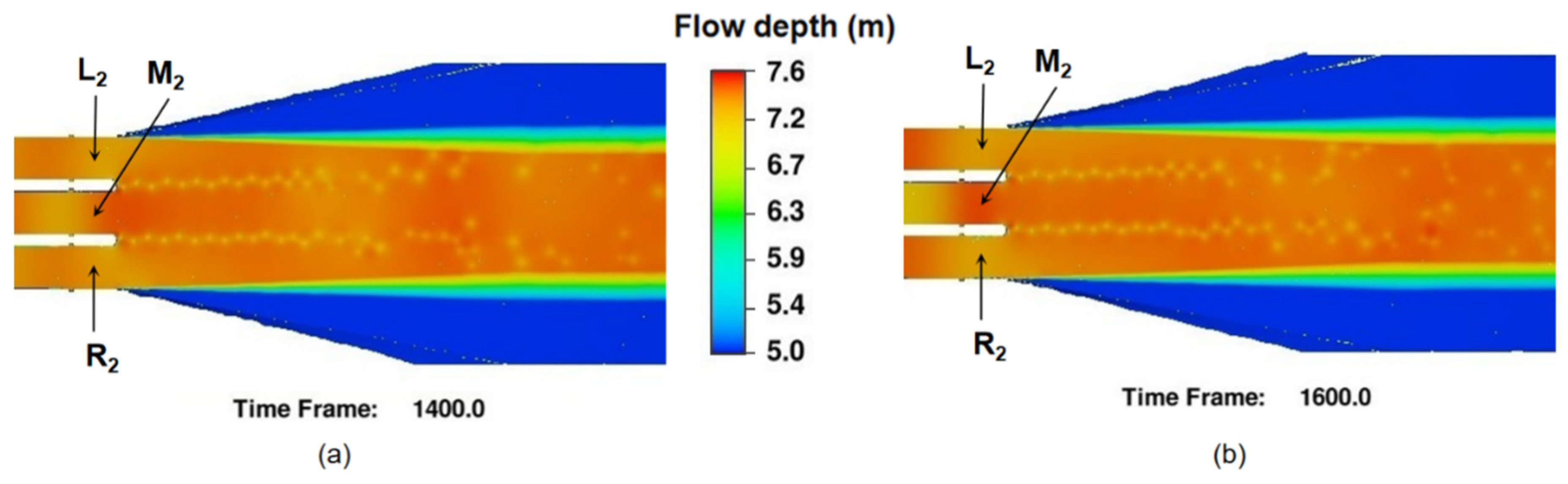
3.1. The Karman Vortex Street at the Outlet

Under fully operating conditions with three opening gates, the flow rate of water delivery reached 263 m3/s. We observed that the water level fluctuated violently and alternately in the three lock chambers. The maximum fluctuation amplitude reached 0.6 m. Moreover, the water flow behind the gate pier periodically oscillated. The vortices shed alternately on the left and right surfaces of the gate piers, and a symmetrical array of the vortex formed in the wake.
Figure 6 reflects a typical process of generation, development, diffusion, and shedding behind two piers. A vortex will first generate on one side and gradually grow larger after the old vortex sheds from the other side of the gate pier (Figure 6a,b). The vortex in the left column rotates clockwise, while in the right column it rotates counterclockwise (Figure 6c). A vortex array with opposite rotation directions and regular arrangement that forms behind a gate pier is known as a “Karman vortex street” [34]. The Karman vortex generates a lateral force on the surrounding water. It obstructs the mainstream and raises the local water level. A wave peak was formed and transmitted upstream (Figure 6d). The Karman vortex street that periodically sheds behind the gate pier is the primary reason for the water-level fluctuation. As the vortex alternately sheds, the water surface will alternately lift and lower.
Figure 7 shows the flow velocity distribution at the inverted siphon outlet at two moments. This region’s maximum flow velocity is close to 2.5 m/s. The large flow velocity is distributed at the gate pier end. Additionally, two rows of vortices behind the two gate piers are distributed symmetrically. The vortex passed downstream with the flow while diffusing around. The strength of the detaching vortex decreased as the vortex moved downstream. Due to the continuous, viscous loss of vortex energy, the vortex decomposed into a random turbulent flow when it moved to the transition section end.
The flow section dramatically increases when fluid passes through the semicircular pier, while the velocity of the boundary layer drops. The boundary layer along the wall transforms into the shear layer, then separates at the end of the pier due to an adverse pressure gradient. A vortex is created when a significant volume of fluid is drawn into the separation zone, and the Karman vortex street is produced. The regime of the Karman vortex street is related to the incoming velocity, fluid viscosity, and structure size (such as diameter), which can be characterized by the Reynolds number R e [35]. When 3 × 10 2 < R e < 3 × 10 5 , the vortex street is fully turbulent in the flow field; when 3 × 10 5 < R e < 3 × 10 6 , the wake is narrower and disorganized; and when R e > 3 × 10 6 , the turbulent vortex street re-establishes. Under the fully operating condition, the Reynolds number R e at the inverted siphon outlet is larger than 6 × 10 6 . Thus, a turbulent vortex street forms behind the gate pier.

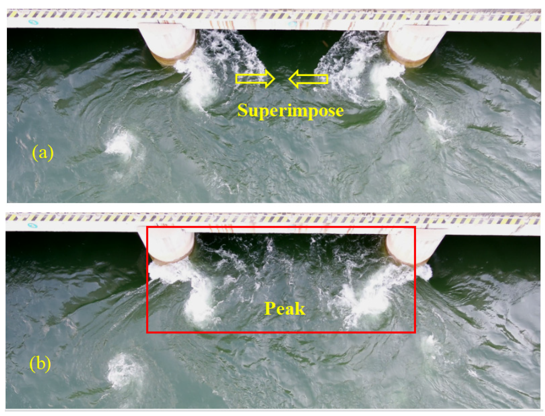
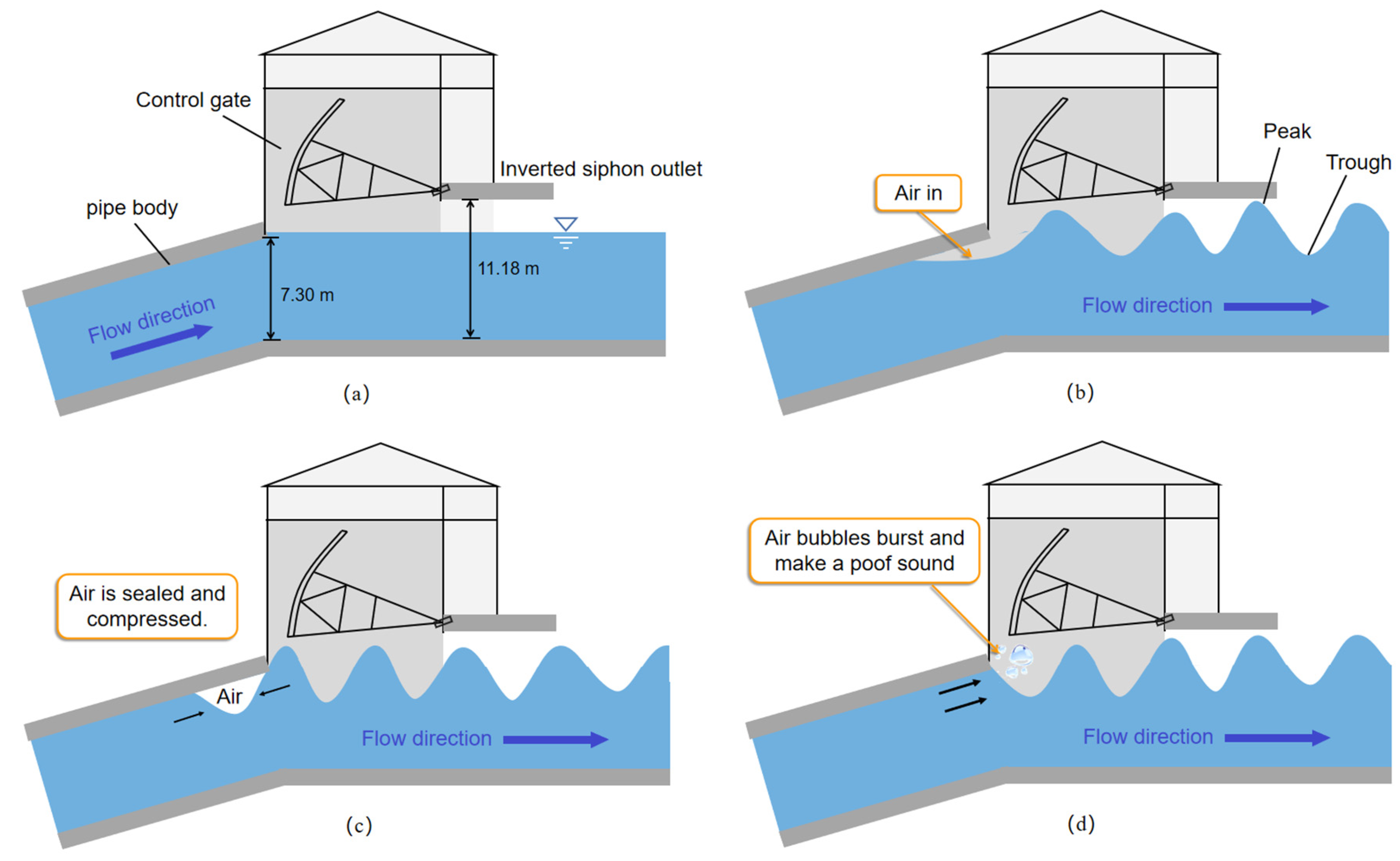
3.2. Hazards of the Karman Vortex

After analyzing the formation mechanism of the Karman vortex street, we further investigated the effect of the Karman vortex street on the flow field and building structure.
Figure 8 shows the depth distribution of the water flow. The water depth is higher in the shedding vortex area, and the most elevated position is located at the lock chamber section. The water level at the lock chambers fluctuates violently. The results show that the formation of the Karman vortex street affects the delivery capability of the gate.
We further analyzed the effect of the vortex on the water level. The time-history curves of the flow depth at the three positions (L2, M2, and R2, as shown in Figure 8) were extracted, as shown in Figure 9. Because the flow depth curves always undergo a period of change before stabilization, the calculation period of 400–1800 s was selected for analysis. It can be seen from the figure that the flow depth in the three positions rises and falls alternately, illustrating a certain fluctuation period. The fluctuation frequency and amplitude of L2 and R2 are almost the same. Due to the shedding characteristic of the Karman vortex street, the fluctuation of M2 and the side data points (L2 and R2) differ by half a cycle. When L2 and R2 appear as wave peaks, M2 just appears as wave troughs. The water level fluctuates at the same frequency as the Karman vortex shedding. Additionally, the fluctuation amplitude in M2 is significantly larger than L2 and R2, and the maximum wave amplitude in M2 reaches 0.6 m.
Figure 10 shows a fluctuation formation in the middle lock chamber. Since the vortex shedding from the two pier tails is distributed symmetrically, the vortices on both sides can diffuse to the middle lock chamber at the same time (Figure 10a). The interaction of vortex streets behind two gate piers is strengthened as vortices shed from two sides, which results in the middle lock chamber showing more substantial water-level fluctuations than those at the other two lock chambers (Figure 10b). Hence, we can conclude that the Karman vortex street significantly influences the middle outlet for the three-hole inverted siphon.
When the gates were fully opened, there was a regular “poof” sound at the inverted siphon outlet. Figure 11 shows the forming process of the “poof” sound. For the initial states, the height of the pipe body exit and the lock chamber exit were 7.3 m and 11.18 m, respectively (Figure 11a). The periodic vortex shedding makes the water surface a wavy shape at the outlet (Figure 8). It forms alternating peaks and troughs on the surface. Since the vortex is relatively close to the pipe body, the wave can be transmitted to the pipe body. The minimum flow depth at the pipe body exit reached 7.1 m (Figure 8b), which leaves the pipe exit exposed. Subsequently, the air enters the pipe (Figure 11b). As the water surface descends gradually, more air enters the inverted siphon. Before the wave’s next peak reaches the pipe exit, the air is enclosed in the pipe body. At the same time, the water coming from the rear compresses the air bubble (Figure 11c). The air bubble flows downstream under the push of the rear flow. Then, the high-pressure gas mixed with the fine stream spurts out, resulting in the “poof” sound and a surge beating the gate simultaneously (Figure 11d). Thus, the fluctuation caused by the Karman vortex shedding will affect the delivery capacity and cause abnormal noise.
The velocity distribution shown in Figure 7 shows that the vortex near the gate pier causes the velocity difference between its two sides. As a result, the gate pier is subjected to a lift force F l perpendicular to the flow direction. Here, a nondimensionalized parameter C l is defined to represent F l , which is defined as
C l = 2 F l ρ U 2 D
where C l is the lift coefficient, ρ is the fluid density, U is the average flow velocity value of 1.65 m/s at the outlet, and D is the width of the gate pier, taking the value of 1.8 m. Figure 12 shows the lift coefficient C l curves of two gate piers. The lift coefficient changes periodically, which is caused by the periodic shedding vortex at the gate pier. The periodically shedding vortices lead to constant changes in the pressure field around the pier, which leads to vibrations in the gate pier structures [36,37]. The amplitude of the left pier is about 1.7, and the amplitude of the right pier is about 1.75. In the long-term operation, the periodical lifting force will cause fatigue damage to the structure of the gate pier.

3.3. Countermeasures

According to the analysis in the previous section, the vortex shedding negatively impacts the inverted siphon structure and the flow states. Therefore, suitable countermeasures, including altering the operation mode and developing the special buildings should be implemented to suppress vortex shedding [38]. Moreover, the vortex formation and developing process can be also controlled by altering the section shape or adding appendages, such as splitter plates, fairings, and helical strakes [39,40,41]. To ensure the water delivery capacity of the inverted siphon, it is undoubtedly a better choice to optimize the design of the gate pier.
Based on the original design, we adjusted the shape of the gate pier to weaken the vortex strength. Two different styles of gate piers, a half elliptical gate pier and a trapezoidal gate pier, are suggested, as seen in Figure 13. The gate pier measures D = 1.80 m in width, and L is the length for the gate pier’s tail.
Eight simulations with elliptical and trapezoidal piers were carried out to determine the appropriate tail size of gate piers. The simulated condition of the flow rate was 263 m3/s, and L was taken as 1.8 m, 2.7 m, 3.6 m, and 5.4 m, respectively. The number of grids, boundary conditions, the flow viscosity coefficient, and the canal roughness were all set to the same values as the original pier to regulate the simulated variables. Subsequently, simulated results of different tail pier lengths are compared with the original gate pier.
The simulated results of two pier types with L = 3.6 m are shown in Figure 14. It shows that the outlet flow velocity is considerably lower than in the initial condition. The flow velocity distribution shifts from being concentrated at high velocity on one side of the gate pier to being uniform on both sides. The velocity difference between the gate pier’s leading and trailing narrows, lessening the bluff body’s flow instability. The lengthened tail reduces the adverse pressure gradient and makes the water flow converge more smoothly. It can also be found that the velocity at trapezoidal piers was slightly higher than that at elliptical piers. The vortex shedding for the trapezoidal configuration had higher intensity and contributed less to suppressing fluctuations. To further investigate the performance of the two configurations, we analyzed wave amplitudes at the lock chamber as shown in Figure 15.
Figure 15 demonstrates the effect of tail length on the fluctuation amplitudes at the middle lock chamber. Here, we define the maximum wave amplitude at the point M2 as A m . The results show that two types of piers can effectively reduce the water-level fluctuation, and the elliptical pier reduces the fluctuation amplitude more and performs better. Compared with the trapezoidal tail pier, the elliptical pier’s streamlined appearance transits the flow more smoothly. The fluctuation amplitude at the middle lock chamber with the original pier is the largest, reaching 0.6 m. With the increase of L , the vortex at the gate pier has less impact on velocity distribution, which has a better impact on controlling the vortex and less impact on the water level. The fluctuation amplitude first decreased significantly and then stabilized as L increased. When the length of the pier tail exceeds 3.6 m, the fluctuation amplitude is less than 0.13 m. Under this condition, the large fluctuation of the water level in the lock chamber is effectively controlled, and the fluctuation has little adverse effect on the water delivery capacity of the inverted siphon. When the L reaches 5.4 m, the maximum amplitude of the water level under the elliptical tail pier can be reduced to 0.11 m.
On the one hand, we confirm that the longer tail will lead to better controlled vortex shedding. On the other hand, the lengthened gate pier will also increase the frictional head loss and reduce the flow capacity. Hence, we recommend the elliptical-shaped gate pier with a 3.6 m tail length to minimize the hazards of the Karman vortex street.

4. Conclusions

Numerical investigations were carried out to study the vortex-shedding characteristics at the inverted siphon outlet with the RNG k ε turbulence model. The simulated wave height matched well with the experimental values. We found that a turbulent vortex street formed at the outlet owing to the shape of the gate pier tail. The Karman vortex obstructs the main stream, resulting in a water-level fluctuation at the lock chamber. Moreover, the vortex induces abnormal noise at the pipe body and produces an alternating force on the gate pier, adversely affecting the inverted siphon structure after long-term operation. On the other hand, the Karman vortex street has the most significant influence on the middle outlet for the three-hole inverted siphon, reducing the gate’s delivery capacity. Therefore, we propose elliptical and trapezoidal shape gate pier solutions to control the vortex shedding. The simulation results show that both types of gate piers can effectively reduce vortex strength, among which the elliptical gate pier performs better. With the increase in the length of the pier tail, the fluctuation amplitude gradually decreases. However, when the length of the gate pier tail is greater than 3.6 m, its ability to reduce the fluctuation gradually weakens. Comprehensively considering the performance, an elliptical-shaped tail with a length of 3.6 m may be taken as a proper option. It provides a reference for flow pattern optimization of other water diversion buildings.

Author Contributions

Conceptualization, X.X. and S.C.; methodology, S.C.; software, S.C. and X.M.; validation, X.M. and S.C.; formal analysis, S.C.; investigation, X.X.; resources, X.X.; data curation, S.C. and X.M.; writing—original draft preparation, S.C.; writing—review and editing, X.X. and S.C.; visualization, X.M. and S.C.; supervision, L.J.; project administration, X.X.; funding acquisition, X.X. All authors have read and agreed to the published version of the manuscript.

Funding

This research was funded by the National Natural Science Foundation of China (Grant No. 51979109), Henan Provincial Key Research, Development and Promotion Project (Grant No. 192102310015), Henan Science and Technology Innovation Talent Program (Grant No. 174200510020), and Henan Provincial University Science and Technology Innovation Team Support Program (Grant No. 19IRTSTHN030). These supports are gratefully acknowledged and greatly appreciated.

Institutional Review Board Statement

Not applicable.

Informed Consent Statement

Not applicable.

Data Availability Statement

Not applicable.

Acknowledgments

The authors of this paper would like to thank the support of China South-to-North Water Diversion Group Middle Line Co., Ltd. in completing site investigations of this study and acquiring all necessary data and information for all hydraulic simulations. The authors wish to thank all who assisted in conducting this work.

Conflicts of Interest

The authors declare no conflict of interest.

References

  1. Long, Y.; Li, Y.; Lei, X.; Hou, Y.; Guo, S.; Sun, J. A Study on Comprehensive Evaluation Methods for Coordinated Development of Water Diversion Projects Based on Advanced SWOT Analysis and Coupling Coordination Model. Sustainability 2021, 13, 13600. [Google Scholar] [CrossRef]
  2. Zhu, J.; Zhang, Z.; Lei, X.; Jing, X.; Wang, H.; Yan, P. Ecological scheduling of the middle route of south-to-north water diversion project based on a reinforcement learning model. J. Hydrol. 2021, 596, 126107. [Google Scholar] [CrossRef]
  3. Bagherian, B.; Moin, H.; Passandideh-Fard, M. Simulation of vortex shedding behind square and circular cylinders. In Proceedings of the ASME International Mechanical Engineering Congress and Exposition, Boston, MA, USA, 31 October–6 November 2008; pp. 367–373. [Google Scholar]
  4. Labbe, D.F.L.; Wilson, P.A. A numerical investigation of the effects of the spanwise length on the 3-D wake of a circular cylinder. J. Fluids Struct. 2007, 23, 1168–1188. [Google Scholar] [CrossRef]
  5. Milne-Thomson, L.M. Theoretical Hydrodynamics; Courier Corporation: Chelmsford, MA, USA, 1996. [Google Scholar]
  6. Griffin, O.M. A note on bluff body vortex formation. J. Fluid Mech. 1995, 284, 217–224. [Google Scholar] [CrossRef]
  7. Berger, E.; Wille, R. Periodic flow phenomena. Annu. Rev. Fluid Mech. 1972, 4, 313–340. [Google Scholar] [CrossRef]
  8. Wiliamson, C. Vortex dynamics in the cylinder wake. Annu. Rev. Fluid Mech. 1996, 28, 477–539. [Google Scholar] [CrossRef]
  9. Li, Z.; Jaiman, R.K.; Khoo, B.C. Coupled dynamics of vortex-induced vibration and stationary wall at low Reynolds number. Phys. Fluids 2017, 29, 093601. [Google Scholar] [CrossRef]
  10. Cao, Y.; Tamura, T.; Kawai, H. Spanwise resolution requirements for the simulation of high-Reynolds-number flows past a square cylinder. Comput. Fluids 2020, 196, 104320. [Google Scholar] [CrossRef]
  11. Qu, L.X.; Norberg, C.; Davidson, L.; Peng, S.H.; Wang, F.J. Quantitative numerical analysis of flow past a circular cylinder at Reynolds number between 50 and 200. J. Fluids Struct. 2013, 39, 347–370. [Google Scholar] [CrossRef] [Green Version]
  12. Saeedi, M.; LePoudre, P.P.; Wang, B.-C. Direct numerical simulation of turbulent wake behind a surface-mounted square cylinder. J. Fluids Struct. 2014, 51, 20–39. [Google Scholar] [CrossRef]
  13. Sattari, P.; Bourgeois, J.A.; Martinuzzi, R.J. On the vortex dynamics in the wake of a finite surface-mounted square cylinder. Exp. Fluids 2012, 52, 1149–1167. [Google Scholar] [CrossRef]
  14. Gerrard, J. The wakes of cylindrical bluff bodies at low Reynolds number. Philos. Trans. R. Soc. Lond. Ser. A Math. Phys. Sci. 1978, 288, 351–382. [Google Scholar]
  15. Wang, J.; Zheng, H.; Tian, Z. Numerical simulation with a TVD-FVM method for circular cylinder wake control by a fairing. J. Fluids Struct. 2015, 57, 15–31. [Google Scholar] [CrossRef]
  16. Wang, C.-H.; Wang, W.; Hou, D.-M.; Wang, Z.-X.; Tian, F.-Y. Abnormal Water Waves in Large-scale Conveyance Aqueduct: Causes and Countermeasures. J. Yangtze River Sci. Res. Inst. 2021, 38, 46. [Google Scholar]
  17. Aghaee-Shalmani, Y.; Hakimzadeh, H. Large eddy simulation of flow around semi-conical piers vertically mounted on the bed. Environ. Fluid Mech. 2022, 22, 1211–1232. [Google Scholar] [CrossRef]
  18. Park, I.H.; Cho, Y.J.; Lee, J.S. Analysis of Empirical Constant of Eddy Viscosity by k-ε and RNG k-ε Turbulence Model in Wake Simulation. J. Korean Soc. Mar. Environ. Saf. 2019, 25, 344–353. [Google Scholar] [CrossRef]
  19. Catano-Lopera, Y.A.; Landy, B.J.; Garcia, M.H. Unstable flow structure around partially buried objects on a simulated river bed. J. Hydroinformatics 2017, 19, 31–46. [Google Scholar] [CrossRef]
  20. Liu, M.M.; Wang, H.C.; Tang, G.Q.; Shao, F.F.; Jin, X. Investigation of local scour around two vertical piles by using numerical method. Ocean. Eng. 2022, 244, 110405. [Google Scholar] [CrossRef]
  21. Quezada, M.; Tamburrino, A.; Nino, Y. Numerical simulation of scour around circular piles due to unsteady currents and oscillatory flows. Eng. Appl. Comput. Fluid Mech. 2018, 12, 354–374. [Google Scholar] [CrossRef] [Green Version]
  22. Kocaman, S. Prediction of backwater profiles due to bridges in a compound channel using CFD. Adv. Mech. Eng. 2014, 6, 905217. [Google Scholar] [CrossRef]
  23. Younis, B.; Przulj, V. Computation of turbulent vortex shedding. Comput. Mech. 2006, 37, 408–425. [Google Scholar] [CrossRef]
  24. Schmitt, F. About boussinesq’s turbulent viscosity hypothesis: Historical remarks and a direct evaluation of its validity. Comptes Rendus Mec. 2007, 335, 617–627. [Google Scholar] [CrossRef]
  25. Ghaderi, A.; Dasineh, M.; Abbasi, S.; Abraham, J. Investigation of trapezoidal sharp-crested side weir discharge coefficients under subcritical flow regimes using CFD. Appl. Water Sci. 2020, 10, 31. [Google Scholar] [CrossRef] [Green Version]
  26. Guo, G.; Zhang, R.; Yu, H. Evaluation of different turbulence models on simulation of gas-liquid transient flow in a liquid-ring vacuum pump. Vacuum 2020, 180, 109586. [Google Scholar] [CrossRef]
  27. Yakhot, V.; Orszag, S.; Thangam, S.; Gatski, T.; Speziale, C. Development of turbulence models for shear flows by a double expansion technique. Phys. Fluids A Fluid Dyn. 1992, 4, 1510–1520. [Google Scholar] [CrossRef] [Green Version]
  28. Lateb, M.; Masson, C.; Stathopoulos, T.; Bédard, C. Comparison of various types of k–ε models for pollutant emissions around a two-building configuration. J. Wind. Eng. Ind. Aerodyn. 2013, 115, 9–21. [Google Scholar] [CrossRef] [Green Version]
  29. Yakhot, V.; Smith, L.M. The renormalization group, the ɛ-expansion and derivation of turbulence models. J. Sci. Comput. 1992, 7, 35–61. [Google Scholar] [CrossRef]
  30. Escue, A.; Cui, J. Comparison of turbulence models in simulating swirling pipe flows. Appl. Math. Model. 2010, 34, 2840–2849. [Google Scholar] [CrossRef]
  31. Li, X.-W.; Fan, J.-F. A stencil-like volume of fluid (VOF) method for tracking free interface. Appl. Math. Mech. 2008, 29, 881–888. [Google Scholar] [CrossRef]
  32. Hirt, C.W.; Nichols, B.D. Volume of fluid (VOF) method for the dynamics of free boundaries. J. Comput. Phys. 1981, 39, 201–225. [Google Scholar] [CrossRef]
  33. Zhan, J.-M.; Yu, L.-H.; Li, C.-W.; Li, Y.-S.; Zhou, Q.; Han, Y. A 3-D model for irregular wave propagation over partly vegetated waters. Ocean Eng. 2014, 75, 138–147. [Google Scholar] [CrossRef]
  34. Hu, J.; Wang, Z.; Chen, C.; Guo, C. Vortex shedding simulation of hydrofoils with trailing-edge truncation. Ocean Eng. 2020, 214, 107529. [Google Scholar] [CrossRef]
  35. Blevins, R.D. Flow-Induced Vibration; Van Nostrand Reinhold Co.: New York, NY, USA, 1977. [Google Scholar]
  36. Hu, J.; Wang, Z.; Zhao, W.; Sun, S.; Sun, C.; Guo, C. Numerical simulation on vortex shedding from a hydrofoil in steady flow. J. Mar. Sci. Eng. 2020, 8, 195. [Google Scholar] [CrossRef] [Green Version]
  37. Jia, L.-B.; Yin, X.-Z. Response modes of a flexible filament in the wake of a cylinder in a flowing soap film. Phys. Fluids 2009, 21, 101704. [Google Scholar] [CrossRef]
  38. Homescu, C.; Navon, I.; Li, Z. Suppression of vortex shedding for flow around a circular cylinder using optimal control. Int. J. Numer. Methods Fluids 2002, 38, 43–69. [Google Scholar] [CrossRef] [Green Version]
  39. Lockey, K.; Keller, M.; Sick, M.; Staehle, M.H.; Gehrer, A. Flow-induced vibrations at stayvanes: Experience on site and CFD simulations. Int. J. Hydropower Dams 2006, 13, 102–106. [Google Scholar]
  40. Mosallem, M. Numerical and experimental investigation of beveled trailing edge flow fields. J. Hydrodyn. Ser. B 2008, 20, 273–279. [Google Scholar] [CrossRef]
  41. Zobeiri, A.; Ausoni, P.; Avellan, F.; Farhat, M. How oblique trailing edge of a hydrofoil reduces the vortex-induced vibration. J. Fluids Struct. 2012, 32, 78–89. [Google Scholar] [CrossRef]
Figure 1. Calculation model of inverted siphon outlet (unit is m).
Sustainability 14 14744 g001
Figure 2. Computational domain and boundary conditions: (a) overall 3D view, (b) side view with sidewall boundary conditions, and (c) top view with inlet and outlet boundary conditions.
Sustainability 14 14744 g002
Figure 3. Measurement details: (a) Location of the measured points; (b) An operation diagram.
Sustainability 14 14744 g003
Figure 4. Comparison of numerical and measured results: (a) The velocity distribution; (b) The flow state at the outlet.
Sustainability 14 14744 g004
Figure 5. Validations of water depth: (a) Measured and simulated values; (b) Relative errors.
Sustainability 14 14744 g005
Figure 6. Vortex shedding behavior from the tail of gate pier.
Sustainability 14 14744 g006
Figure 7. Velocity distribution of the inverted siphon outlet:(a) At 1400 s; (b) At 1600 s.
Sustainability 14 14744 g007
Figure 8. Flow depth distribution of the inverted siphon outlet: (a) At 1400 s; (b) At 1600 s.
Sustainability 14 14744 g008
Figure 9. Variation of the flow depth in different data points: (a) At point L2; (b) At point M2; (c) At point R2.
Sustainability 14 14744 g009
Figure 10. The fluctuation formation process at the middle lock chamber: (a) vortices diffusing; (b) vortices shedding.
Sustainability 14 14744 g010
Figure 11. The formation process of the abnormal sound at the inverted siphon outlet: (a) The steady surface; (b) The fluctuating surface; (c) Air bubbles in the pier; (d) Air bubbles bursting.
Sustainability 14 14744 g011
Figure 12. Lift coefficient curves of two gate piers: (a) Left gate pier; (b) Right gate pier.
Sustainability 14 14744 g012
Figure 13. The shapes of the gate pier tail (unit is m): (a) ellipse, (b) trapezoid.
Sustainability 14 14744 g013
Figure 14. Velocity distribution with L value of 3.6 m: (a) The elliptical pier; (b) The trapezoidal pier.
Sustainability 14 14744 g014
Figure 15. Change in maximum wave amplitude with various values of length.
Sustainability 14 14744 g015
Table 1. Measured data at the inverted siphon outlet.
LocationMinimum Water Depth (m)Maximum Water Depth (m)
L17.017.24
L26.947.36
L36.997.25
M16.787.49
M26.717.56
M36.797.51
R16.937.25
R26.957.35
R36.987.28
Publisher’s Note: MDPI stays neutral with regard to jurisdictional claims in published maps and institutional affiliations.

