Greenhouse Gas Emissions from a Main Tributary of the Yangtze River, Eastern China

Abstract

Rivers and streams are recognized as potential greenhouse gas (GHGs: CO₂, CH₄, and N₂O) sources, contributing to global warming. However, GHG emissions from rivers and streams have received insufficient attention compared to other ecosystems (forests, grasslands, wetlands, etc.). In this study, dissolved GHG concentrations were measured in the Qingyijiang River, the longest tributary in the lower reaches of the Yangtze River, during two campaigns in September 2020 and April 2021. Our results showed that the Qingyijiang River was oversaturated with dissolved GHGs. The dissolved GHG concentration in the surface river water ranged from 8.70 to 67.38 μM CO₂, 0.03 to 2.06 μM CH₄, and 12.30 to 32.22 nM N₂O. The average diffusive GHG emission rates were 31.89 ± 22.23 mmol CO₂ m⁻² d⁻¹, 697.22 ± 939.82 μmol CH₄ m⁻² d⁻¹, and 18.12 ± 7.73 μmol N₂O m⁻² d⁻¹. The total emissions (CO₂-e) were CO₂ (58%) dominated, while CH₄ (38%) played a moderate role in total emissions. Temporally, average GHG concentrations and fluxes from the studied river in April were higher than those in September. The concentration and flux of CH₄ exhibited high spatial variability, similar to those in most rivers. In contrast, we found that there was no obvious spatial variability in CO₂ and N₂O concentrations but a significant difference among reaches in N₂O fluxes. We found that water temperature and flow velocity were the potential drivers for the regulating spatial variability in GHGs. However, no other observed limnological parameters were found in governing the spatial patterns of GHGs, suggesting a complex combination of factors governing GHG fluxes; thus, these inconspicuous mechanisms underscore the need for further research. Overall, our study suggests that this river acts as a minor source of GHGs relative to other rivers, and CH₄ cannot be ignored when considering aquatic carbon emissions.

1. Introduction

Rivers and streams have been recognized as active transformation sites in transforming organic matter (OM) and the surrounding territorial environments, sediments, and atmosphere when transporting to the oceans [1]. As globally significant emitters of GHGs to the atmosphere, rivers and streams play a disproportionate role in the carbon and nitrogen cycle due to their small coverage area on the planet [2,3,4]. In recent decades, estimated GHG fluxes from global rivers and streams have varied from 0.23 to 2.35 Pg C yr⁻¹ for CO₂ [1,3,5,6,7,8], 1.13 to 22.88 Tg C yr⁻¹ for CH₄ [2,9,10,11,12], and 0.19 to 0.68 Tg N yr⁻¹ for N₂O [12,13,14,15,16,17]. The large, prevailing uncertainty in estimating a GHG budget for global rivers, as reflected in the reported values, is due to the scarcity of available data related to low-order rivers [3,18], and a limited mechanistic understanding of the processes leading to GHG emissions [19].

Although rivers and streams represent key components of freshwater ecosystems, their role in regional or global C and N budgets and underlying biogeochemical processes is still unclear. Theoretically, riverine GHG production processes include the biodegradation of terrestrial and aqueous OM, respiration of phytoplankton, methanogenesis, and nitrification and denitrification (nitrifier and heterotrophic denitrification), while processes such as photosynthesis by phytoplankton, CH₄ oxidation, and excessive denitrification (reduce N₂O to N₂) result in GHG consumption [10,19,20]. Not only are the CO₂, CH₄, and N₂O escaping from river networks dependent on the balance of the aforementioned microbial production and consumption processes inside the rivers, but they are also relative to the gases imported from the catchment [21,22,23]. Thus, GHG emissions are tightly linked to the factors such as temperature, OM, redox conditions, nitrate, and ammonium that influence these production and consumption processes [10,19,20,24]. However, the relationships between GHGs and those factors are complicated on some occasions. For instance, anoxic streambed sediments are favorable for methanogenesis and denitrification [10,25], leading to CH₄ and N₂O emissions. When more nitrates were transported into anoxic sediments, denitrifying bacteria could out-compete methanogens for substrates and then reduce CH₄ emissions [26]. In a specific river, aquatic plant habitats will promote CO₂ absorption, which can offset CO₂ emission from the open water, ultimately determining the river as a carbon sink or source [27].

In addition, rivers and streams flow through varied landscapes, which may cause differences in abiotic and biotic factors in riverine environments that affect GHG production and consumption processes, and thereby impact riverine GHG fluxes [28,29,30]. A large number of studies have demonstrated that catchment land-use, including forestland, farmland, and urban areas, can influence the spatial variation in GHG concentrations and fluxes [31,32,33]. For example, Borges et al. [34] found that rivers draining agriculture (croplands and pastures) had a higher GHG flux than forested systems, which was contributing to excess nutrient and organic matter inputs. The rivers draining urbanized areas enhanced the GHG flux due to nutrient and organic carbon loads [35,36,37], or receiving external GHGs from sewage [38]. To improve estimates of GHG emissions from running water, it is important to understand the spatiotemporal patterns of GHG fluxes and their drivers in rivers and streams with different catchment environments. Moreover, assessments of CO₂, CH₄, and N₂O concentrations and fluxes simultaneously in a river system across seasons remain scarce.

To address the dearth of information on the dynamics and driving mechanisms of three major GHGs in a freshwater stream with varying catchment land uses, we examined the concentrations, fluxes, and potential drivers of CO₂, CH₄, and N₂O along a 309 km stretch of a subtropical river, the Qingyijiang River, subject to land use changes. The following hypotheses were tested: (1) there would be a notable spatial pattern of GHG emissions in varied reaches, due to the surrounding landscapes, and (2) there would be higher GHG emissions in spring than in autumn. In addition, CH₄ and N₂O emissions were converted into CO₂-equivalent emissions based on their 100 yr global warming potentials (GWPs), and the relative contribution of three gases to total CO₂-equivalents was quantified. Our results are intended to fill the knowledge gaps of GHG emissions in subtropical rivers and support the assessment of regional GHG budgets in inland freshwater systems.

2. Materials and Methods

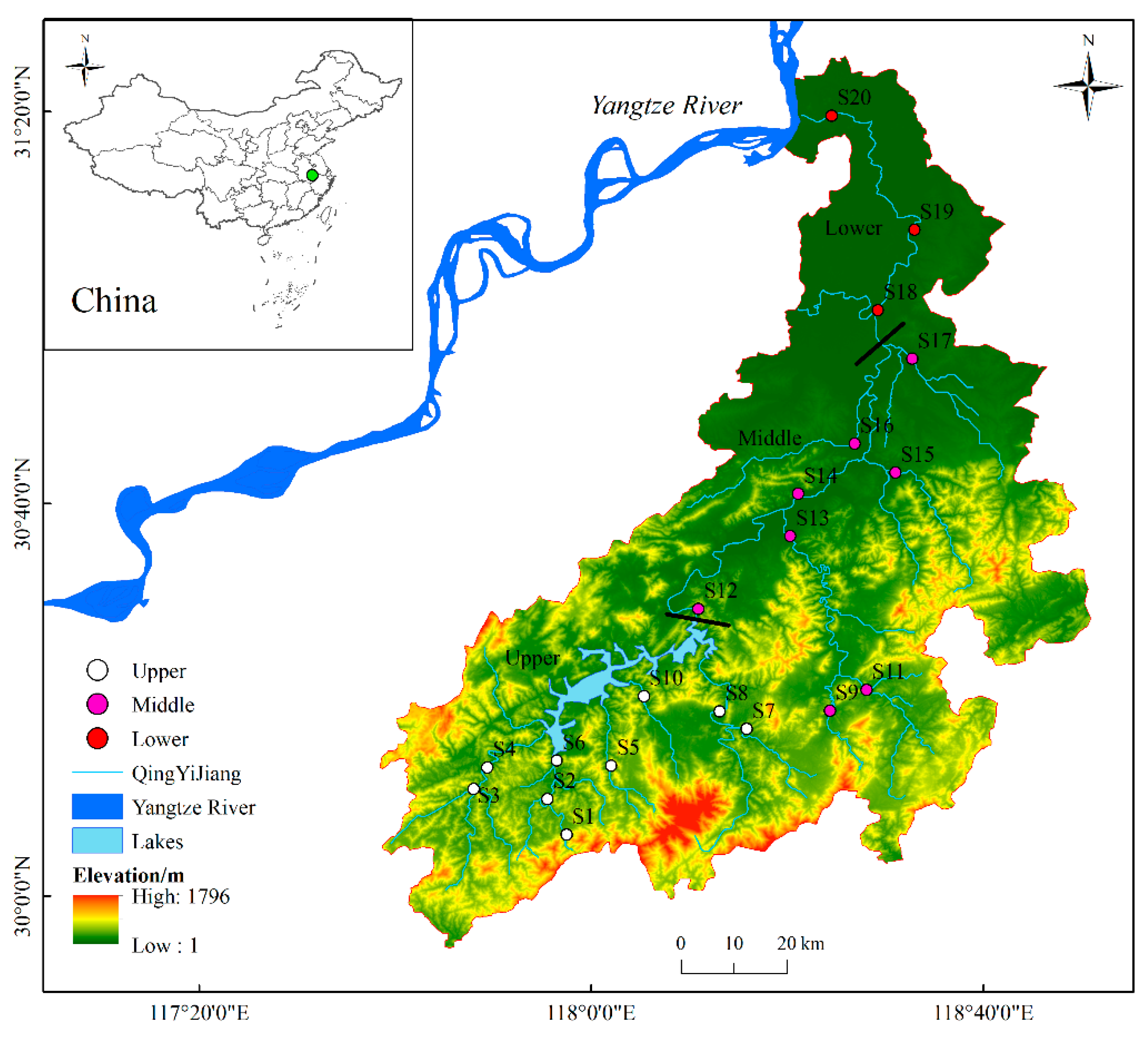
2.1. Site Description

This study was performed in the Qingyijiang catchment (29°54′ to 34°26′ N, 117°38′ to 118°51′E; Figure 1), located in the south of Anhui Province, Eastern China. The Qingyijiang River originates from the northern fringe of Huangshan Mountain and is the longest tributary in the lower reaches of the Yangtze River. The river has a length of 309 km, with a catchment area of 8487 km² and an average slope of 0.00133 m m⁻¹ [39,40]. According to a previous study, the Qingyijiang River can be divided into three parts due to its terrain differences [39]. In brief, the upper reach of the Qingyijiang River extends north from the source to the Chencun Reservoir, the middle reaches extend between the Chencun Reservoir and Wanzhi, and the lower reaches extend from Wanzhi to the outlet of the Qingyijiang River. This region is characterized by a typically subtropical monsoon climate, with a 30 yr (1981–2010) average annual temperature of 16.1 °C and average annual precipitation of 1431 mm, 71.1% of which falls from March through to September (data from http://data.cma.cn (accessed on 1 October 2022)).

The Qingyijiang River catchment is mainly overlain by Palaeozoic and Mesozoic rocks (granite, sandstone, conglomerate, limestone, shale, etc.) and Quaternary sediments (fluvial deposit, proluvial deposit, red clay, etc.) [40]. Soils are mostly red soil and yellow soil [41]. Land use types were based on an analysis of the land coverage in the catchment drainage area, which was delineated using a DEM (digital elevation model) with 4.11 m × 4.11 m resolution images obtained from Google Earth. The results showed that the Qingyijiang River catchment was occupied by forestland (63.8%), grassland (11.6%), farmland (11.6%), and unused land (8.2%). In contrast, urban land and the surface water area covered 2.7% and 2.1% of the land area in this catchment, respectively (Figure 2a). In situ measurements and water sample collections were conducted in 20 sampling sites along the Qingyijiang River during the autumn of 2020 (12–15 September 2020) and the spring of 2021 (19–20 April 2021). To explore the potential effects of land use on GHG concentrations and fluxes, the land use percentage coverage in 20 drainage segments was calculated in the buffer zone with a radius of 100 m from each sampling site.

2.2. Field Sampling and Analyses

The dissolved GHG concentration was measured by a headspace equilibration method [42]. Briefly, surface waters not exceeding 10 cm in depth were sampled by a 60 mL plastic syringe fitted with a stop-cock in triplicate, from each site. The plastic syringe was to equilibrate 40 mL of water with 20 mL of pure N₂. After vigorously shaking for 1–2 min for gas equilibrium [14,43,44], 20 mL of headspace gas was transferred to airtight TedlarR air sample bags previously flushed with pure N₂ and vacuumed. The ambient air samples were also collected in duplicate or triplicate for analysis. These gas samples were delivered to the laboratory and analyzed within 48 h.

The air temperature (Ta) was measured using a portable digital thermometer (JM 624, Jinming, China). The water temperature (Tw), dissolved oxygen (DO) concentrations, and pH were determined by a portable Multi-Parameter Water Quality Sonde (HQ40d, HACH, U.S.A.) equipped with a pH and a DO probe. The water depth (WD) was measured by a self-made sounding lead and a tape measure. Pre-acid-washed polyethylene bottles were used for storing water samples, which were collected at 10 cm below the surface. Before analysis, the bottles were maintained in cool and dark conditions. Water samples were analyzed for total phosphorous (TP) and ammonium (NH₄⁺-N) using a portable Multi-Parameter Water Quality Monitor (5B-2H, Nanbei Instrument, Zhengzhou, China) in the laboratory within 24 h. The GHG concentrations were analyzed by a modified gas chromatograph (GC-2014, Shimadzu, Kyoto, Japan) in the laboratory, which has been described in detail in Miao et al. [45].

2.3. Dissolved GHG Concentrations and Diffusive Fluxes

The dissolved GHG concentrations (c_g: CO₂ and CH₄ in μM; N₂O in nM) were calculated using Henry’s Law [42]:

c_g = p_g K_H

(1)

where the dissolved GHG concentrations are a function of the partial pressure (p_g: CO₂ and CH₄ in μatm; N₂O in natm) of the given gas in surface river water and Henry’s constant (K_H: mol L⁻¹ atm⁻¹) adjusted for ambient water temperature for the given gas. Henry’s constant K_H is usually determined by a function of the temperature and salinity [46,47,48]. Thus:

Ln K_H (CO₂) = −58.0931 + 90.5069 (100/Τ) + 22.2940 Ln (T/100) + S [(0.027766 –0.025888(T/100) + 0.0050578 (T/100)²]

(2)

Ln K_H (CH₄) = −68.8862 + 101.4956 (100/Τ) + 28.7314 Ln (T/100) + S [(−0.076146 + 0.043970 (T/100) − 0.006872 (T/100)²]

(3)

Ln K_H (N₂O) = −62.7062 + 97.3066 (100/Τ) + 24.1406 Ln (T/100) + S [(−0.058420 + 0.033193 (T/100) − 0.0051313 (T/100)²]

(4)

where T is the surface water temperature in Kelvin and S is the salinity in ‰. In this study, we assumed S = 0 in the river.

The saturation ratio (s_g) for surface-dissolved GHGs was calculated as follows:

s_g = c_g/C_eq

where C_eq is the equilibrium concentration of gas g (CO₂ and CH₄ in μM; N₂O in nM), which was calculated using the ambient atmospheric GHG partial pressure and the temperature-dependent solubility for GHGs [46,47,48]. In our study, when s_g > 1, it denotes that the water is an atmospheric GHG source; when s_g < 1, it denotes that the water is an atmospheric GHG sink.

The GHG diffusive fluxes (f_g: CO₂ in mmol m⁻² d⁻¹; N₂O and CH₄ in μmol m⁻² d⁻¹) between surface water and the atmosphere were determined by the thin boundary layer model as follows:

f_g = k_g (c_g − C_eq)

(5)

where k_g is the gas transfer velocity (cm h⁻¹). In this study, the k_g is determined by the gas transfer velocity normalized to a Schmidt number of 600 (k₆₀₀) [49]:

k_g = k₆₀₀ (SC/600)^−0.5

(6)

where SC is the dimensionless Schmidt number of a given gas. The Schmidt number SC for CO₂, CH₄, and N₂O is calculated for the surface water temperature t (°C) from the following equations [50]:

SC_CO2 = 1911.1 − 118.11 t + 3.4527 t² − 0.04132 t³

(7)

SC_CH4 = 1897.8 − 114.28 t + 3.2902 t² − 0.047608 t³

(8)

SC_N2O = 2055.6 − 137.11 t + 4.3173 t² − 0.05435 t³

(9)

k₆₀₀ is the gas transfer velocity (cm h⁻¹) normalized to a temperature of 20 °C in water with a Schmidt (SC) number of 600. Various empirical models have been developed to estimate k₆₀₀ in rivers and streams [49]. As k_g is not measured directly, the average k₆₀₀ derived from the following models was used to calculate the diffusive GHG flux for error reduction.

Using the model by Raymond et al. [49]:

k₆₀₀ = 8.42 + 11838 vS

(10)

k₆₀₀ = 3965 (vS)^0.76

(11)

k₆₀₀ = 4842 v^0.85 S^0.77

(12)

Using the model by Alin et al. [51]:

k₆₀₀ = 13.82 + 35 v

(13)

where v is the flow velocity (m s⁻¹), S is the average river slope (m m⁻¹) reported in Li [39].

2.4. Global Warming Potential (GWP)

The global warming potential (GWP) of the total GHG fluxes from the Qingyijiang River was calculated by summation of the GHG using the GWP of each gas. Over the 100-year time horizon, fluxes of CH₄ and N₂O could be converted to their CO₂ equivalents by multiplying radiative forcing factors of 30 and 273, respectively [52].

2.5. Statistical Analyses

All the data are expressed as arithmetical means ± 1 standard deviation in this study. The normality of the measured variables was examined by the Shapiro–Wilk test, and the nonnormal distributed variables were log-transformed. Differences in physical and chemical parameters, GHG concentrations, and fluxes among seasons and varied reaches were determined with one-way analysis of variance (ANOVA) with the LSD test. The coefficient of variation (CV) for GHG concentrations and fluxes was calculated by dividing the standard deviation of the variables measured on each sampling campaign by the mean value. Pearson correlation analysis was performed to explore the relationships between the dissolved GHG concentrations, diffusive GHG fluxes, and physical and chemical parameters. The statistical analyses were performed by the SPSS 22 statistical package (IBM SPSS Inc., Chicago, IL, USA).

3. Results

3.1. Variation in Stream Physical and Chemical Parameters

The characteristics of the stream’s physical and chemical parameters are shown in

Table 1. Summary of the physical and chemical variables measured in the surface water of the three river reaches during the observation period.

Month	Reaches	Ta (°C)	Tw (°C)	WD (m)	Flow Velocity (m/s)	Air Pressure (hPa)	DO (mg/L)	pH	NH4+-N (mg/L)
September	Upper	24.4 ± 1.8 a	24.3 ± 1.3 a	0.30 ± 0.21 a	0.065 ± 0.045 a	99.86 ± 0.39 b	6.32 ± 0.78	7.88 ± 0.48 a	0.13 ± 0.17 a
	Middle	24.8 ± 3.0 a	24.8 ± 0.9 a	0.26 ± 0.15 a	0.039 ± 0.030 a	100.14 ± 0.79 a	-	7.51 ± 0.19 b	0.30 ± 0.33 a
	Lower	23.0 ± 0.6 a	25.2 ± 2.2 a	0.45 ± 0.10 a	0.028 ± 0.013 a	100.73 ± 0.06 ab	-	7.56 ± 0.24 ab	0.25 ± 0.09 a
April	Upper	25.4 ± 4.3 a	20.1 ± 2.1 a	0.25 ± 0.21 a	0.048 ± 0.042 a	99.78 ± 0.63 c	8.68 ± 1.17 a	7.78 ± 0.64 a	0.12 ± 0.11 a
	Middle	28.0 ± 3.6 a	19.8 ± 2.0 a	0.29 ± 0.19 a	0.048 ± 0.023 a	100.40 ± 0.60 b	8.32 ± 0.81 a	7.96 ± 0.58 a	0.15 ± 0.12 a
	Lower	27.7 ± 2.4 a	20.3 ± 1.0 a	0.27 ± 0.09 a	0.033 ± 0.006 a	101.25 ± 0.06 a	8.65 ± 0.99 a	7.78 ± 0.23 a	0.09 ± 0.06 a
All data	Upper	24.9 ± 3.2 a	22.2 ± 2.7 a	27.9 ± 20.6 a	0.057 ± 0.043 a	99.82 ± 0.51 c	7.64 ± 1.56 a	7.83 ± 0.5 5 a	0.13 ± 0.14 a
	Middle	26.4 ± 3.6 a	22.3 ± 3.0 a	27.4 ± 16.6 a	0.044 ± 0.026 a	100.27 ± 0.69 b	7.73 ± 1.82 a	7.73 ± 0.48 a	0.23 ± 0.25 a
	Lower	25.3 ± 3.0 a	22.7 ± 3.1 a	36.2 ± 13.1 a	0.031 ± 0.009 a	100.99 ± 0.29 a	8.65 ± 0.99 a	7.67 ± 0.24 a	0.17 ± 0.11 a

Note: The different letters in a column indicate the significant difference among reaches (p < 0.05). Ta, air temperature; Tw, water temperature; WD, water depth; DO, dissolved oxygen; NH₄⁺-N, ammonium.

. The lowest surface water temperature was found in the upper reach and the highest in the lower reach in September, while the lowest surface water temperature was found in the middle reach and the highest in the upper reach. The ANOVA analysis results showed no significant difference among the reaches for water temperature (see Table S1 in the supplementary materials). The middle part of the river presented the lowest depth in September and highest depth in April. The lowest river flow velocity was found in the lower reach with an average value of 0.028 ± 0.013 in September and 0.033 ± 0.006 in April. The pH recorded in the middle reach was lower than those from the upper and lower reaches in September but higher than those from the upper and lower reaches in April. The highest average level of ammonium (NH₄⁺-N) was recorded in the middle reach, with a value of 0.30 ± 0.33 mg L⁻¹ in September and 0.15 ± 0.12 in April.

3.2. Dissolved GHG Concentrations in Surface River Water

The dissolved GHG concentrations in the surface water of the Qingyijiang River varied from 8.70 to 67.38 μM (mean: 28.17 ± 10.31 μM) for CO₂, 0.03 to 2.06 μM (mean: 0.27 ± 0.36 μM) for CH₄, and 12.30 to 32.22 nM (mean: 16.16 ± 3.16 nM) for N₂O during the observation period. The saturation ratios ranged from 0.68 to 3.33 (mean: 1.86 ± 0.57) for CO₂, from 10.49 to 752.31 (mean: 93.02 ± 130.51) for CH₄, and from 1.42 to 4.01 (mean: 1.89 ± 0.45) for N₂O.

Temporally, dissolved GHG concentrations observed in September were lower than those in April (

Table 2. Descriptive statistics of surface water GHG concentration and diffusive GHG fluxes across the water–atmosphere interface during sampling period.

Month	Reaches	cCO2 (μM)	sCO2	fCO2 (mmol m−2 d−1) #	cCH4 (μM)	sCH4	fCH4 (μmol m−2 d−1) #	cN2O (nM)	sN2O	fN2O (μmol m−2 d−1) #
September	Upper	25.50 ± 2.05 a	1.68 ± 0.09 a	29.71 ± 6.76 a (15.49 ± 9.93~43.58 ± 7.89)	0.09 ± 0.06 b	29.33 ± 16.70 b	283.84 ± 153.65 b (134.43 ± 78.22~422.07 ± 234.32)	16.08 ± 0.48 a	1.74 ± 0.11 ab	19.40 ± 2.98 a (9.95 ± 5.35~28.53 ± 3.32)
	Middle	25.82 ± 1.60 a	1.66 ± 0.09 a	25.12 ± 2.71 a (4.76 ± 6.16~41.89 ± 3.57)	0.23 ± 0.19 a	69.26 ± 55.29 a	644.76 ± 536.99 a (161.00 ± 281.30~1056.12 ± 872.91)	15.43 ± 0.49 b	1.76 ± 0.07 a	16.30 ± 2.63 b (3.36 ± 4.99~27.06 ± 2.35)
	Lower	27.91 ± 1.26 a	1.79 ± 0.24 a	28.31 ± 6.57 a (1.13 ± 0.32~49.11 ± 10.51)	0.18 ± 0.0 7 ab	54.60 ± 20.18 ab	494.17 ± 211.03 ab (18.81 ± 5.76~866.28 ± 381.03)	15.48 ± 0.51 ab	1.70 ± 0.02 b	14.60 ± 0.32 b (0.59 ± 0.12~25.44 ± 1.26)
	Overall	25.99 ± 1.89	1.69 ± 0.12	27.66 ± 5.60 (9.04 ± 9.63~43.73 ± 6.97)	0.16 ± 0.14	49.09 ± 40.59	459.76 ± 387.46 (127.72 ± 184.64~742.32 ± 641.55)	15.73 ± 0.56	1.74 ± 0.08	17.44 ± 3.15 (5.91 ± 6.01~27.48 ± 2.85)
April	Upper	29.78 ± 18.44 a	1.86 ± 0.90 a	36.00 ± 41.26 a (16.34 ± 25.55~51.65 ± 62.33)	0.37 ± 0.64 a	132.59 ± 235.67 a	973.67 ± 1694.78 a (314.38 ± 384.78~1499.93 ± 2702.71)	16.27 ± 6.29 a	1.89 ± 0.81 a	18.27 ± 14.84 a (6.54 ± 4.06~27.94 ± 23.89)
	Middle	30.64 ± 11.73 a	2.13 ± 0.73 a	35.99 ± 23.26 a (8.56 ± 8.66~61.09 ± 40.17)	0.40 ± 0.33 a	145.15 ± 115.09 a	967.45 ± 897.37 a (267.40 ± 467.51~1578.76 ± 1351.09)	17.59 ± 2.38 a	2.24 ± 0.37 a	21.04 ± 6.02 a (4.29 ± 3.86~35.71 ± 9.91)
	Lower	31.33 ± 9.89 a	2.32 ± 0.51 a	36.84 ± 16.62 a (2.13 ± 1.60~64.78 ± 29.60)	0.33 ± 0.24 a	128.12 ± 94.23 a	730.36 ± 537.08 a (41.15 ± 34.89~1278.70 ± 936.61)	14.95 ± 1.19 a	1.89 ± 0.13 a	14.46 ± 1.87 a (0.78 ± 0.46~25.38 ± 3.32)
	Overall	30.36 ± 14.30	2.04 ± 0.77	36.12 ± 30.75 (11.10 ± 18.20~57.40 ± 48.50)	0.38 ± 0.47	136.94 ± 171.03	934.69 ± 1242.65 (254.60 ± 389.81~1498.28 ± 1962.36)	16.60 ± 4.45	2.03 ± 0.60	18.81 ± 10.57 (4.78 ± 4.06~30.67 ± 17.21)
All data	Upper	27.64 ± 12.92 a	1.77 ± 0.63 a	32.86 ± 28.87 a (15.92 ± 18.81~47.61 ± 43.30)	0.23 ± 0.47 a	80.96 ± 170.56 a	628.76 ± 1220.14 a (224.40 ± 284.82~961.00 ± 1941.86)	16.17 ± 4.33 a	1.81 ± 0.56 a	18.84 ± 10.40 a (8.24 ± 4.93~28.24 ± 16.55)
	Middle	28.23 ± 8.47 a	1.90 ± 0.56 a	30.56 ± 16.95 a (6.66 ± 7.52~51.49 ± 29.28)	0.32 ± 0.28 a	107.20 ± 95.62 a	806.10 ± 733.57 a (214.20 ± 376.76~1317.44 ± 1131.50)	16.51 ± 2.00	2.00 ± 0.36 a	18.67 ± 5.11 a (3.83 ± 4.33~31.38 ± 8.27)
	Lower	29.62 ± 6.58 a	2.06 ± 0.46 a	32.58 ± 12.23 a (1.63 ± 1.17~56.95 ± 21.62)	0.26 ± 0.18 a	91.36 ± 73.05 a	612.27 ± 387.21 a (29.98 ± 649.74~1072.49 ± 678.23)	15.21 ± 0.87 a	1.80 ± 0.14 a	14.53 ± 1.20 a (0.69 ± 0.32~25.41 ± 2.25)
	Overall	28.17 ± 10.31	1.86 ± 0.57	31.89 ± 22.23 (10.07 ± 14.41~50.57 ± 34.89)	0.27 ± 0.36	93.02 ± 130.51	697.22 ± 939.82 (191.16 ± 307.84~1120.30 ± 1491.00)	16.16 ± 3.16	1.89 ± 0.45	18.12 ± 7.73 (5.34 ± 5.10~29.07 ± 12.28)

Note: The different letters in a column indicate significant differences among reaches (p < 0.05). c_CO2, c_CH4, and c_N2O represent dissolved CO₂, CH₄, and N₂O concentrations, respectively. s_CO2, s_CH4, and s_N2O represent saturations of dissolved CO₂, CH₄, and N₂O in river water, respectively. f_CO2, f_CH4, and f_N2O represent diffusive CO₂, CH₄, and N₂O fluxes, respectively. ^# The ranges of fluxes estimated by the different models are presented in the brackets.

). For all sampling sites, the average dissolved CO₂, CH₄, and N₂O concentrations in April were 16.8%, 137.5%, and 5.5%, respectively, higher than those in September.

The spatial variability in dissolved GHG concentrations was assessed by the coefficient of variation (CV) in this study. The CV values were 7.28% for dissolved CO₂ concentrations and 3.59% for dissolved N₂O concentrations in autumn, indicating that both gases were homogenously distributed, while both of them were more spatially heterogeneous than in spring (CV: 47.11% for CO₂ and 26.80% for N₂O). Compared with CO₂ and N₂O, dissolved CH₄ concentrations exhibited greater spatial variability within the river during the sampling period (CV: 85.33% in autumn and 125.14% in spring). However, the ANOVA test showed that no significant difference existed among reaches for dissolved CO₂ concentrations in either season, and for dissolved CH₄ and N₂O concentrations in spring (p > 0.05) (Table S1). The significant difference among reaches for CH₄ and N₂O only occurred in autumn. Higher dissolved N₂O concentrations were observed in the upper reaches (mean: 16.08 ± 0.48 nM) than those in the middle reaches (mean: 15.43 ± 0.49 nM), while the opposite pattern was shown for dissolved CH₄ concentrations.

3.3. Diffusive GHG Fluxes

Based on the water–air gas exchange model, the calculated diffusive GHG fluxes in the river ranged from −8.53 to 121.57 mmol CO₂ m⁻² d⁻¹, 66.94 to 5395.84 μmol CH₄ m⁻² d⁻¹, and 8.77 to 56.73 μmol N₂O m⁻² d⁻¹, as a net GHG source for the atmosphere (Table 2). The spatiotemporal patterns of diffusive GHG fluxes mimicked the spatial and seasonal variability observed in the GHG concentrations. All three gas fluxes observed in spring were higher than those in autumn, with the average fluxes of 31.89 ± 22.23 mmol CO₂ m⁻² d⁻¹, 697.22 ± 939.82 μmol CH₄ m⁻² d⁻¹, and 18.12 ± 7.73 μmol N₂O m⁻² d⁻¹. The results of the one-way ANOVA test revealed that no significant difference in GHG fluxes was observed between seasons.

The CV values of the diffusive GHG fluxes were 69.70% for CO₂, 134.80% for CH₄, and 42.64% for N₂O, and showed considerable spatial variations on the site scale throughout the sampling period. However, no significant difference in diffusive CO₂ and CH₄ fluxes was observed among the reaches in either season (p > 0.05; Table 2), while diffusive N₂O fluxes significantly differed among the reaches in the following order: upper (19.40 ± 2.98 μmol m⁻² d⁻¹) > middle (16.30 ± 2.63 μmol m⁻² d⁻¹) > lower (14.60 ± 0.32 μmol m⁻² d⁻¹) (p < 0.05; Table 2). Overall, lower CO₂ emissions and higher CH₄ and N₂O emissions were observed in the middle reach as compared to the other reaches.

The global warming potentials of CH₄ and N₂O were over the 100-year horizon, which were 30 and 273 times larger than that of CO₂, respectively [52]. For the Qingyijiang River, CH₄ and N₂O emissions would translate into 20.92 and 2.47 mmol CO₂ eq m⁻² d⁻¹, which accounted for 37.84% and 4.47% of the three GHG emissions, respectively.

3.4. Relationships between GHG Emissions and Environmental Parameters

The correlation analysis between dissolved GHG concentrations and diffusive GHG fluxes and the measured environmental parameters for each season are shown in Figure 3. In spring, there was a significant negative relationship between CO₂ concentration and flux and DO, and a significant positive relationship between CO₂ concentration and flux and TP, while we observed a significant positive relationship between CH₄ and N₂O fluxes and water temperature. In autumn, the spatial patterns of CO₂ and N₂O fluxes were significantly regulated by flow velocity. However, no significant relationship between CH₄ concentration (or flux) and the environmental variables was found in this study.

4. Discussion

4.1. Comparison of GHG Emissions with Other Rivers

A considerable number of observations in the literature have demonstrated that most of streams and rivers were supersaturated with GHGs relative to the atmosphere [3,10,19,29]. The dissolved GHG concentrations and diffusive GHG fluxes obtained from different temporal and spatial sampling strategies undertaken in the Qingyijiang River were lower than those found in most rivers and streams around the world (Table S3). However, the dissolved CO₂ and N₂O concentrations and diffusive CO₂ and N₂O flux were comparable to those reported from tropical and subtropical rivers [53,54]. Dissolved CH₄ concentrations and diffusive CH₄ fluxes were comparable to those reported from some boreal streams [24]. The lower GHG emissions in this study could be explained as follows: first, they might be associated with the low frequency of sampling measurements, which was unlikely to capture events with high GHG fluxes [55,56]. Second, they might be related to the low GHG production capacity in the studied rivers, which received less pollutant loadings compared to rivers flowing through urban regions or agriculture-dominated catchments [35,36,57]. For example, Wang et al. [58] found that the CO₂ emission from rivers in urban areas was 2–4 times higher than that in remote rural rivers. Yu et al. [35,36] and Hu et al. [54] also found higher CH₄ and N₂O fluxes from rivers draining highly urbanized landscapes. In addition, rivers draining agricultural landscapes emitted more GHGs than from natural rivers [34,57,59].

Calculating CO₂-equivalent Global Warming Potentials (GWP) on a specified year timescale enabled us to assess the relative contribution of each GHG [60]. In this study, overall CO₂-equivalent emissions for the Qingyijiang River were dominated by CO₂, which was similar to other studies [30,32,61]. It is worth noting that CH₄ and N₂O had a certain contribution to CO₂-equivalent emissions (37.84% for CH₄ and 4.47% for N₂O), which highlights the crucial role of CH₄ and N₂O in river GHG emissions.

4.2. Factors Influencing the GHG Spatial Variation

Previous studies have shown that emissions of GHGs across the river-water–atmosphere interface originate in complex microbial processes (production and consumption) in carbon and nitrogen cycles, which depend on abundant environmental parameters such as temperature, oxygen, nutrient status, and flow velocity [34,57,62]. Temperature (sediment and/or water) has been proven to be a crucial factor for determining GHG concentrations and fluxes, as a result of the influence on the microbial processes of production and consumption. Similar to studies conducted in other rivers and streams [54,57,63], a positive correlation had been found between water temperature and N₂O and CH₄ flux through Pearson correlation analysis (Figure 3), but this relationship could not be established for CO₂. A considerable number of studies have shown that microbial activity can be stimulated by suitable high water and sediment temperature, thereby affecting CH₄ and N₂O production and emission [10,63,64,65]. In addition, the solubility of CH₄ and N₂O decreases with increasing temperature; therefore, CH₄ and N₂O are immediately released into the atmosphere at high temperature [54,66]. Furthermore, temperature not only affects respiration, but also affects photosynthesis in aquatic systems [67,68]; the combined effects on CO₂ concentration may have resulted in an inconspicuous temperature dependence of CO₂ emission in this study.

Dissolved oxygen, as another important feature of habitat redox status, plays a crucial role in GHG production and consumption, thereby determining GHG concentrations and fluxes [10,19,62]. For example, CH₄ is predominantly produced via methanogenesis under low-O₂ conditions in aquatic systems [10]. However, recent studies have found that CH₄ could also be produced under an oxic environment that was originally suitable for CH₄ oxidation [69]. In this study, no significant relationship between CH₄ and DO suggests that the spatial heterogeneity of CH₄ emission could not explained by DO concentration. N₂O can be produced via N-cycling pathways such as denitrification and dissimilatory nitrate reduction to ammonia (DNRA) under anaerobic conditions, and nitrification under aerobic conditions [19]. The DO concentrations observed in the Qingyijiang River were high enough for nitrification, and the higher N₂O concentration and NH₄⁺-N concentrations were observed in the middle reach of the river, which suggests that the nitrification pathway may be an important source of N₂O. The negative relationships between DO concentration and CO₂ concentration and flux agree with previous studies for rivers [62,70] (Figure 3), and could be attributed to pelagic respiratory production of CO₂, thus decreasing DO levels.

Land use types in the catchment are important in mediating carbon and nitrogen biogeochemical processes on land, thus influencing inputs of allochthonous materials into adjacent waters [71,72,73], with the consequence of changing the magnitude of GHG fluxes [33,34]. Agricultural and urban land uses have been found to be crucial for riverine GHG production [30,34,36,37], because nutrient loadings can lead to enhanced in-stream metabolism [32]. However, the impact of land use on river GHG concentrations and fluxes can be complex, and could not be clearly observed in this study (Table S2). Although no significant correlations between GHG concentrations and fluxes and the proportions of land use were found in the present study, higher GHG concentrations were clearly observed in the group with >50% agricultural land use in both seasons (Figure 2b). This suggests the importance of agriculture in generating GHGs in the river network.

The water flow velocity is known to be an important driver in determining the spatial variability in GHG fluxes [57,62,64,74]. In the present study, the positive relationships between flow velocity and CO₂ and N₂O fluxes are consistent with a previous study [61]. The strong flow, which affected the near-surface turbulence, led to high gas transfer velocities, thus enhancing the gas evasion [49].

Although the potential drivers influencing the spatial variability in GHGs have been assessed, our findings suggest that it is difficult to predict GHG emissions from the Qingyijiang River based on existing concentration/flux-environmental parameter relationships alone.

4.3. Study Limitations and Future Research

Similar to many other studies, there exist several uncertainties associated with GHG flux estimates in the Qingyijiang River. First, the riverine GHG flux calculation was derived from the gas transfer velocity coefficient (k) and △GHG concentration (c_g − C_eq), which was associated with high uncertainty. k was computed by empirical models, rather than measured directly in the field, which makes the actual gas transfer velocity coefficients unclear. As Raymond et al. [46] compiled, there are many models with which to estimate k; however, there is no consistent principle to determine which one should be chosen. To eliminate the divergence, the average gas transfer velocity of each gas derived from the selected empirical models was applied to calculate GHG flux in this study. Despite this, future studies should determine the gas transfer velocities directly in the field in order to constrain the uncertainty in flux estimates. Secondly, our study focused on gas diffusive fluxes without considering ebullitive fluxes, which were the main emission pathway for CH₄ reported in some streams and rivers [9,55,56]. Although the studied river originates from a mountain area, the lower reaches of the river are located on a plain, where potential ebullitive fluxes may occur. Previous studies have illustrated that ebullition may contribute substantially (> 50%) to total CH₄ flux [9,55,56]; thus, this study’s estimation of CH₄ flux was conservative without considering ebullitive fluxes. Whether CH₄ is emitted through bubbles in the lower reaches of our studied river requires further study.

Finally, we also recognized that our flux estimation was biased toward sampling time and frequency. On the one hand, flux measurements conducted in the daytime may lead to bias in flux estimates, as the diel variability of GHG fluxes has been widely reported in rivers [8,75,76]. For instance, Gómez-Gener et al. [8] demonstrated that nocturnal CO₂ emissions from global streams are on average 27% greater than those estimated from diurnal concentrations alone. Chen et al. [56] found that higher CH₄ fluxes occurred during the daytime compared to the nighttime. Some researchers found that N₂O emissions from subtropical rivers during the nighttime were higher [77] or lower [78] than N₂O emissions during the daytime. These results imply that extrapolations based on daytime observations most likely result in overestimated or underestimated fluxes. On the other hand, single-time flux measurements may produce a large uncertainty in flux estimates, which has been reported for other aquatic ecosystems [79,80]. Therefore, consideration of diel variability and sampling frequency in future studies is critical to properly assess total riverine GHG fluxes.

5. Conclusions

In conclusion, here, we have investigated the spatial variability in CO₂, CH₄, and N₂O concentration and flux from a tributary of the Yangtze River located in Eastern China. Our results showed that the river was supersaturated in CO₂, CH₄, and N₂O at most of the times and at most of sites, relative to the atmosphere, but the estimated GHG fluxes were one and/or two orders of magnitude lower than those found in most rivers and streams around the world. Although the river acts as a minor GHG emitter, the crucial role of CH₄ and N₂O cannot be ignored when considering CO₂-equivalent emissions. The GHG emissions from the river varied between seasons, with the higher values appearing in spring. However, there was no significant spatial variability in CO₂ concentrations and fluxes but a significant difference among reaches in N₂O concentrations and fluxes in September. This could be explained by the varied flow velocities in the sampling sites, which determine the gas transfer velocity coefficient. Furthermore, the spatial variation in CH₄ concentration and flux was observed without obvious patterns. Unlike most studies with clear drivers for influencing the spatial variability in GHGs, we only found water temperature, DO, and flow velocity partly regulating GHG emissions, which suggests that it is difficult to predict GHG emissions from this river based on measured parameters alone. Overall, our results highlight an urgent need for more detailed studies on flux measurements to improve the reliability of riverine GHG flux estimates, and process-based measurements to help elucidate the drivers of variability in GHGs from these subtropical rivers.

References

1. Aufdenkampe, A.K.; Mayorga, E.; Raymond, P.A.; Melack, J.M.; Doney, S.C.; Alin, S.R.; Aalto, R.E.; Yoo, K. Riverine coupling of biogeochemical cycles between land, oceans, and atmosphere. Front. Ecol. Environ. 2011, 9, 53–60. [Google Scholar] [CrossRef] [Green Version]
2. Bastviken, D.; Tranvik, L.J.; Downing, J.A.; Crill, P.M.; Enrich-Prast, A. Freshwater Methane Emissions Offset the Continental Carbon Sink. Science 2011, 331, 50. [Google Scholar] [CrossRef] [PubMed] [Green Version]
3. Raymond, P.A.; Hartmann, J.; Lauerwald, R.; Sobek, S.; McDonald, C.; Hoover, M.; Butman, D.; Striegl, R.; Mayorga, E.; Humborg, C.; et al. Global carbon dioxide emissions from inland waters. Nature 2013, 503, 355–359. [Google Scholar] [CrossRef] [Green Version]
4. Marzadri, A.; Amatulli, G.; Tonina, D.; Bellin, A.; Shen, L.Q.; Allen, G.H.; Raymond, P.A. Global riverine nitrous oxide emissions: The role of small streams and large rivers. Sci. Total Environ. 2021, 776, 145148. [Google Scholar] [CrossRef] [PubMed]
5. Cole, J.; Prairie, Y.; Caraco, N.; McDowell, W.; Tranvik, L.; Striegl, R.; Duarte, C.; Kortelainen, P.; Downing, J.; Middelburg, J. Plumbing the global carbon cycle: Integrating inland waters into the terrestrial carbon budget. Ecosystems 2007, 10, 172–185. [Google Scholar] [CrossRef] [Green Version]
6. Regnier, P.; Friedlingstein, P.; Ciais, P.; Mackenzie, F.T.; Gruber, N.; Janssens, I.A.; Laruelle, G.G.; Lauerwald, R.; Luyssaert, S.; Andersson, A.J. Anthropogenic perturbation of the carbon fluxes from land to ocean. Nat. Geosci. 2013, 6, 597–607. [Google Scholar] [CrossRef] [Green Version]
7. Lauerwald, R.; Laruelle, G.G.; Hartmann, J.; Ciais, P.; Regnier, P.A.G. Spatial patterns in CO2 evasion from the global river network. Global Biogeochem. Cy. 2015, 29, 534–554. [Google Scholar] [CrossRef] [Green Version]
8. Gomez-Gener, L.; Rocher-Ros, G.; Battin, T.; Cohen, M.J.; Dalmagro, H.J.; Dinsmore, K.J.; Drake, T.W.; Duvert, C.; Enrich-Prast, A.; Horgby, A.; et al. Global carbon dioxide efflux from rivers enhanced by high nocturnal emissions. Nat. Geosci. 2021, 14, 289. [Google Scholar] [CrossRef]
9. Sawakuchi, H.O.; Bastviken, D.; Sawakuchi, A.O.; Krusche, A.V.; Ballester, M.V.R.; Richey, J.E. Methane emissions from Amazonian Rivers and their contribution to the global methane budget. Global Change Biol. 2014, 20, 2829–2840. [Google Scholar] [CrossRef] [PubMed] [Green Version]
10. Stanley, E.H.; Casson, N.J.; Christel, S.T.; Crawford, J.T.; Loken, L.C.; Oliver, S.K. The ecology of methane in streams and rivers: Patterns, controls, and global significance. Ecol. Monogr. 2016, 86, 146–171. [Google Scholar] [CrossRef]
11. Rosentreter, J.A.; Borges, A.V.; Deemer, B.R.; Holgerson, M.A.; Liu, S.; Song, C.; Melack, J.; Raymond, P.A.; Duarte, C.M.; Allen, G.H.; et al. Half of global methane emissions come from highly variable aquatic ecosystem sources. Nat. Geosci. 2021, 14, 225–230. [Google Scholar] [CrossRef]
12. Zheng, Y.; Wu, S.; Xiao, S.; Yu, K.; Fang, X.; Xia, L.; Wang, J.; Liu, S.; Freeman, C.; Zou, J. Global methane and nitrous oxide emissions from inland waters and estuaries. Global Change Biol. 2022, 28, 4713–4725. [Google Scholar] [CrossRef] [PubMed]
13. Beaulieu, J.J.; Tank, J.L.; Hamilton, S.K.; Wollheim, W.M.; Hall, R.O.; Mulholland, P.J.; Peterson, B.J.; Ashkenas, L.R.; Cooper, L.W.; Dahm, C.N.; et al. Nitrous oxide emission from denitrification in stream and river networks. Proc. Natl. Acad. Sci. USA 2011, 108, 214–219. [Google Scholar] [CrossRef] [PubMed] [Green Version]
14. Soued, C.; del Giorgio, P.A.; Maranger, R. Nitrous oxide sinks and emissions in boreal aquatic networks in Quebec. Nat. Geosci. 2016, 9, 116–120. [Google Scholar] [CrossRef]
15. Hu, M.; Chen, D.; Dahlgren, R.A. Modeling nitrous oxide emission from rivers: A global assessment. Global Change Biol. 2016, 22, 1–17. [Google Scholar] [CrossRef] [Green Version]
16. Maavara, T.; Lauerwald, R.; Laruelle, G.G.; Akbarzadeh, Z.; Bouskill, N.J.; Van Cappellen, P.; Regnier, P. Nitrous oxide emissions from inland waters: Are IPCC estimates too high? Global Change Biol. 2019, 25, 473–488. [Google Scholar] [CrossRef] [PubMed]
17. Yao, Y.; Tian, H.; Shi, H.; Pan, S.; Xu, R.; Pan, N.; Canadell, J.G. Increased global nitrous oxide emissions from streams and rivers in the Anthropocene. Nat. Clim. Chang. 2020, 10, 138–142. [Google Scholar] [CrossRef]
18. Crawford, J.T.; Striegl, R.G.; Wickland, K.P.; Dornblaser, M.M.; Stanley, E.H. Emissions of carbon dioxide and methane from a headwater stream network of interior Alaska. J. Geophys. Res. Biogeo. 2013, 118, 482–494. [Google Scholar] [CrossRef]
19. Quick, A.M.; Reeder, W.J.; Farrell, T.B.; Tonina, D.; Feris, K.P.; Benner, S.G. Nitrous oxide from streams and rivers: A review of primary biogeochemical pathways and environmental variables. Earth Sci. Rev. 2019, 191, 224–262. [Google Scholar] [CrossRef]
20. Ward, N.D.; Bianchi, T.S.; Medeiros, P.M.; Seidel, M.; Richey, J.E.; Keil, R.G.; Sawakuchi, H.O. Where Carbon Goes When Water Flows: Carbon Cycling across the Aquatic Continuum. Front. Mar. Sci. 2017, 4, 7. [Google Scholar] [CrossRef]
21. Butman, D.; Raymond, P.A. Significant efflux of carbon dioxide from streams and rivers in the United States. Nat. Geosci. 2011, 4, 839–842. [Google Scholar] [CrossRef]
22. Peter, H.; Singer, G.A.; Preiler, C.; Chifflard, P.; Steniczka, G.; Battin, T.J. Scales and drivers of temporal pCO2 dynamics in an Alpine stream. J. Geophys. Res. Biogeo. 2014, 119, 1078–1091. [Google Scholar] [CrossRef]
23. Hu, M.; Li, B.; Wu, K.; Zhang, Y.; Wu, H.; Zhou, J.; Chen, D. Modeling Riverine N2O Sources, Fates, and Emission Factors in a Typical River Network of Eastern China. Environ. Sci. Technol. 2021, 55, 13356–13365. [Google Scholar] [CrossRef]
24. Farahbod, F. Simultaneous Use of Mass Transfer and Thermodynamics Equations to Estimate the Amount of Removed Greenhouse Gas from the Environment by a Stream of Water. Environ. Model. Assess 2021, 26, 779–785. [Google Scholar] [CrossRef]
25. McClain, M.E.; Boyer, E.W.; Dent, C.L.; Gergel, S.E.; Grimm, N.B.; Groffman, P.M.; Hart, S.C.; Harvey, J.W.; Johnston, C.A.; Mayorga, E.; et al. Biogeochemical Hot Spots and Hot Moments at the Interface of Terrestrial and Aquatic Ecosystems. Ecosystems 2003, 6, 301–312. [Google Scholar] [CrossRef]
26. McCrackin, M.L.; Elser, J.J. Greenhouse gas dynamics in lakes receiving atmospheric nitrogen deposition. Global Biogeochem. Cy. 2011, 25, GB4005. [Google Scholar] [CrossRef] [Green Version]
27. Oliveira Junior, E.S.; van Bergen, T.J.H.M.; Nauta, J.; Budiša, A.; Aben, R.C.H.; Weideveld, S.T.J.; de Souza, C.A.; Muniz, C.C.; Roelofs, J.; Lamers, L.P.M.; et al. Water Hyacinth’s Effect on Greenhouse Gas Fluxes: A Field Study in a Wide Variety of Tropical Water Bodies. Ecosystems 2021, 24, 988–1004. [Google Scholar] [CrossRef]
28. Bodmer, P.; Heinz, M.; Pusch, M.; Singer, G.; Premke, K. Carbon dynamics and their link to dissolved organic matter quality across contrasting stream ecosystems. Sci. Total Environ. 2016, 553, 574–586. [Google Scholar] [CrossRef]
29. Luo, J.C.; Li, S.Y.; Ni, M.F.; Zhang, J. Large spatiotemporal shifts of CO2 partial pressure and CO2 degassing in a monsoonal headwater stream. J. Hydrol. 2019, 579, 124135. [Google Scholar] [CrossRef]
30. Andrews, L.F.; Wadnerkar, P.D.; White, S.A.; Chen, X.; Correa, R.E.; Jeffrey, L.C.; Santos, I.R. Hydrological, geochemical and land use drivers of greenhouse gas dynamics in eleven sub-tropical streams. Aquat. Sci. 2021, 83, 40. [Google Scholar] [CrossRef]
31. Mwanake, R.M.; Gettel, G.M.; Aho, K.S.; Namwaya, D.W.; Masese, F.O.; Butterbach-Bahl, K.; Raymond, P.A. Land Use, Not Stream Order, Controls N2O Concentration and Flux in the Upper Mara River Basin, Kenya. J. Geophys. Res. Biogeo. 2019, 124, 3491–3506. [Google Scholar] [CrossRef] [Green Version]
32. Galantini, L.; Lapierre, J.-F.; Maranger, R. How Are Greenhouse Gases Coupled Across Seasons in a Large Temperate River with Differential Land Use? Ecosystems 2021, 24, 2007–2027. [Google Scholar] [CrossRef]
33. Herreid, A.M.; Wymore, A.S.; Varner, R.K.; Potter, J.D.; McDowell, W.H. Divergent Controls on Stream Greenhouse Gas Concentrations Across a Land-Use Gradient. Ecosystems 2021, 24, 1299–1316. [Google Scholar] [CrossRef]
34. Borges, A.V.; Darchambeau, F.; Lambert, T.; Bouillon, S.; Morana, C.; Brouyère, S.; Hakoun, V.; Jurado, A.; Tseng, H.C.; Descy, J.P.; et al. Effects of agricultural land use on fluvial carbon dioxide, methane and nitrous oxide concentrations in a large European river, the Meuse (Belgium). Sci. Total Environ. 2018, 610–611, 342–355. [Google Scholar] [CrossRef] [Green Version]
35. Yu, Z.J.; Deng, H.G.; Wang, D.Q.; Ye, M.W.; Tan, Y.J.; Li, Y.J.; Chen, Z.L.; Xu, S.Y. Nitrous oxide emissions in the Shanghai river network: Implications for the effects of urban sewage and IPCC methodology. Global Change Biol. 2013, 19, 2999–3010. [Google Scholar] [CrossRef]
36. Yu, Z.; Wang, D.; Li, Y.; Deng, H.; Hu, B.; Ye, M.; Zhou, X.; Da, L.; Chen, Z.; Xu, S. Carbon dioxide and methane dynamics in a human-dominated lowland coastal river network (Shanghai, China). J. Geophys. Res.Biogeo. 2018, 122, 1738–1758. [Google Scholar] [CrossRef] [Green Version]
37. Tang, W.; Xu, Y.J.; Ma, Y.; Maher, D.T.; Li, S. Hot spot of CH4 production and diffusive flux in rivers with high urbanization. Water Res. 2021, 204, 117624. [Google Scholar] [CrossRef]
38. Zhang, W.; Li, H.; Xiao, Q.; Li, X. Urban rivers are hotspots of riverine greenhouse gas (N2O, CH4, CO2) emissions in the mixed-landscape chaohu lake basin. Water Res. 2021, 189, 116624. [Google Scholar] [CrossRef]
39. Li, J.J. Rivers and lakes of Anhui; Changjiang Press: Wuhan, China, 2010; pp. 1–263. (In Chinese) [Google Scholar]
40. Hu, C.; Liu, S.; Hu, C.; Xu, G.; Zhou, Y. Fluvial incision by the Qingyijiang River on the northern fringe of Mt. Huangshan, eastern China: Responses to weakening of the East Asian summer monsoon. Geomorphology 2017, 299, 85–93. [Google Scholar] [CrossRef]
41. Li, Q. Red Soils in China; Science Press: Beijing, China, 1983; pp. 1–23. [Google Scholar]
42. Goldenfum, J.A. GHG Measurement Guidelines for Freshwater Reservoirs: Derived From: The UNESCO/IHA Greenhouse Gas Emissions From Freshwater Reservoirs Research Project; International Hydropower Association (IHA): London, UK, 2010; pp. 21–123. [Google Scholar]
43. Cole, J.J.; Caraco, N.F. Atmospheric exchange of carbon dioxide in a low-wind oligotrophic lake measured by the addition of SF6. Limnol. Oceanogr. 1998, 43, 647–656. [Google Scholar]
44. Bastviken, D.; Santoro, A.L.; Marotta, H.; Pinho, L.Q.; Calheiros, D.F.; Crill, P.; Enrich-Prast, A. Methane Emissions from Pantanal, South America, during the Low Water Season: Toward More Comprehensive Sampling. Environ. Sci. Technol. 2010, 44, 5450–5455. [Google Scholar] [CrossRef]
45. Miao, Y.; Meng, H.; Luo, W.; Li, B.; Luo, H.; Deng, Q.; Yao, Y.; Shi, Y.; Wu, Q.L. Large alpine deep lake as a source of greenhouse gases: A case study on Lake Fuxian in Southwestern China. Sci. Total. Environ. 2022, 838, 156059. [Google Scholar] [CrossRef]
46. Weiss, R.F. Carbon dioxide in water and seawater: The solubility of a non-ideal gas. Mar. Chem. 1974, 2, 203–215. [Google Scholar] [CrossRef]
47. Wiesenburg, D.A.; Guinasso, N.L. Equilibrium Solubilities of Methane, Carbon-Monoxide, and Hydrogen in Water and Sea-Water. J. Chem. Eng. Data 1979, 24, 356–360. [Google Scholar] [CrossRef]
48. Weiss, R.F.; Price, B.A. Nitrous oxide solubility in water and seawater. Mar. Chem. 1980, 8, 347–359. [Google Scholar] [CrossRef]
49. Raymond, P.A.; Zappa, C.J.; Butman, D.; Bott, T.L.; Potter, J.; Mulholland, P.; Laursen, A.E.; McDowell, W.H.; Newbold, D. Scaling the gas transfer velocity and hydraulic geometry in streams and small rivers. Limnol. Oceanogr. Flu. Environ. 2012, 2, 41–53. [Google Scholar] [CrossRef]
50. Wanninkhof, R. Relationship between wind speed and gas exchange over the ocean. J. Geophys. Res.Oceans 1992, 97, 7373–7382. [Google Scholar] [CrossRef]
51. Alin, S.R.; Rasera, M.; Salimon, C.I.; Richey, J.E.; Holtgrieve, G.W.; Krusche, A.V.; Snidvongs, A. Physical controls on carbon dioxide transfer velocity and flux in low-gradient river systems and implications for regional carbon budgets. J. Geophys. Res. Biogeo. 2011, 116, G01009. [Google Scholar] [CrossRef]
52. Forster, P.T.; Storelvmo, K.; Armour, W.; Collins, J.-L.; Dufresne, D.; Frame, D.J.; Lunt, T.; Mauritsen, M.D.; Palmer, M.; Watanabe, M.; et al. The Earth’s Energy Budget, Climate Feedbacks, and Climate Sensitivity. In Climate Change 2021: The Physical Science Basis. Contribution of Working Group I to the Sixth Assessment Report of the Intergovernmental Panel on Climate Change; Masson-Delmotte, V.P., Zhai, A., Pirani, S.L., Connors, C., Péan, S., Berger, N., Caud, Y., Chen, L., Goldfarb, M.I., Gomis, M., et al., Eds.; Cambridge University Press: Cambridge, UK; New York, NY, USA, 2021; pp. 923–1054. [Google Scholar]
53. Panneer Selvam, B.; Natchimuthu, S.; Arunachalam, L.; Bastviken, D. Methane and carbon dioxide emissions from inland waters in India—Implications for large scale greenhouse gas balances. Global Change Biol. 2014, 20, 3397–3407. [Google Scholar] [CrossRef] [Green Version]
54. Hu, B.; Wang, D.; Zhou, J.; Meng, W.; Li, C.; Sun, Z.; Guo, X.; Wang, Z. Greenhouse gases emission from the sewage draining rivers. Sci. Total Environ. 2018, 612, 1454–1462. [Google Scholar] [CrossRef]
55. Wu, S.; Li, S.; Zou, Z.; Hu, T.; Hu, Z.; Liu, S.; Zou, J. High Methane Emissions Largely Attributed to Ebullitive Fluxes from a Subtropical River Draining a Rice Paddy Watershed in China. Environ. Sci. Technol. 2019, 53, 3499–3507. [Google Scholar] [CrossRef] [PubMed]
56. Chen, S.; Wang, D.; Ding, Y.; Yu, Z.; Liu, L.; Li, Y.; Yang, D.; Gao, Y.; Tian, H.; Cai, R.; et al. Ebullition Controls on CH4 Emissions in an Urban, Eutrophic River: A Potential Time-Scale Bias in Determining the Aquatic CH4 Flux. Environ. Sci. Technol. 2021, 55, 7287–7298. [Google Scholar] [CrossRef] [PubMed]
57. Xiao, Q.; Hu, Z.; Hu, C.; Islam, A.R.M.T.; Bian, H.; Chen, S.; Liu, C.; Lee, X. A highly agricultural river network in Jurong Reservoir watershed as significant CO2 and CH4 sources. Sci. Total Environ. 2021, 769, 144558. [Google Scholar] [CrossRef]
58. Wang, X.F.; He, Y.X.; Yuan, X.Z.; Chen, H.; Peng, C.H.; Zhu, Q.; Yue, J.S.; Ren, H.Q.; Deng, W.; Liu, H. pCO2 and CO2 fluxes of the metropolitan river network in relation to the urbanization of Chongqing, China. J. Geophys. Res. Biogeo. 2017, 122, 470–486. [Google Scholar] [CrossRef]
59. Audet, J.; Bastviken, D.; Bundschuh, M.; Buffam, I.; Feckler, A.; Klemedtsson, L.; Laudon, H.; Lofgren, S.; Natchimuthu, S.; Oquist, M.; et al. Forest streams are important sources for nitrous oxide emissions. Global Change Biol. 2020, 26, 629–641. [Google Scholar] [CrossRef] [Green Version]
60. Myhre, G.; Shindell, D.; Bre’on, F.-M.; Collins, W.; Fuglestvedt, J.S.; Huang, J.; Koch, D.; Lamarque, J.-F.; Lee, D.; Mendoza, B.; et al. Anthropogenic and natural radiative forcing. In Climate Change 2013: The physical Science Basis. Contribution of Working Group I to the Fifth Assessment Report of the Intergovernmental Panel on Climate Change; Stocker, T.F., Qin, D., Plattner, G.-K., Tignor, M., Allen, S.K., Boschung, J., Nauels, A., Xia, Y., Bex, V., Midgley, P.M., Eds.; Cambridge University Press: Cambridge, UK, 2013; pp. 659–740. [Google Scholar]
61. Xue, H.; Yu, R.; Zhang, Z.; Qi, Z.; Lu, X.; Liu, T.; Gao, R. Greenhouse gas emissions from the water-air interface of a grassland river: A case study of the Xilin River. Sci. Rep. 2021, 11, 2659. [Google Scholar]
62. Campeau, A.; Del Giorgio, P.A. Patterns in CH4 and CO2 concentrations across boreal rivers: Major drivers and implications for fluvial greenhouse emissions under climate change scenarios. Global Change Biol. 2014, 20, 1075–1088. [Google Scholar] [CrossRef]
63. Zhao, B.J.; Zhang, Q.F. N2O emission and its influencing factors in subtropical streams, China. Ecol. Process. 2021, 10, 54. [Google Scholar] [CrossRef]
64. Hinshaw, S.E.; Dahlgren, R.A. Dissolved Nitrous Oxide Concentrations and Fluxes from the Eutrophic San Joaquin River, California. Environ. Sci. Technol. 2013, 47, 1313–1322. [Google Scholar] [CrossRef]
65. Shelley, F.; Abdullahi, F.; Grey, J.; Trimmer, M. Microbial methane cycling in the bed of a chalk river: Oxidation has the potential to match methanogenesis enhanced by warming. Freshwater Biol. 2015, 60, 150–160. [Google Scholar] [CrossRef]
66. Miao, Y.; Huang, J.; Duan, H.; Meng, H.; Wang, Z.; Qi, T.; Wu, Q.L. Spatial and seasonal variability of nitrous oxide in a large freshwater lake in the lower reaches of the Yangtze River, China. Sci. Total Environ. 2020, 721, 137716. [Google Scholar] [CrossRef]
67. Crawford, J.T.; Stanley, E.H.; Dornblaser, M.M.; Striegl, R.G. CO2 time series patterns in contrasting headwater streams of North America. Aquat. Sci. 2017, 79, 473–486. [Google Scholar] [CrossRef]
68. Zhong, J.; Li, S.-L.; Liu, J.; Ding, H.; Sun, X.; Xu, S.; Wang, T.; Ellam, R.M.; Liu, C.-Q. Climate Variability Controls on CO2 Consumption Fluxes and Carbon Dynamics for Monsoonal Rivers: Evidence From Xijiang River, Southwest China. J. Geophys. Res. Biogeo. 2018, 123, 2553–2567. [Google Scholar] [CrossRef] [Green Version]
69. Grossart, H.-P.; Frindte, K.; Dziallas, C.; Eckert, W.; Tang, K.W. Microbial methane production in oxygenated water column of an oligotrophic lake. Proc. Natl. Acad. Sci. USA 2011, 108, 19657–19661. [Google Scholar] [CrossRef] [PubMed] [Green Version]
70. Richey, J.E.; Wissmar, R.C.; Devol, A.H.; Likens, G.E.; Eaton, J.S.; Wetzel, R.G.; Odum, W.E.; Johnson, N.M.; Loucks, O.L.; Prentki, R.T.; et al. Carbon flow in four lake ecosystems: A structural approach. Science 1978, 202, 1183–1186. [Google Scholar] [CrossRef]
71. Findlay, S.; Quinn, J.M.; Hickey, C.W.; Burrell, G.; Downes, M. Effects of land use and riparian flowpath on delivery of dissolved organic carbon to streams. Limnol. Oceanogr. 2001, 46, 345–355. [Google Scholar] [CrossRef]
72. Williams, C.J.; Frost, P.C.; Morales-Williams, A.M.; Larson, J.H.; Richardson, W.B.; Chiandet, A.S.; Xenopoulos, M.A. Human activities cause distinct dissolved organic matter composition across freshwater ecosystems. Global Change Biol. 2016, 22, 613–626. [Google Scholar] [CrossRef]
73. Lambert, T.; Bouillon, S.; Darchambeau, F.; Morana, C.; Roland, F.A.E.; Descy, J.-P.; Borges, A.V. Effects of human land use on the terrestrial and aquatic sources of fluvial organic matter in a temperate river basin (The Meuse River, Belgium). Biogeochemistry 2017, 136, 191–211. [Google Scholar] [CrossRef] [Green Version]
74. Liu, B.Y.; Tian, M.Y.; Shih, K.M.; Chan, C.N.; Yang, X.K.; Ran, L.S. Spatial and temporal variability of pCO2 and CO2 emissions from the Dong River in south China. Biogeosciences 2021, 18, 5231–5245. [Google Scholar] [CrossRef]
75. Clough, T.J.; Buckthought, L.E.; Kelliher, F.M.; Sherlock, R.R. Diurnal fluctuations of dissolved nitrous oxide (N2O) concentrations and estimates of N2O emissions from a spring-fed river: Implications for IPCC methodology. Global Change Biol. 2007, 13, 1016–1027. [Google Scholar]
76. He, B.N.; He, J.T.; Wang, J.; Li, J.; Wang, F. Characteristics of GHG flux from water-air interface along a reclaimed water intake area of the Chaobai River in Shunyi, Beijing. Atmos. Environ. 2018, 172, 102–108. [Google Scholar] [CrossRef]
77. Yang, L.B.; Yan, W.J.; Ma, P.; Wang, J.N. Seasonal and diurnal variations in N2O concentrations and fluxes from three eutrophic rivers in Southeast China. J. Geogr. Sci. 2011, 21, 820–832. [Google Scholar] [CrossRef]
78. Zhang, W.; Li, H.; Pueppke, S.G.; Pang, J. Restored riverine wetlands in a headwater stream can simultaneously behave as sinks of N2O and hotspots of CH4 production. Environ. Pollut. 2021, 284, 117114. [Google Scholar] [CrossRef] [PubMed]
79. Natchimuthu, S.; Sundgren, I.; Gålfalk, M.; Klemedtsson, L.; Bastviken, D. Spatio-temporal variability of lake pCO2 and CO2 fluxes in a hemiboreal catchment. J. Geophys. Res. Biogeosciences 2017, 122, 30–49. [Google Scholar] [CrossRef] [Green Version]
80. Wik, M.; Thornton, B.F.; Bastviken, D.; Uhlbäck, J.; Crill, P.M. Biased sampling of methane release from northern lakes: A problem for extrapolation. Geophys. Res. Lett. 2016, 43, 1256–1262. [Google Scholar] [CrossRef]
Figure 1. Geographical location of Qingyijiang River catchment and 20 sampling sites.
Sustainability 14 13729 g001
Figure 2. (a) Land use types in the Qingyijiang River catchment and (b) their percentage coverage in 20 drainage segments (circle with radius of 100 m of each sampling site).
Sustainability 14 13729 g002
Figure 3. Correlation matrix for GHG concentrations and fluxes with physiochemical parameters in the surface water of the Qingyijiang River during the measurement periods: (a) September 2020; (b) April 2021. WT, DO, AP, WD, NH4, TP, and FV represent the water temperature, dissolved oxygen, air pressure, water depth, ammonium, total phosphorous, and flow velocity, respectively.
Sustainability 14 13729 g003