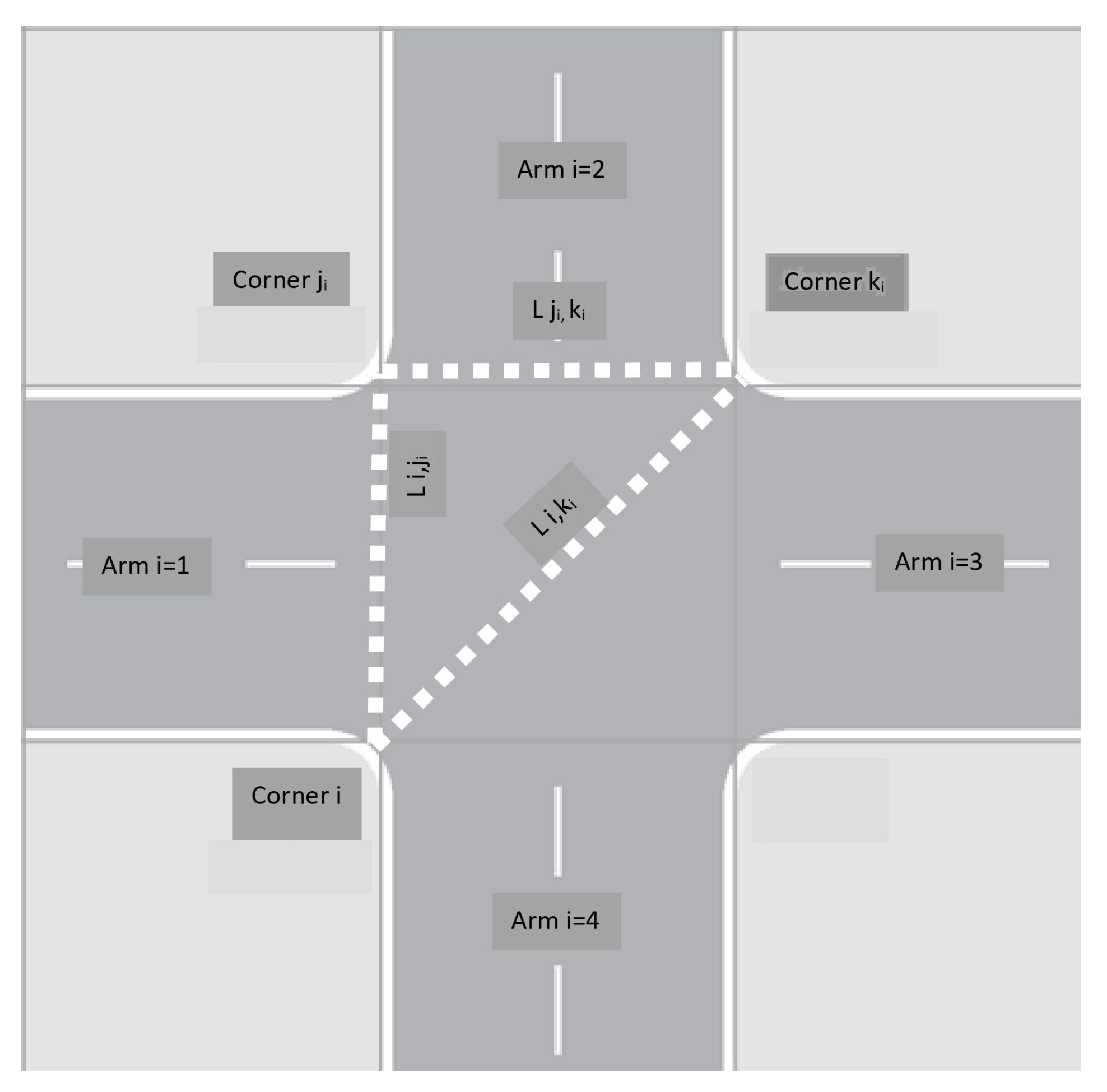
Figure 1.
Reference intersection layout with key parameters used in the simulation.
Figure 1.
Reference intersection layout with key parameters used in the simulation.
Figure 2.
Typical TWC phase diagram for a four-arm intersection.
Figure 2.
Typical TWC phase diagram for a four-arm intersection.
Figure 3.
Typical EPP phase diagram for a four-arm intersection.
Figure 3.
Typical EPP phase diagram for a four-arm intersection.
Figure 4.
Typical LTI phase diagram for a four-arm intersection.
Figure 4.
Typical LTI phase diagram for a four-arm intersection.
Figure 5.
Aerial view of the case study site–Notre-Dame and Peel intersection.
Figure 5.
Aerial view of the case study site–Notre-Dame and Peel intersection.
Figure 6.
Pedestrian and vehicle volumes during course of the day for every 15 min.
Figure 6.
Pedestrian and vehicle volumes during course of the day for every 15 min.
Figure 7.
Screenshot of the Synchro interface for the TWC pattern.
Figure 7.
Screenshot of the Synchro interface for the TWC pattern.
Figure 8.
for 80-s cycle length, with .
Figure 8.
for 80-s cycle length, with .
Figure 9.
for 80-s cycle length, with .
Figure 9.
for 80-s cycle length, with .
Figure 10.
for 80-s cycle length, with .
Figure 10.
for 80-s cycle length, with .
Figure 11.
for 60-s cycle length, with .
Figure 11.
for 60-s cycle length, with .
Figure 12.
for 60-s cycle length, with .
Figure 12.
for 60-s cycle length, with .
Figure 13.
with 60-s cycle length, with .
Figure 13.
with 60-s cycle length, with .
Figure 14.
during the day.
Figure 14.
during the day.
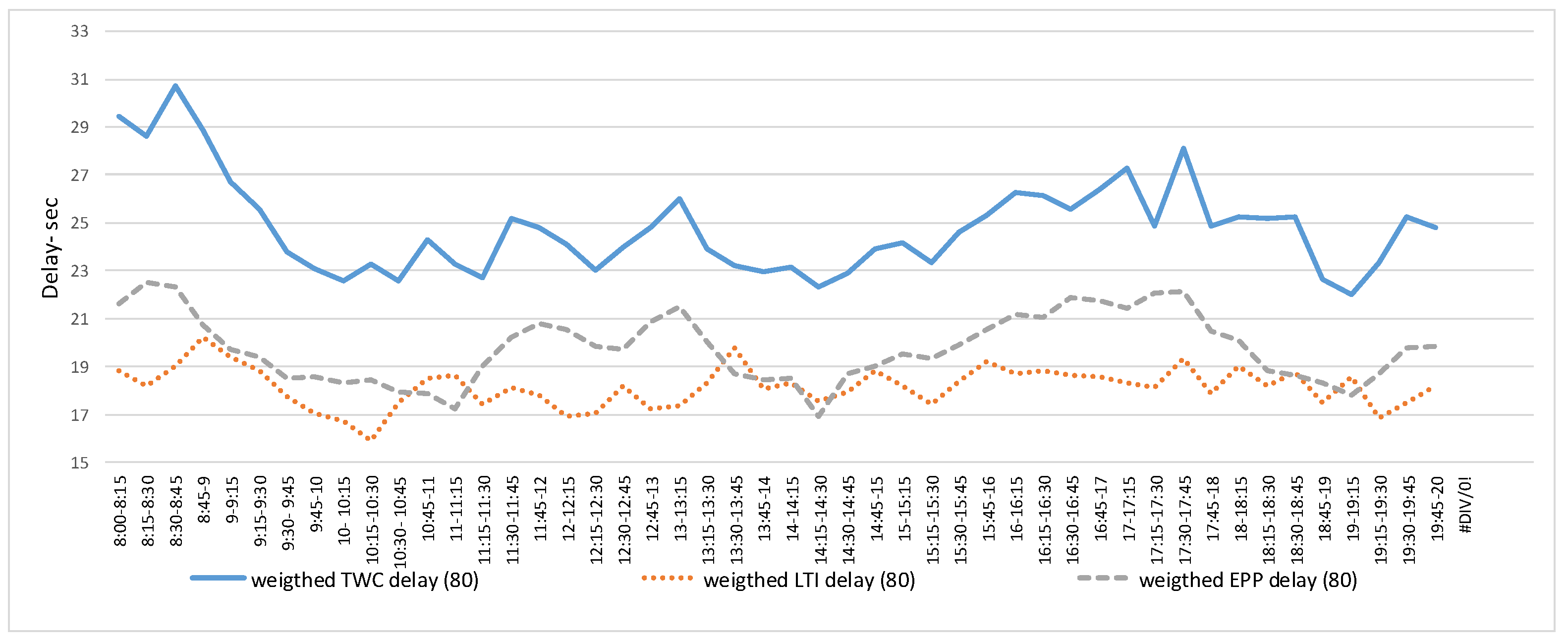
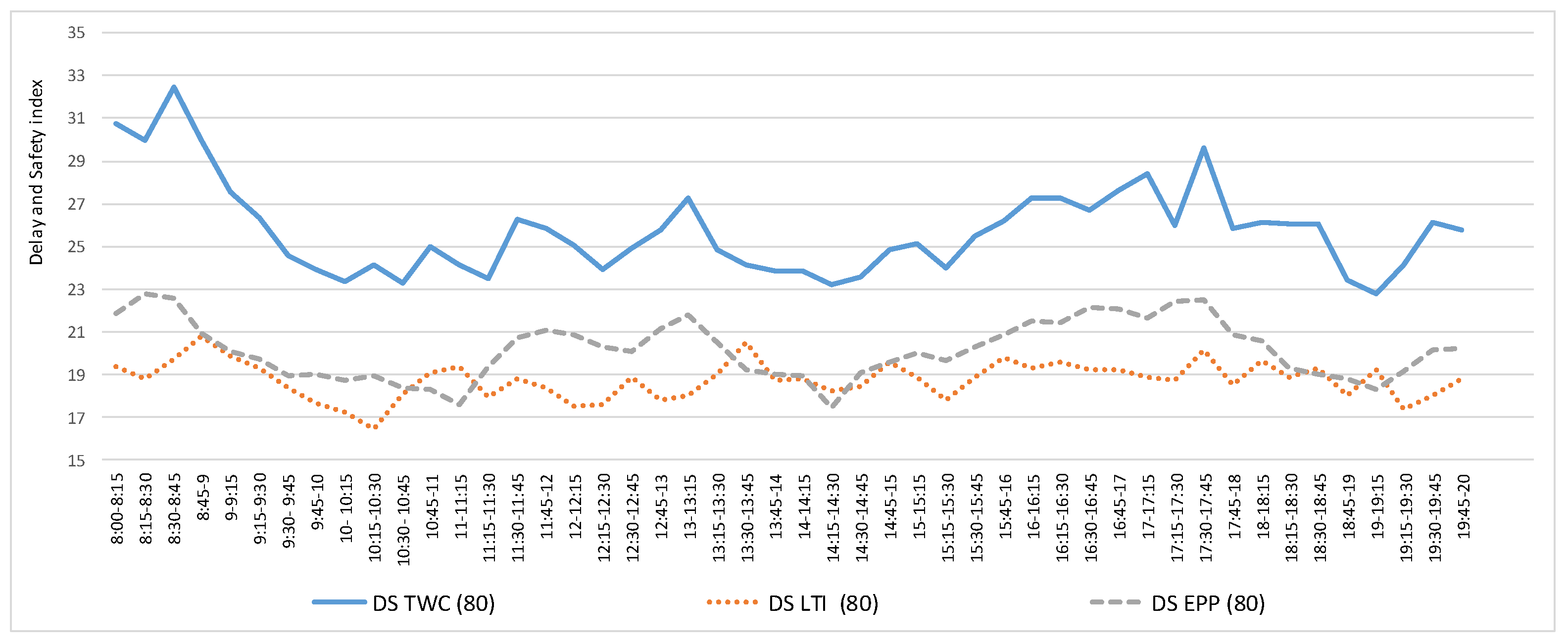
Figure 15.
for 80-s cycle length, with .
Figure 15.
for 80-s cycle length, with .
Figure 16.
for 80-s cycle length, with .
Figure 16.
for 80-s cycle length, with .
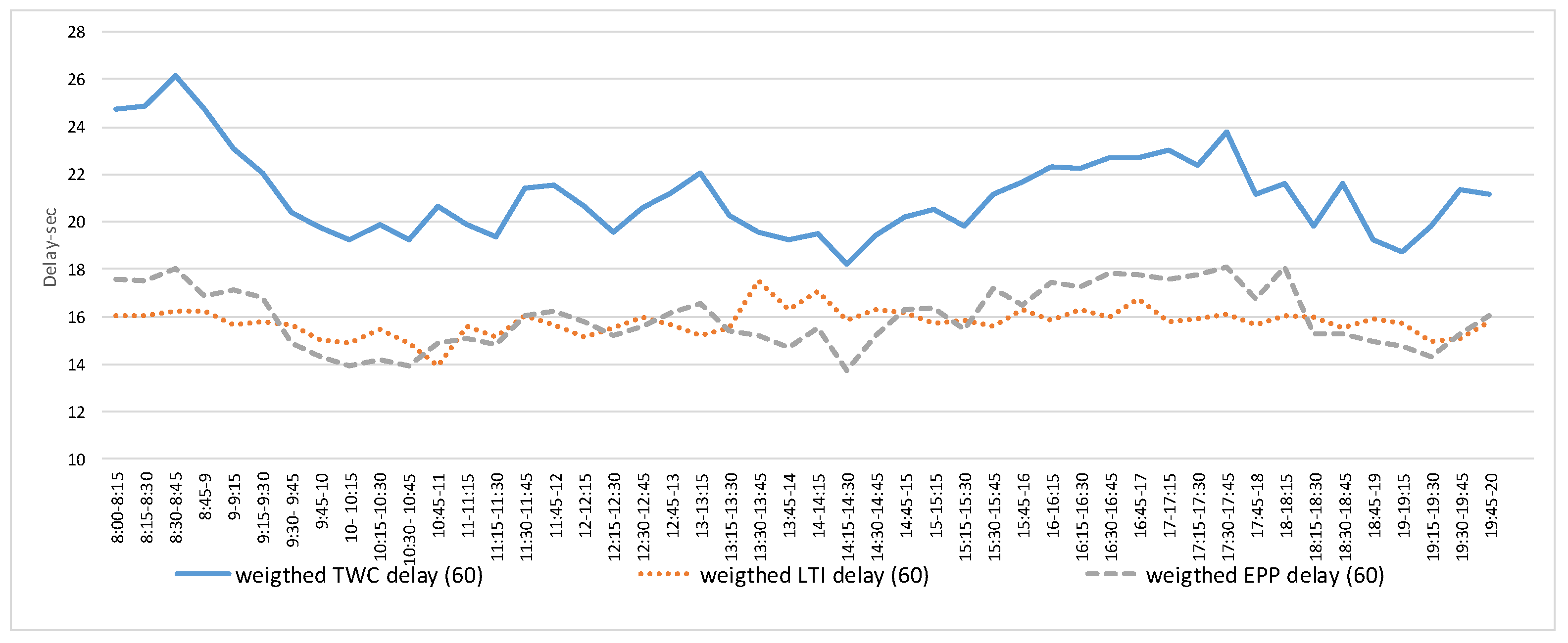
Figure 17.
for 60-s cycle length, with .
Figure 17.
for 60-s cycle length, with .
Figure 18.
for 60-s cycle length, with .
Figure 18.
for 60-s cycle length, with .
Figure 19.
for 80-s cycle length, with .
Figure 19.
for 80-s cycle length, with .
Figure 20.
for 80-s cycle length, with .
Figure 20.
for 80-s cycle length, with .
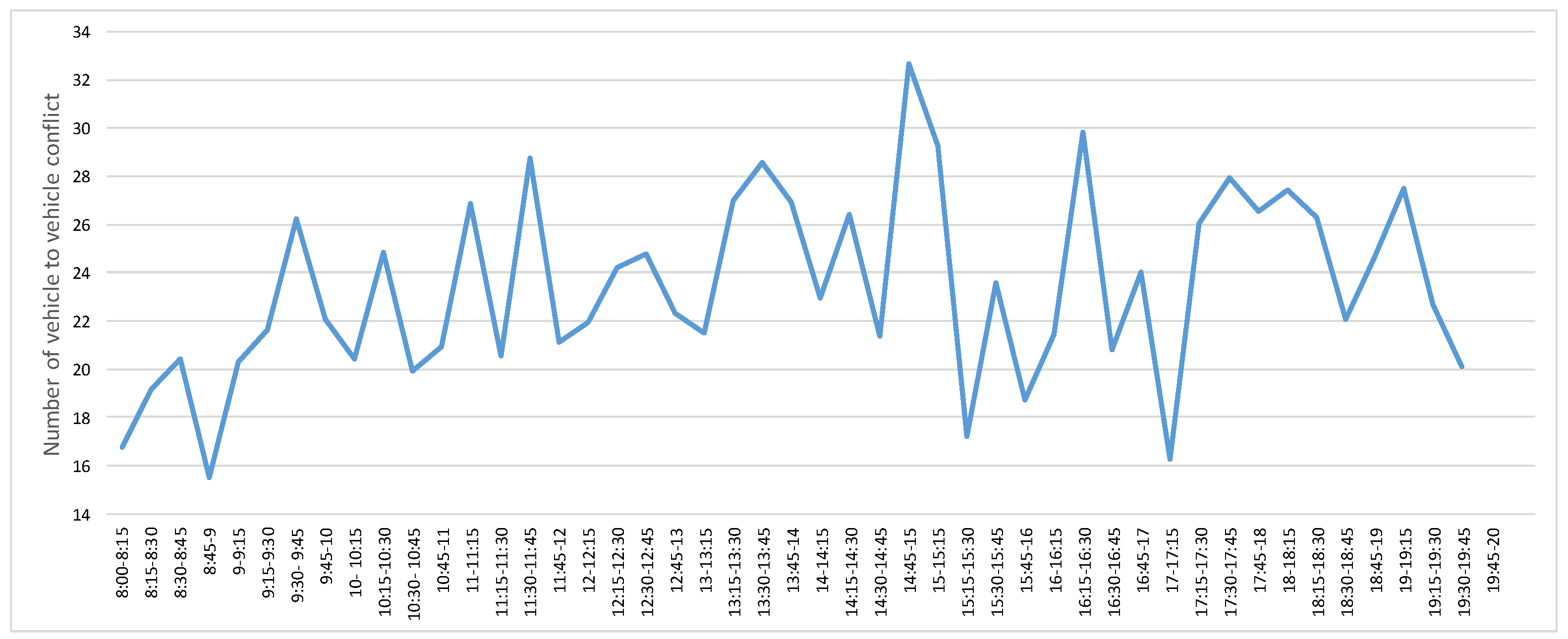
Figure 21.
comparison for 80-s cycle length, with .
Figure 21.
comparison for 80-s cycle length, with .
Figure 22.
for 60-s cycle length, with .
Figure 22.
for 60-s cycle length, with .
Figure 23.
for 60-s cycle length, with .
Figure 23.
for 60-s cycle length, with .
Figure 24.
for 60-s cycle length, with .
Figure 24.
for 60-s cycle length, with .
Figure 25.
Portion of signal pattern in 60 by varying values of .
Figure 25.
Portion of signal pattern in 60 by varying values of .
Figure 26.
Portion of signal pattern in 60 by varying values of .
Figure 26.
Portion of signal pattern in 60 by varying values of .
Figure 27.
Portion of the signal pattern in 60 by varying values of .
Figure 27.
Portion of the signal pattern in 60 by varying values of .
Table 1.
Sets, parameters and descriptions.
Table 1.
Sets, parameters and descriptions.
| Sets, Parameters, Variables | Description | Value Obtained From |
|---|
| Set of arms and corresponding corners at an intersection | – |
| Arm and corner following
| – |
| Diagonal corner from corner ,
| – |
| Duration of green for vehicles from arm , (s) | Simulation (Synchro) |
| Duration of green for pedestrian crossing arm , (s) | Simulation (Synchro) |
| Length of crosswalk from corner i to corner , (m) | Observation |
| Average walking speed of pedestrians, (m/s) | Observation |
| Portion of pedestrian volume from corner i to corner in total pedestrian demand of corner | Observation |
| t | Acceptable gap: time between vehicles when the vehicle confidently does (a) lane change(s) | Computation |
| Flow rate of vehicles turning on corner (veh/h) | Observation |
| C | Cycle length,(s) | Simulation (Synchro) |
| Pedestrian delay at intersection(s) | Computation |
| Pedestrian delay due to traffic signal at crosswalk(s) | Computation |
| Pedestrian delay due to conflicts with turning vehicles(s) | Computation |
| Number of left turning vehicles on approach during green interval of | Observation |
| Number of vehicles moving in the opposite direction on approach i during green interval of | Observation |
| Pedestrian delay due to detour distance(s) | Computation |
Table 2.
Sets, parameters, variables and descriptions.
Table 2.
Sets, parameters, variables and descriptions.
| Sets, Parameters, Variables | Description | Value Obtained From |
|---|
| Set of approaches at intersection | – |
| Number of left-turning vehicles on approach during the green interval of | Observation |
| Number of vehicles moving in the opposite direction on approach i during the green interval of | Observation |
| Probability of potential left turn conflict on approach | Computation |
| Pedestrian flow rate in the subject crossing (walking in both directions) (ped/h) | Observation |
| Pedestrian service time(s) | Simulation (Synchro) |
| Vehicle service time(s) | Simulation (Synchro) |
| Amount of permitted green time that is not blocked by (an) opposing lane(s) | Observation |
| Relevant conflict zone occupancy for conflicts between permitted or protected left-turning vehicles and pedestrians | Computation |
| Opposing demand flow rate (veh/h) | Observation |
| Effective green time for permitted left turn operation(s) | Observation |
| Critical gap(s) | Computation |
| Total vehicle volume (veh/h) | Observation |
| Total pedestrian volume (ped/h) | Observation |
| Total expected number of vehicles with potential conflicts (veh/interval) | |
| Total expected number of vehicles with potential conflicts (veh/time interval) | Computation |
| Number of left-turning vehicles with potential conflicts on approach | Computation |
| Potential conflicts of opposing vehicles resulting from left turn on approach | Computation |
| Pedestrian occupancy | Computation |
| Relevant conflict zone occupancy for conflicts between right-turning vehicles and pedestrians | Computation |
| Part of green time (g) before the first turning vehicle arrives at the intersection(s) | Observation |
| Part of the green time while left-turning vehicles stop to opposing through queue of vehicles get clear(s) | Observation |
| Portion of green time during which there is no potential conflict between left-turning and through vehicle(s) | Observation |
| Pedestrian flow rate during pedestrian service time | Computation |
| Pedestrian occupancy when the opposing queue is clear | Computation |
Table 3.
Equations related to each pattern.
Table 3.
Equations related to each pattern.
| Pattern | D (s/User) | PC (User with Conflict/Interval) | DS (s/User) |
|---|
| TWC | | | |
| EPP | | | |
| LTI | | | |
Table 4.
Hybrid improvement in comparison with the best performing pattern.
Table 4.
Hybrid improvement in comparison with the best performing pattern.
| Pattern | D (s/User) |
|---|
| LTI | 18.17 |
| 80 | 18.08 |
| Improvement | 0.49% |
Table 5.
Hybrid improvement in comparison with the best performing pattern.
Table 5.
Hybrid improvement in comparison with the best performing pattern.
| Pattern | D (s/User) |
|---|
| LTI | 15.78 |
| 60 | 15.39 |
| Improvement | 2.47% |
Table 6.
Hybrid improvement in comparison with the best performing pattern.
Table 6.
Hybrid improvement in comparison with the best performing pattern.
| Pattern | PC (Users with Conflict/15 min) |
|---|
| EPP | 23.09 |
| 80 | 23.09 |
| Improvement | 0% |
Table 7.
Hybrid improvement in comparison with the best performing pattern.
Table 7.
Hybrid improvement in comparison with the best performing pattern.
| Pattern | PC (Users with Conflict/15 min) |
|---|
| EPP | 23.09 |
| 60 | 23.09 |
| Improvement | 0% |
Table 8.
Hybrid improvement in comparison with the best performing pattern.
Table 8.
Hybrid improvement in comparison with the best performing pattern.
| Pattern | DS (s/User) |
|---|
| LTI | 18.77 |
| 80 | 18.65 |
| Improvement | 0.64% |
Table 9.
Hybrid improvement in comparison with the best performing pattern.
Table 9.
Hybrid improvement in comparison with the best performing pattern.
| Pattern | DS (s/User) |
|---|
| LTI | 16.42 |
| 60 | 15.85 |
| Improvement | 3.47% |
Table 10.
Comparison of 80-s cycle length hybrid patterns in terms of delay, conflict and .
Table 10.
Comparison of 80-s cycle length hybrid patterns in terms of delay, conflict and .
| Pattern | Unit of Measure | 80 | 80 | 80 |
|---|
| D | s/user | 18.08 | 19.83 | 18.08 |
| user with conflict/15 min | 28.98 | 23.09 | 28.96 |
| s/user | 18.90 | 20.22 | 18.65 |
Table 11.
Comparison of 60-s cycle length hybrid patterns in terms of delay, conflict and DS.
Table 11.
Comparison of 60-s cycle length hybrid patterns in terms of delay, conflict and DS.
| Pattern | Unit of Measure | 60 | 60 | 60 |
|---|
| D | s/user | 15.39 | 16.07 | 15.41 |
| user with conflict/15 min | 29.91 | 23.09 | 29.31 |
| s/user | 15.98 | 16.41 | 15.85 |
Table 12.
Improvement of hybrid patterns in comparison with best performing patterns.
Table 12.
Improvement of hybrid patterns in comparison with best performing patterns.
| Cycle Length | Percentage of Improvement |
|---|
| | |
|---|
| 80 | 0.49 | 0 | 0.58 |
| 60 | 2.47 | 0 | 3.47 |
Table 13.
Comparison of D for 60 and the best performing pattern.
Table 13.
Comparison of D for 60 and the best performing pattern.
| D for 60 | D for the Best Performing Pattern | Percentage of Improvement |
|---|
| 1 | 15.39 | 15.78 | 2.47 |
| 1.2 | 15.26 | 15.77 | 3.23 |
| 1.4 | 15.08 | 15.55 | 3.02 |
| 1.6 | 14.95 | 15.36 | 2.66 |
| 1.8 | 14.84 | 15.20 | 2.36 |
| 2 | 14.74 | 15.06 | 2.12 |
Table 14.
Comparison of for 60 and the best performing pattern.
Table 14.
Comparison of for 60 and the best performing pattern.
| DS of 60 | DS of the Best Performing Pattern | Percentage of Improvement |
|---|
| 1 | 15.85 | 16.42 | 3.47 |
| 1.2 | 17.53 | 17.96 | 2.39 |
| 1.4 | 19.42 | 19.75 | 1.67 |
| 1.6 | 21.41 | 21.72 | 1.42 |
| 1.8 | 23.55 | 23.81 | 1.09 |
| 2 | 25.73 | 26.01 | 1.07 |
Table 15.
Comparison of for 60 and the best performing pattern.
Table 15.
Comparison of for 60 and the best performing pattern.
| DS of HDS60 | DS of the Best Performing Pattern | Percentage of Improvement |
|---|
| 1 | 15.85 | 16.41 | 3.41 |
| 2 | 15.95 | 16.41 | 2.80 |
| 3 | 16.05 | 16.41 | 2.19 |
| 4 | 16.15 | 16.41 | 1.58 |
| 5 | 16.22 | 16.41 | 1.15 |
| 6 | 16.29 | 16.41 | 0.73 |


