Assessment of a Fast Proxy of Vs30 (Vs30m)

Abstract

The most frequent parameter used to quantify seismic site response in ground motion models is time-averaged shear wave velocity in the top 30 m of a site (Vs30), used by many engineering design codes and most recently by published empirical-scaling equations to estimate the amplitudes of strong ground motion. The current study explores the potential comparison of the results from the predictive equations and formula recommendations by the international building code. A total of 53 synthetic and real data models with distinct types of vs. profile were used to determine the theoretical dispersion curves and avoid forward and inverse modeling. In the prediction equation, VR36 and VR40 were employed to estimate Vs30. Furthermore, using VR40, based on the 53 different models, shows a good agreement with Vs30. The thickness of the first layer substantially affects the correlation. The findings calculated by the correlation are not in the acceptable zone for layer thicknesses of 10 < H < 20 m and thin layers at shallow depths with lower shear wave velocity.

1. Introduction

Soft surface sediments over stiff bedrock contribute to the amplification of earthquake ground motions. This amplification, combined with the vulnerability of buildings and infrastructure, may result in severe earthquake disasters. As a result, its evaluation is critical for damage mitigation in geotechnical earthquake engineering. Ground motion records, particularly at the vertical array site, have been used to evaluate site amplification, as have numerical simulations that take into account complex subsurface structures, such as the 3D basin model, and nonlinear soil behavior, such as the cyclic mobility of saturated sand [1,2]. To accurately evaluate the site amplification, detailed investigations of the subsurface structures and dynamic behavior of the target soil are required.

The time-averaged shear wave velocity over the first 30 meters, Vs30, is the most commonly used proxy for determining the dynamic behavior of soil. The shear wave velocity vs. is an essential metric in geotechnical engineering for measuring the dynamic behavior of soil. Most earthquake ground-motion prediction equations (GMPEs), site-classification studies, seismic hazard assessment, and the construction of seismic micro zonation maps employ the average shear wave velocity of the upper 30 meters of a soil profile (Vs30) as an essential metric [3,4,5,6,7,8,9].

Table 1. Classification based on VS30 for seismic codes and standard regulations from Europe, Spain, and United States.

Eurocode 8 (Europe)			NCSE-02 (Spain)			ASCE 7-16 (USA)
Soil Type	Description	VS30 (m/s)	Soil Type	Description	VS30 (m/s)	Soil Type	Description	VS30 (m/s)
A	Rock or other rock-like geological formation, including at most 5 m of weaker material at the surface.	VS > 800	I	Compact rock, very dense cemented or granular soil.	VS > 750	A	Hard Rock	VS > 1500
						B	Rock	750 < VS ≤ 1500
B	Deposits of very dense sand, gravel, or very stiff clay, at least several tens of meters in thickness, characterizes by a gradual increase of mechanical properties with depth.	360 < VS ≤ 800	II	Very fractured rock, dense or cohesive hard granular soil.	400 < VS ≤ 750	C	Very dense soil and soft rock	360 < VS ≤ 750
C	Deep deposits of dense or medium dense sand, gravel, or stiff clay with thickness from several tens to many hundreds of meters.	180 < VS ≤ 360	III	Granular soil of medium compactness or cohesive soil of firm consistency to very firm.	200 < VS ≤ 400	D	Stiff soil profile	180 < VS ≤ 360
D	Deposits of lose-to-medium cohesion- less soil or of predominantly soft-to-firm cohesive soil.	VS < 180	IV	Loose granular soil or soft cohesive soil.	VS < 200	E	Soft soil profile	VS < 180
E	A soil profile consisting of a surface alluvium layer with VS values of type C or D and thickness varying between about 5 m and 20 m, underlain by stiffer material with Vs > 800 m/s.	–	–	–	–	F	Other, see ASCE 7-16 Table 20.3-1	–
S1	Deposits consisting of or containing a layer at least 10 m thick of soft clays/silts with a high plasticity index (PI > 40) and high water content.	VS < 100	–	–	–	–	–	–
S2	Deposits of liquefiable soils, sensitive clays or any other soil profile not included in types A-E or S1	–	–	–	–	–	–	–

shows European and American seismic site categories based on the Vs30 (seismic codes and structural standards) [10,11,12,13].

Different seismic approaches, including cross hole seismic (CS), downhole seismic (DS), and surface wave approaches, can be used to determine the shear wave velocity (Vs) of the materials that are close to the surface. In the CS test, the source and receiver are positioned at equal depths within two neighboring boreholes, and the compressional wave (P-wave) and shear wave (S-wave) velocities are determined using the source-to-receiver distance and the velocities of the P- and S-waves’ respective trip periods. In the DS test, seismic waves are produced on the ground surface, the P- and S-wave travel times are measured with the receiver positioned at various depths inside a borehole, and the velocities of the P- and S-waves are then estimated using the distance between the source and receiver as well as the P- and S-wave travel times. Compared to surface wave approaches, the CS and DS methods are more reliable and exact [14,15,16]. The CS and DS methods, however, are intrusive and expensive. In the case of low cost projects, it is also not economically feasible to estimate the Vs. using the CS and DS approaches. The surface wave methods, however, are reliable, non-intrusive, affordable, and useful approaches to estimate the vs. of the near-surface materials [17,18].

In order to estimate the Vs. of the near-surface materials for seismic site assessment, surface wave methods are therefore regarded as innovative techniques by geotechnical earthquake engineers, geophysicists, and geologists.

Traditionally, Vs30 is determined by the seismic measurement in the borehole, for instance, down hole, cross-hole, or suspension logging methods. These methods are time-consuming and uneconomical. A faster, more accurate, and cost-effective method is needed to measure the Vs30 efficiently. Noninvasive surface wave methods, for instance, spectral analysis of surface waves (SASW), multichannel analysis of surface waves (MASW), and array micro tremor and refraction micro tremor techniques are proven nondestructive seismic methods that can be used to determine the variation of vs. with depth [19,20,21]. These methods are cost-effective, do not require boreholes, and are widely used for determining Vs30. The basis of surface wave methods is the dispersive characteristic of Rayleigh waves (VR) when propagating in a layered medium. These surface wave methods consist of collecting surface wave phase data in the field to determine the dispersion curve. The variation of phase velocity Vph with Rayleigh wave VR or frequency is called dispersion. The Rayleigh wave phase velocity depends on the site characteristics, for instance, shear wave velocity, compression wave velocity, density, and Poisson’s ratio. After determination of the dispersion curve by using iterative forward or inverse modeling techniques to back-calculate the corresponding vs. profile, VS30 can be calculated. Due to the non-uniqueness problem in the inversion analysis, and based on the comprehensive study, the authors of [22,23] proposed two predictive equations for the fast determination of Vs30 by using Rayleigh wave velocity at wavelengths 36 and 40 m. This predictive equation was derived by using linear regression analysis on a set of Rayleigh-wave dispersion curves and Vs30 values that were calculated from the seismic velocity profile.

This velocity profile was estimated by down hole and P-S suspension logging, and each velocity profile contained shear wave velocity and compression wave velocity.

Fifty-three real field and synthetic velocity profiles, as shown in Figure 1, were selected to verify the predictive equation. For each VS and VP profile, the fundamental-mode Rayleigh wave dispersion curve was calculated. The corresponding density for each layer was used when determining the fundamental mode dispersion curve. Reasonable variations in mass density have a negligible effect on dispersion. The evaluation of predictive equations based on different synthetic and real data velocity profiles is thoroughly discussed below.

2. Methods

The results from the predictive equations developed by [20], Equation (1), and Martin and Diehl, (2004) Equation (2), for wavelengths corresponding to the phase velocity of the Rayleigh wave at 36 m (VR36) and 40 m (VR40), respectively, were compared with the result from the formula recommended by the international building code 2000, Equation (3), for the fast determination of Vs30. We set up fifty-three simple synthetic and real data typical earth velocity profiles to determine its theoretical dispersion (model dispersion) curve. Because only one point VR36 or VR40 is needed in the dispersion, these fifty-three models are divided into three different groups. As illustrated in Figure 1, Group A consists of twenty-five synthetic two-layered earth profiles with (a) a weak, soft layer overlaying stiff soil (Figure 1a), (b) a weak, soft layer overlaying soft rock (Figure 1b), (c) a weak, soft layer overlaying rock (Figure 1c), and (d) a weak layer overlaying hard rock (Figure 1d). Group B consists of six constant gradient synthetic Earth profiles frequently encountered in the field as shown in Figure 1e. Group C consists of twenty-seven accurate data models, taken from the Puerto Rico Seismic Network [24]. As illustrated in Figure 1f. When performing modal dispersion curve analysis, the typical densities corresponding to the stiffness of each layer were used. For each Vs and Vp profile, the fundamental mode Rayleigh wave dispersion curve was determined by the famous dynamic stiffness matrix method [25]. In a layered medium, for the given velocity profile, the wave equation leads to a characteristic equation, in which for a single frequency, multiple possible roots of phase velocity (Vph) or wavelength can be found. These solutions are the model dispersion curves, in which the lowest phase velocity (Vph) and frequency are the fundamental modes, and higher phase velocity is the higher mode. Modeling was performed in the wavelength domain instead of the frequency domain.

$$Vs30=1.076\ast VR36$$

(1)

$$Vs30=1.045\ast VR40$$

(2)

$$Vs30={\displaystyle \sum di/{\displaystyle \sum ti=30/{\displaystyle \sum (di/Vsi)}}}$$

(3)

Theoretical Dispersion Curve

In most cases, theoretical dispersion curves are determined by the matrix method developed by [25] and global stiffness matrix formulations for a layered system that originated in the work of [26]. In this work, the more stable global stiffness matrix method was used to compute theoretical dispersion curves. For a horizontally layered medium, by assuming axial symmetric motion (i.e., ground motion subjected to circular vertical loading), an element stiffness matrix was obtained for each layer, including the half space. The element stiffness matrix of a given layer relates the stresses at the upper and lower interfaces of the layer to the associated displacement, which can be determined in frequency (W) and wave number (k) by the general solution of the wave equation. Similar to the finite element methods, the global stiffness matrix “K” can be determined by assembling an element stiffness matrix, corresponding to each nodal force to the nodal displacements at the layer interfaces. For a non-trivial solution, the determinate of the global stiffness matrix K(w,k) should be zero. For a constant frequency, the value of wavenumber (K), the phase velocity Vph = w/k can be determined by setting the determinant of the global stiffness matrix method equal to zero. The global stiffness matrix method is basically a root-finding method. The different wavenumbers k (or phase velocities Vph) determined at a given frequency correspond to dispersion curves with other modes. For instance, the largest wavenumber, hence the lowest phase velocity, for a frequency belongs to the fundamental mode, and the second largest wavenumber belongs to the second mode. An open-source software, MAS Waves [27] has included a function (MASWaves_theoretical_dispersion_curve.m) to compute the fundamental-mode dispersion curve in terms of wavelength vs. phase velocity, which was used in this study.

3. Result and Discussion

Our discussion concentrates on whether VR36 or VR40 should be used in the predictive equation to determine the fast proxy of Vs30 for various synthetic and real data velocity profiles. The fundamental mode of Rayleigh wave dispersion curves was calculated based on the dynamic stiffness of 53 velocity profiles. The value of Vs30 calculated by the predictive equation was compared to the actual value of Vs30 determined by the formula recommended by the international building code, as shown in Equation (3). With the exception of a few cases, the difference between the actual and predictive values of Vs30 is usually within +/− 10% error bound zone. The following results summarize the selection of a more suitable predictive equation and the evaluation of Vs30 proxy.

3.1. GROUP A

Group A consists of twenty-five two-layer synthetic earth profiles with different velocity contrasts as illustrated in Figure 1a–d. The first layer, with varying depth and constant shear wave velocity (120 m/s) and with varying half space shear velocity to a depth of 30 m, was used to calculate the fundamental mode model dispersion curve based on the dynamic stiffness matrix method. The following discussion summarizes the selection of VR 36 or VR 40 in the predictive equation for determining Vs30.

3.1.1. Weak Soil Layer Overlaying Stiff Soil

Figure 1a shows the two-layer constant velocity profile with varying depth of the first layer. Due to the low-velocity contrast, overall, the actual Vs30 has good correlation with the Vs30 determined by the predictive equation, and it lies within the +/−10% error bound zone, but the Vs30 calculated using VR40 in the predictive equation is closely related to the actual Vs30, as shown in Figure 2. Both results are underestimated by using VR36 and VR40 at a height of 15 m (H15 top layer height) and 20 m (H20).

3.1.2. Weak Soil Layer Overlying Soft Rock

Similar to Figure 1a, Figure 1b represents the weak soil overlaying the soft rock. The correlation results between the Vs30 and Rayleigh wave phase velocities (VR36, VR40) lead to a similar conclusion. At the heights of 5 and 25 m, Vs30 is determined by using VR36 and VR40 in the predictive equations. The result of Vs30 is within +/−10% error bound zones. At the height of 10 m, VR40 is within +/−10% error bound zones, while VR36 is not in an acceptable zone. Similarly, at 15 and 20 m, the Vs30 determined by using VR36 is underestimated. Overall, VR40 shows an appropriate agreement with actual Vs30, as illustrated in Figure 3.

3.1.3. Weak Layer Overlaying Rock

Figure 1c represents the case of a weak layer over rock. The results show that Vs30 calculated by the predictive equations was underestimated due to a high-velocity contrast, and the correlation between Vs30 and VR at a wavelength of 36 and 40 m is not in a reasonable range. The results are basically dominated by using VR50 in the predictive equation, as shown in Figure 4.

3.1.4. Weak Layer Overlaying on Hard Rock

Similar to the other two-layer velocity profile, the velocity of the first layer was kept constant with variable height, as shown in Figure 1d. Due to the high-velocity contrast between the two layers, it is clear from the results that Vs30 was calculated by the predictive equation using the Rayleigh wave velocity at VR36, VR40 is not promising, and not one data point lies within the +/−10% acceptable error bound zone. Vs30 was estimated by using VR50. Two velocity profiles, for instance, H20 and H25, are within +/−10% error bound zone, as shown in Figure 5.

3.2. Synthetic Data Representation

This approach summarizes the synthetic data representation, as illustrated in Figure 6, and it is the most sophisticated correlation to obtain an information about the selection of the Rayleigh wave velocity at a specific wavelength, for instance, VR36, VR40, and VR50, to use in the predictive equations for the calculation of Vs30 within the acceptable +/−10% error bound zone. The green, blue and red circles represent the upper boundary of the phase velocity of the Rayleigh wave at wavelengths of 36, 40 and 50 m, respectively. Bold black circles represent the two-layer synthetic models as discussed above. The colored zone shows the correlation between Vs30 and VR at wavelengths of 36, 40 and 50 m with an error of +/−10%, which is an acceptable zone. The Rayleigh wave velocity at a wavelength of 50 m, i.e., VR50, covered more area for high-velocity contrast than VR40 and VR36. The velocity contrast was not significantly higher between the first layer and the half space, as shown in Figure 1a, with a first layer thickness of 22 m < H < 13 m, and Vs30 was determined by the predictive equation by using the Rayleigh wave velocity at a wavelength of VR36, which lies within the acceptable zone. In this case, by using VR40, the Vs30 lies within the acceptable zone, as shown by a dark black circle on the VR40 line. In the case of a weak layer over soft rock, the Vs30 calculated by the predictive equation by using VR36 and VR40 lies in the acceptable error bound zone only if the thickness of the first layer lies between 22 m < H < 10 m and 20 m < H < 10 m. However, VR50 will be in the acceptable zone. As the velocity contrast between the top layer and the half space becomes more significant, as shown in Figure 1c, by using VR40 and VR50, Vs30 will be in an acceptable zone if the height of the first layer is between H > 22 m and 5 m > H > 10 m. Due to a very high velocity contrast, Vs30 calculated by VR50 lies within the acceptable zone, as shown in the figure below, for weak soil over hard rock.

3.3. Group B Synthetic Gradient Models

At many sites, under typical geological conditions, soil stiffness increases gradually with depth due to its geological age, cementation, compaction, overburden pressures, etc., and the effect of the non-fundamental mode Rayleigh wave energy on the dispersion curve is minimal. In this situation, the common expectation includes engineering fill over stiff sediments, asphalt, concrete, and soft loose material on the compacted base materials or soft soil over shallow soft rock. To represent these conditions in the field, six gradient synthetic models were selected as illustrated in Figure 1e to calculate its theoretical dispersion curves. Vs30 was determined by the predictive equations using VR36, VR40 and VR50. From the results as shown in Figure 7, it was concluded that Vs30 has a very good correlation with the phase velocity of the Rayleigh wave at a wavelength of 36 m, i.e., VR36. All the data points are in the acceptable zones. The Vs30 calculated by using VR40 and VR50 in the predictive equation was overestimated.

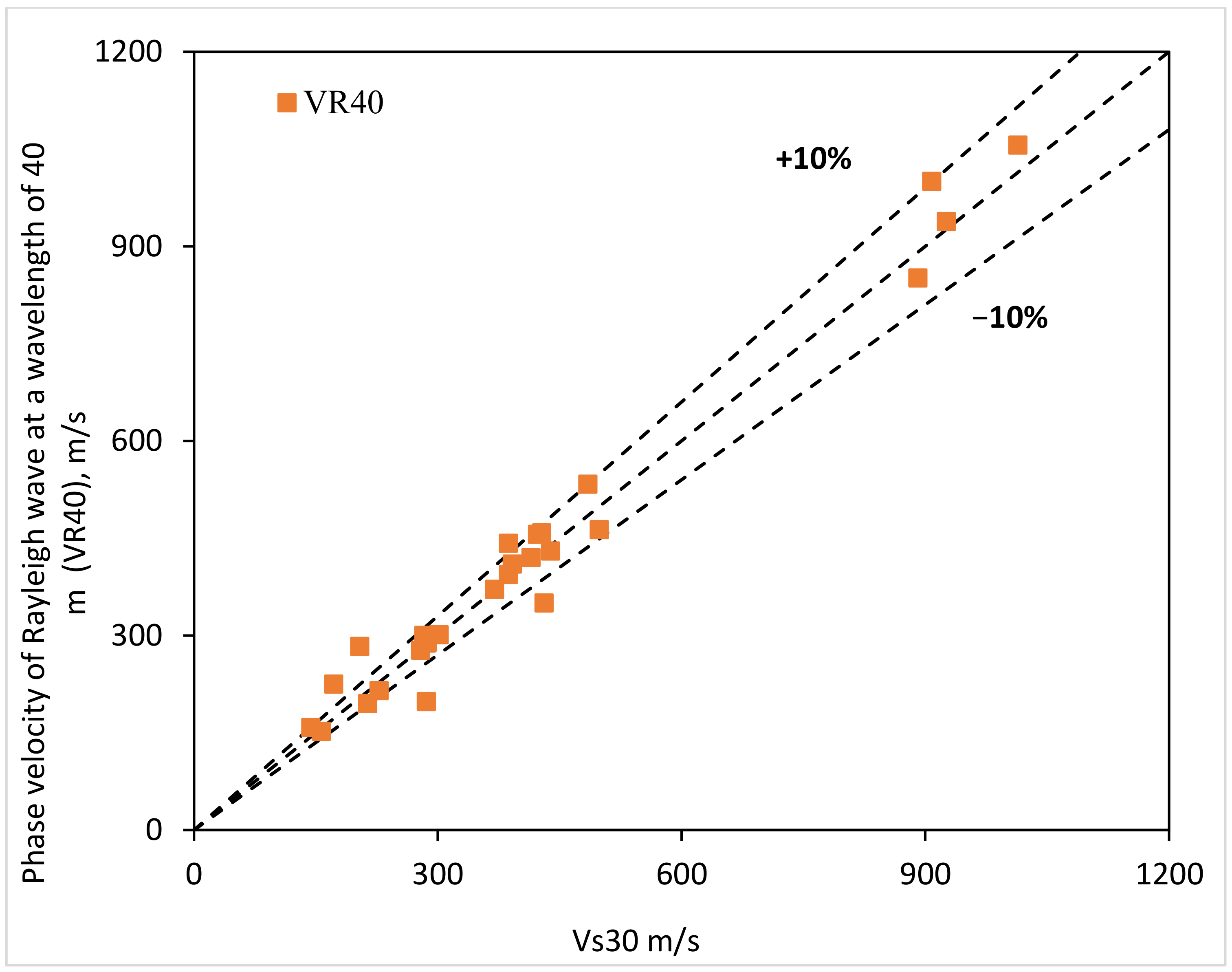
3.4. Real Data Models

Twenty-seven real data models have been collected from the survey report of the University of Puerto Rico collaborated with the US Geological Survey (Odum et al., 2007), as shown in Figure 1f. They used noninvasive seismic refraction–reflection profiling techniques to investigate near-surface shear wave velocity and compressional wave velocity. The average shear wave velocity at the top 30 meters was calculated using Equation (3) and was compared with the predictive equation results using VR36 and VR40. The results show that both VR36 and VR40 have a good relationship with Vs30, but VR40 has a better agreement with Vs30 than with VR36. This indicates that most models do not have contrast, and the results are in the acceptable zone, with some exceptional cases, as shown in Figure 8 and Figure 9. Real data models follow the two-layer synthetic approach. The results are sometimes not in the acceptable zone due to high-velocity contrast.

4. Conclusions and Suggestion

Current practices for measuring Vs30 are cost efficient and better than a single borehole, for instance, SASW, MASW, array microtremor, and refraction microtremor methods. Emphasized in this study is the potential comparison of the results from the predictive equations and formula recommendations by the international building code. In order to avoid forward modeling and inverse modeling, 53 synthetic and real data models with distinct types of vs. profiles were used, to determine the theoretical dispersion curves. VR36 and VR40 were used in the predictive equation, to estimate the Vs30. Several findings can be drawn from these results.

Based on the 53 different models, VR40 shows good agreement with shear wave velocity, i.e., Vs30.

Moving from stiff soil to hard rock, the velocity contrast increases, which affects the correlation. Vs30 determined by the predictive equations is not in the acceptable zone.

The first layer thickness has a significant influence on the correlation. The layer thickness is between 10 < H < 20 m, the thin layer is at shallow depth with lower shear waves velocity, and the results estimated by the correlation are not in the acceptable zone.

Vs30 is more sensitive to the shallow top lower Vs, while VR36 and VR40 are less sensitive to the vs. at shallow top depth. Hence, it is suggested to investigate VR instead of vs. at different wavelengths for seismic hazard zonation studies and site classification. When conducting surface wave investigations at a single location for determining VS30 for site classification, a complete surface wave dispersion curve would then be available for forward/inverse modeling if predicted VS30 is within 10% of a class boundary. A complete surface wave dispersion curve would then be available for forward/inverse modeling if predicted VS30 is within 10% of a class boundary. Developing a complete set of sounding data may be practical even if the VS30 method is used to analyze the data.

References

1. Abdelfattah, A.K.; Abdelrahman, K.; Qaysi, S.; Fnais, M.; Al-Amri, A. Earthquake recurrence characteristics for potential seismic zones in the southern red sea region and their hazard implications on jizan city. J. King Saud Univ.-Sci. 2022, 34, 101880. [Google Scholar] [CrossRef]
2. Akinci, A.; Cheloni, D.; Dindar, A.A. The 30 October 2020, M7. 0 Samos Island (Eastern Aegean Sea) Earthquake: Effects of source rupture, path and local-site conditions on the observed and simulated ground motions. Bull. Earthq. Eng. 2021, 19, 4745–4771. [Google Scholar] [CrossRef]
3. Boore, D.M.; Joyner, W.B.; Fumal, T.E. Estimation of Response Spectra and Peak Accelerations from Western North American Earthquakes: An Interim Report. 1993. Available online: http://w.daveboore.com/pubs_online/bjf93_ofr_93_509.pdf (accessed on 15 August 2022).
4. Boyle, A.; Anderson, M.R. Human Rights Approaches to Environmental Protection; Oxford University Press: Oxford, UK, 1996. [Google Scholar]
5. Anderson, M. Teacher Perceptions of Transformational Leadership Practices in Urban Charter Middle Schools. Ph.D. Thesis, Seton Hall University, South Orange, NJ, USA, 2022. [Google Scholar]
6. Chen, G.; Magistrale, H.; Rong, Y.; Cheng, J.; Binselam, S.A.; Xu, X. Seismic site condition of Mainland China from geology. Seismol. Res. Lett. 2021, 92, 998–1010. [Google Scholar] [CrossRef]
7. Wen, M.-Y.; Lee, C.-H.; Tasi, J.-C. Improving two-phase refrigerant distribution in the manifold of the refrigeration system. Appl. Therm. Eng. 2008, 28, 2126–2135. [Google Scholar] [CrossRef]
8. Code, P. Eurocode 8: Design of Structures for Earthquake Resistance-Part 1: General Rules, Seismic Actions and Rules for Buildings; European Committee for Standardization: Brussels, Belgium, 2005. [Google Scholar]
9. American Society of Civil Engineers. Seismic Evaluation and Retrofit of Existing Buildings; American Society of Civil Engineers: New York, NY, USA, 2017. [Google Scholar]
10. American Society of Civil Engineers. Seismic Analysis of Safety-Related Nuclear Structures; American Society of Civil Engineers: New York, NY, USA, 2017. [Google Scholar]
11. Zada, U.; Haleem, K.; Saqlain, M.; Abbas, A.; Khan, A.U. Reutilization of Eggshell Powder for Improvement of Expansive Clayey Soil. Iran. J. Sci. Technol. Trans. Civ. Eng. 2022, 1–8. [Google Scholar] [CrossRef]
12. Boore, D.M.; Brown, L.T. Comparing shear-wave velocity profiles from inversion of surface-wave phase velocities with downhole measurements: Systematic differences between the CXW method and downhole measurements at six USC strong-motion sites. Seismol. Res. Lett. 1998, 69, 222–229. [Google Scholar] [CrossRef]
13. Bazzurro, P.; Cornell, C.A. Nonlinear soil-site effects in probabilistic seismic-hazard analysis. Bull. Seismol. Soc. Am. 2004, 94, 2110–2123. [Google Scholar] [CrossRef]
14. Bazzurro, P.; Cornell, C.A. Ground-motion amplification in nonlinear soil sites with uncertain properties. Bull. Seismol. Soc. Am. 2004, 94, 2090–2109. [Google Scholar] [CrossRef]
15. Xia, J. Estimation of near-surface shear-wave velocities and quality factors using multichannel analysis of surface-wave methods. J. Appl. Geophys. 2014, 103, 140–151. [Google Scholar] [CrossRef]
16. Morino, M.; Kamal, A.M.; Muslim, D.; Ali, R.M.E.; Kamal, M.A.; Rahman, Z.; Kaneko, F. Seismic event of the Dauki Fault in 16th century confirmed by trench investigation at Gabrakhari Village, Haluaghat, Mymensingh, Bangladesh. J. Asian Earth Sci. 2011, 42, 492–498. [Google Scholar] [CrossRef]
17. Huang, H.W.; Zhang, B.; Wang, J.; Menq, F.-Y.; Nakshatrala, K.B.; Mo, Y.; Stokoe, K. Experimental study on wave isolation performance of periodic barriers. Soil Dyn. Earthq. Eng. 2021, 144, 106602. [Google Scholar] [CrossRef]
18. Passeri, F.; Comina, C.; Foti, S.; Socco, L.V. The Polito Surface Wave flat-file Database (PSWD): Statistical properties of test results and some inter-method comparisons. Bull. Earthq. Eng. 2021, 19, 2343–2370. [Google Scholar] [CrossRef]
19. Xu, P.; Ling, S.; Long, G.; Qiao, G.; Shen, Q.; Yao, J.; Zhang, H. ESPAC-based 2D mini-array microtremor method and its application in urban rail transit construction planning. Tunn. Undergr. Space Technol. 2021, 115, 104070. [Google Scholar] [CrossRef]
20. Saqlain, M. Computation of VS30 from model dispersion curve. In Proceedings of the 1st International Conference on Recent Advances in Civil and Earthquake Engineering (ICCEE-2021), Belgorod, Russia, 8 October 2021. [Google Scholar]
21. Graves, R.W. Modeling three-dimensional site response effects in the Marina District Basin, San Francisco, California. Bull. Seismol. Soc. Am. 1993, 83, 1042–1063. [Google Scholar] [CrossRef]
22. Iai, S.; Matsunaga, Y.; Kameoka, T. Strain space plasticity model for cyclic mobility. Soils Found. 1992, 32, 1–15. [Google Scholar] [CrossRef] [Green Version]
23. Odum, J.K.; Williams, R.A.; Stephenson, W.J.; Worley, D.M.; Von Hillebrandt-Andrade, C.; Asencio, E.; Irizarry, H.; Cameron, A. Near-Surface Shear Wave Velocity versus Depth Profiles, Vs 30, and NEHRP Classifications for 27 Sites in Puerto Rico; U. S. Geological Survey: Tallahassee, FL, USA, 2007.
24. Odum, J.K.; Stephenson, W.J.; Williams, R.A.; von Hillebrandt-Andrade, C. VS 30 and Spectral Response from Collocated Shallow, Active-, and Passive-Source VS Data at 27 Sites in Puerto Rico. Bull. Seismol. Soc. Am. 2013, 103, 2709–2728. [Google Scholar] [CrossRef]
25. Haskell, N.A. The dispersion of surface waves on multilayered media. Bull. Seismol. Soc. Am. 1953, 43, 17–34. [Google Scholar] [CrossRef]
26. Kausel, E.; Roësset, J.M. Stiffness matrices for layered soils. Bull. Seismol. Soc. Am. 1981, 71, 1743–1761. [Google Scholar] [CrossRef]
27. Olafsdottir, E.A.; Erlingsson, S.; Bessason, B. Open-Source MASW Inversion Tool Aimed at Shear Wave Velocity Profiling for Soil Site Explorations. Geosciences 2020, 10, 322. [Google Scholar] [CrossRef]
Figure 1. Shows the illustration of the different models. (a) Soft soil layer overlaying stiff soil (b) Soft layer overlaying soft rock (c) A weak, soft layer overlaying rock (d) A weak layer overlaying hard rock (e) Gradients synthetic earth profiles (f) Twenty-seven field data models.
Sustainability 14 13668 g001aSustainability 14 13668 g001b
Figure 2. Weak soil layer over stiff soil layer with variable depth of the 1st layer.
Sustainability 14 13668 g002
Figure 3. Weak soil layer on the soft rock with variable depth of 1st layer.
Sustainability 14 13668 g003
Figure 4. Weak soil layer overlaying rock.
Sustainability 14 13668 g004
Figure 5. Weak Soil Overlaying on the Hard Rock.
Sustainability 14 13668 g005
Figure 6. 2-layer Synthetic Representation Models.
Sustainability 14 13668 g006
Figure 7. Shows the result of synthetic gradient models.
Sustainability 14 13668 g007
Figure 8. Results of Real data models by using VR36.
Sustainability 14 13668 g008
Figure 9. Results of Real data models by using VR40.
Sustainability 14 13668 g009