Article

Influence of Variable Speed Limit Control on Fuel and Electric Energy Consumption, and Exhaust Gas Emissions in Mixed Traffic Flows

Faculty of Transport and Traffic Sciences, University of Zagreb, 10000 Zagreb, Croatia
*
Author to whom correspondence should be addressed.
These authors contributed equally to this work.
Sustainability 2022, 14(2), 932; https://doi.org/10.3390/su14020932
Submission received: 1 December 2021 / Revised: 5 January 2022 / Accepted: 11 January 2022 / Published: 14 January 2022
(This article belongs to the Special Issue Intelligent Mobility: Technologies, Applications and Services)

Abstract

:
Modern urban mobility needs new solutions to resolve high-complexity demands on urban traffic-control systems, including reducing congestion, fuel and energy consumption, and exhaust gas emissions. One example is urban motorways as key segments of the urban traffic network that do not achieve a satisfactory level of service to serve the increasing traffic demand. Another complex need arises by introducing the connected and autonomous vehicles (CAVs) and accompanying additional challenges that modern control systems must cope with. This study addresses the problem of decreasing the negative environmental aspects of traffic, which includes reducing congestion, fuel and energy consumption, and exhaust gas emissions. We applied a variable speed limit (VSL) based on Q-Learning that utilizes electric CAVs as speed-limit actuators in the control loop. The Q-Learning algorithm was combined with the two-step temporal difference target to increase the algorithm’s effectiveness for learning the VSL control policy for mixed traffic flows. We analyzed two different optimization criteria: total time spent on all vehicles in the traffic network and total energy consumption. Various mixed traffic flow scenarios were addressed with varying CAV penetration rates, and the obtained results were compared with a baseline no-control scenario and a rule-based VSL. The data about vehicle-emission class and the share of gasoline and diesel human-driven vehicles were taken from the actual data from the Croatian Bureau of Statistics. The obtained results show that Q-Learning-based VSL can learn the control policy and improve the macroscopic traffic parameters and total energy consumption and can reduce exhaust gas emissions for different electric CAV penetration rates. The results are most apparent in cases with low CAV penetration rates. Additionally, the results indicate that for the analyzed traffic demand, the increase in the CAV penetration rate alleviates the need to impose VSL control on an urban motorway.

1. Introduction

Urban motorways are key traffic roads in routes that provide traffic capacity for transit and local traffic. They mainly consist of many closely spaced on- and off-ramps. The problem of urban motorways is derived from the ever-increasing traffic demand that often leads to congestion and capacity drops. Such situations occur mainly near on-ramps caused by the local traffic that merges into the motorway mainstream flow during peak periods with increased traffic demand. This on-ramp traffic flow is characterized by a lower mean speed than the mainstream flow mean speed. The undoubtedly increased number of interactions between the mainstream vehicles and on-ramp vehicles influence the mainstream traffic flow and cause slowdowns. Thus, a bottleneck is created that decreases the safety and stability of the motorway traffic flow [1]. This disruption of motorway traffic flows strongly correlates to the increase in mean travel times ( M T T ) and total time spent ( T T S ) of all vehicles, which also increases the fuel consumption ( F C ), electric energy consumption ( E E C ), and exhaust gas emissions [2].
One traffic control approach that copes with the above problems is a variable speed limit (VSL) derived from intelligent transportation systems. VSL utilizes variable message signs (VMS) placed on urban motorways to apply tailor-made speed limits on urban motorways, which depend on the traffic state measurements, to cope with occurring congestion. It can reduce the chance of forming congestion and shock waves and can harmonize the speeds of upstream tree-flow and congested downstream traffic flow [3]. Various methods can be applied for adequately setting up VSL, with the machine-learning methods being in focus recently [4,5]. Reinforcement learning (RL) is a model-free control method that can be applied to VSL to compute optimal policies and apply appropriate speed limits [6,7]. RL performs an action for each state of the environment based on the previously determined values of the state–action pairs. Traffic states can be discretized by applying various methods for the spatial and temporal discretization that are determined by macroscopic traffic parameters’ measurements, including traffic density ( ρ ), speed (v), flow (q), and on-ramp queue length. The effectiveness of the learned control policy and the reward function is commonly evaluated by measuring total travel time ( T T T ), T T S , M T T , and total delay time.
The development of autonomous vehicles (AVs) and connected and autonomous vehicles (CAVs) has been rapidly growing in recent years. The introduction of AVs has been extensively tested for almost three decades in the fields of transportation, agriculture, logistics, and surveillance [8,9,10,11,12]. The introduction of those vehicles in traffic flows creates a new form of traffic flows, often referred to as mixed traffic flows that include AVs and CAVs with different penetration rates and human-driven vehicles (HDVs). The main characteristics of CAVs include the ability to receive information from various onboard sensing technologies, such as sensors, cameras, lidars, and radars. In contrast to HDVs, they have a high level of traffic law compliance, shorter headways, and the data exchange aspect that allows communication with the traffic infrastructure and other CAVs.
This study is the extension of our previous work [7], where we proposed a Q-learning (QL) VSL (QL-VSL) algorithm with the objective function to minimize T T S . For this research, we developed a centralized QL-VSL traffic-control agent that makes the decisions to post appropriate speed limits and sends the speed-limit information directly to CAVs to establish communication with roadside infrastructure. The scope of this article is restricted to mixed traffic flows that contain only HDVs and CAVs with different penetration rates. Such mixed traffic flows can be expected in the near future. Furthermore, HDVs emission classes and the gasoline and diesel engine share are set according to data collected by the Croatian Bureau of Statistics [13]. Moreover, each CAV is assumed to be an electric vehicle equipped with an onboard unit (OBU) that receives the posted speed-limit information. The QL-VSL agent sends the posted speed limit to CAVs by a roadside unit (RSU) when they enter the VSL area. Therefore, the classical VMS is redundant in mixed traffic-flow scenarios that contain CAVs. Alternatively, a virtual representation of VMS is placed to impersonate the beginning of the VSL area. For the purpose of this study, the delay of the communication network and errors in the information transmission are disregarded.
The main contribution of this study is the application and comparison of two optimization criteria of the QL-VSL control strategy to reduce traffic congestion, fuel and energy consumption, and exhaust gas emissions, utilizing CAVs as the actuators for enforcing the speed limit. The application of QL-VSL for mixed traffic flows, with realistically parametrized engine models and electric vehicle models, and analysis of two reward functions is emphasized. The ramifications of the proposed QL-VSL with two different reward function approaches are compared with baseline (no control) scenarios and rule-based VSL (RB-VSL) strategy results under various CAV penetration rate traffic-flow scenarios to analyze the effect on macroscopic traffic parameters such as T T S , M T T , speed and density, and F C , E E C , and exhaust gas emissions.
This article is organized as follows. Section 2 gives an overview of previous studies on the subject. Section 3 describes the fundamentals of VSL and an overview of QL. Section 4 provides insights into the QL-VSL application. Section 5 provides an overview of the simulation model used, and Section 6 presents the results and analysis of our experiments. In Section 7, a discussion about obtained results is given. The last section presents the conclusion and possible further work of this study.

2. Related Work

Recent studies [14,15,16,17,18] have made a more comprehensive review of VSL strategies for HDV flows. On the other hand, the ability to integrate QL-VSL in HDV flows was analyzed in [6,19,20,21,22]. In [19], the motorway traffic flow was optimized with QL applied to VSL by predicting traffic behavior. A vector with six normalized variables determined the traffic states. The proportional negative T T S was set as the optimization criteria. The oscillations of consecutive speed limits were limited not to exceed 20 km/h and were included in the reward function. In [6], the state description was done by defining features by three approaches, including the radial basis function and tile and coarse coding. The results of the QL-VSL problem were compared and analyzed on a synthetic motorway model. An RL-based approach for VSL control, which had an objective part of potential collision-risk minimization based on the vehicles’ deceleration trajectory oscillations near the congested area, was proposed in [20]. Motorway traffic mobility and safety optimization based on a multi-agent VSL control algorithm were proposed in [21]. The goal was to hold the motorway traffic density below the critical density ( ρ c ) value, which was done by cooperative distributed QL-VSL agents. The authors in [23] proposed the QL-VSL control strategy intending to reduce travel time ( T T ) at motorway bottleneck locations that outperformed the feedback-based VSL in all tested scenarios. In [22], authors analyzed the distributed spatio-temporal multi-agent VSL control approach that dynamically adjusts the VSL zones and posts speed limits. Two VSL agents were implemented to cooperatively learn to control two segments upstream of the congestion area. Each agent has its Q-Learning algorithm to learn its optimal policy, while the cooperation between VSL agents was performed using distributed W-learning. The approach outperformed the no-control and rule-based VSL in all analyzed scenarios by decreasing the T T S and increasing the average speed in the congested section and reducing traffic density in the congested section. In [24], the authors conducted the before–after analysis based on the Full Bayes (FB) approach to evaluate the safety effects of the VSL system on a real motorway model. The effectiveness of the FB approach was evaluated by comparing the predictive performance on the crash frequency of the FB approach. The VSL system has effectively reduced the total crash frequency in the VSL-controlled section. The FB before–after study showed that, after deploying the VSL system, the total crash count was reduced by 32.23% in the FB model.
In survey [5], a review of various VSL control approaches and applications in mixed traffic-flow scenarios was made. Studies [7,25,26,27] analyzed VSL performance in mixed traffic-flow scenarios containing HDVs and CAVs. A deep RL actor-critic model for differential VSL control that applies dynamic and distinct speed limits for each lane was proposed in [25]. The genetic algorithm, which includes data collection, traffic-state prediction, an optimization process, and the objective function to address the problem of numerous motorway bottlenecks in mixed traffic flows, was proposed in [26]. A Model Predictive Control (MPC)-based VSL system was analyzed in [27]. It integrates state prediction and estimation, optimization of the objective function with the rolling horizon, and speed limit action computation. The multi-criteria reward function was formulated using traffic measurements, pollutant emission, and F C measurements. In our previous study [7], we proposed a QL-VSL-based control algorithm to minimize the T T T on the congested urban motorway segment in seven mixed traffic-flow scenarios. The QL-VSL-based approach was compared and outperformed both rule-based and baseline scenarios. However, the sustainability aspect (influence on pollutant emission, EEC, and FC) of the approach was not analyzed, leaving an open question.
Studies [25,26,27,28,29,30,31] also evaluated the performance of the proposed strategies based on fuel consumption and vehicle emissions. Fuel consumption was measured in [27,29,30], while [25,26,28] measured vehicle emissions such as CO, NOx, and HC. The authors in [25] proposed the usage of the deep RL (DRL) model for a differential VSL, which stands for a VSL system that can dynamically impose a speed limit among different lanes. The model is built on the proposed actor-critic architecture based on learning discrete speed-limit changes in continuous action space. The proposed model was evaluated on the simulation with TTS, and the bottleneck speed, the number of emergency braking, and the vehicular emissions were used as training attributes. The results indicate improvements in traffic safety, efficiency, and environmental effects with reducing CO, HC, NOx, and PMx. Different effects of the compliant autonomous vehicles and the non-compliant vehicles with human drivers, in terms of submission to the implied VSL speed, are studied in [31]. The study [25] is focused on the urban areas with the intersections involved. A multi-class cell-transition model was proposed to cope with the stop-and-go vehicle’s behavior at the intersections and to reduce energy consumption. The result shows improvements in reducing energy consumption on the margin of 10 to 40%. The same model is used in [26] for CAVs in a motorway environment. The objective function was formulated to smooth the vehicle speed when transitioning between consecutive cells to harmonize the speed transition. A genetic algorithm was then adopted to solve the VSL optimization problem. Improvement in emission reduction was reported in CO 2 and NOx with up to 10%. In [27], the authors used the MPC approach for VSL to focus on individual driver behavior by measuring acceleration and deceleration. The results imply the reduction in fuel consumption up to 16% with the AVs penetration rate of 100%. The results also show that even if 100% of the penetration rate of AVs is used, multi-criteria optimization is crucial to use the full VSL benefits in the scenario with the mixed traffic flow.
In [28], the extension of VSL called C-VSL was proposed and compared to classical VSL. Infrastructure-to-vehicle (I2V) communication was utilized to set individual AV speed limits to harmonize traffic flow and reduce exhaust gas emissions. Multiple VMSs were utilized as RSUs to send each vehicle information about posted speed limits. The approach was evaluated using traffic simulation showing distinct benefits in lower acceleration rates, harmonized flow, and reduced emissions of NOx and HC. In [29], the impact of AVs on a real motorway system in various motorway traffic-demand scenarios, including free-flow traffic (≈ 0.5 · capacity), lightly congested traffic (≈ 0.7 · capacity), heavily congested traffic (> 0.95 · capacity), and future traffic (3 times greater than heavily congested traffic) conditions were analyzed. Multiple measures of effectiveness (MoEs) were collected to analyze the impact on safety, mobility, fuel consumption, and emissions such as speed, M T T , and lane occupancy. The results indicated gradual MoEs improvement with the AV penetration rate. The study reports the fuel consumption reduction by using VSL from 10 to 31% and significant emissions reduction. In [30], the authors analyzed the impact of speed control of AVs before they enter the controlled segment on an observed motorway. The Hamiltonian analysis was applied to optimal control to derive each AV’s optimal acceleration and deceleration. Fuel consumption and emissions were reduced by minimizing the accelerations or decelerations for each AV entering the controlled segment until a specified time. The results significantly improved travel time and fuel consumption by 22% and 30%, respectively. Three varying traffic demands were used to analyze the effectiveness of the proposed control method. The results were compared to the baseline scenario, the VSL algorithm (using the shock-wave theory proposed in [32]), and a modified vehicular-based speed-harmonization algorithm proposed in [33].
The “range anxiety” of electric-vehicle drivers, which refers to the driver’s fear of consuming all the available electric energy before the trip end, is one of the primary motivations for research in the field of energy consumption. Electric-energy consumption was modeled in [34] to obtain a precise range estimation. The model was validated using a commercial electric vehicle and includes a vehicle powertrain system, longitudinal vehicle dynamics, transmission, and a battery model. The model achieved an accuracy score of 2% to 6% error compared to experimental results. The driving range and electric-vehicle energy consumption were also studied in [35] by using a microscopic simulation. The authors developed a model of a pure battery-electric vehicle, which is calibrated with the experimental dataset. The validation error of the model was below 5%, and the main influence factors for the energy consumption were extracted. The main factors were the average vehicle speed, the running time, the braking frequency, and the congested traffic. The simulation of an electric vehicle on the microscopic level was also conducted in [36]. In it, the authors focused on the gap between real-world energy consumption and declared consumption values. The simplified vehicle-specific power model was presented and evaluated on standard driving cycles. The model showed improvements over other proposed models by introducing the charging power function for describing energy flow during braking. The authors in [37] studied the energy consumption and greenhouse-gas emissions of electric AVs. The case study was conducted on a mid-sized electric AV taxi dataset based on common driving cycles. The study results showed the energy consumption from 325 to 397 Wh/km, and the reported energy consumption was 6.5% larger for cars with human drivers than autonomous ones.
The use of CAVs as the mobile actuators for cooperative VSL and speed control systems was analyzed in [38,39]. The main goal was to use CAVs to adjust the speed limits on a motorway by applying the appropriate speed limits to maximize the mainstream flow and to reduce the delay time of vehicles. Therefore, our research draws the motivation to utilize CAVs as mobile speed-limit actuators to analyze the impact of applied control on the total time spent, total energy consumption, fuel consumption, and exhaust gas emissions, especially in the context of the current dawn of mixed traffic flows with an increased share of vehicles having some driving automation included as standard equipment.
In all the previous works, the impact of centralized control of CAVs in mixed traffic flows on total energy consumption, fuel consumption, and exhaust gas emissions was not analyzed. The motivation and emphasis of this study was to fill in the gap between previous studies that did not emphasize the reduction in the measures mentioned above. Finally, this study contributes to sustainable traffic control to improve the overall quality of life in urban areas.

3. Applied Methodology

This section presents the overview of VSL and QL used for this research.

3.1. Variable Speed Limit

VSL is a control approach that indirectly controls the mainstream traffic-flow speed, affecting the mainstream flow dynamics. VSL potentially eliminates the need for transport infrastructure expansion by not adding additional traffic lanes and by effectively increasing the operational capacity of the existing transport network. The performance of the traffic-control systems was assessed by measures such as T T expressed in seconds (s), T T T , and T T S determined by the travel time of all vehicles on the controlled segment of the motorway, expressed in ( v e h · h ). The flow of incoming vehicles nearing the bottleneck can be controlled and reduced by posting an appropriate speed limit [40]. By doing so, the further capacity drop is avoided, and the congestion can be relieved more quickly. VSL can also be used to achieve traffic flow that is less or equal to the maximum capacity of the bottleneck area. In addition, VSL can have a preventive effect that can delay the capacity drop caused by a sudden increase in demand on bottleneck areas. The likelihood of an incident occurring is also reduced as VSL also contributes to the harmonization of speed limits [41].
The influence of the VSL on the fundamental traffic diagram was quantitatively described in the study [42]. It implies that the critical density of traffic flow ρ c will increase with the speed-limit reduction using a fundamental diagram model. Characteristics of a stable traffic flow are shown in [43], which are described by traffic density ρ less than the critical density ρ c , where stable traffic flow represents the traffic conditions without many interactions between vehicles and traffic flows running smoothly. VSL impacts the traffic flow by reducing mean flow speed and higher density due to more harmonized traffic speeds than VSL-free traffic flow.
The impact of the VSL on the unstable traffic flow is summarized in [40]. Unstable traffic-flow conditions occur when traffic density reaches a value above the critical density ( ρ > ρ c ). As a result, interactions between vehicles become more frequent, and this kind of disruption could lead to a traffic shock wave, which can propagate in a chain reaction that can create additional traffic jams. The VSL implementation, spatially placed in front of a bottleneck area, can reduce or prevent the shock wave by speed harmonization.
Authors in [44] analyzed traffic parameters’ disruption where CAVs penetration rates were ranging from 0 to 100%. The flow–density relation and speed distributions were analyzed with two values of time headway. In the case of a time headway of 0.5 s, traffic flow was increased by 2000 veh/h. In the other example where the headway was set to 1.1 s, traffic flow was increased by up to 500 veh/h. The influence of the CAVs penetration rate resulted in reducing distributions and speed differences at high penetration rates. The authors in [45] analyzed the lane capacity for different CAV penetration rates. The lane capacity was increased by 188.2% with the incremented rates from 0 to 100%. In the other case, lane capacity was increased from 2046 to 6450 veh/h/ln when the traffic was composed of CAVs and HDVs, with the CAVs penetration rate of 100%. A similar study was conducted in [46], where the results showed the increase in the ρ c by 37% with the CAVs penetration rate of 70% and the 42% increase of the operational capacity under ρ c .

3.2. Q-Learning Algorithm

QL is an off-policy RL algorithm that learns the best action to apply at any given environment state. It is considered off-policy because the learning function learns from actions outside the current policy, like taking random actions, and therefore, a policy is not needed. The learning ability of the algorithm is based on the hypothesis that by visiting each state–action pair infinitely many times, the agent’s Q-function converges to an optimal mapping of states and actions. The agent receives feedback about the effect of the action taken through rewards or penalties, and each action performed causes a response from the environment. The main objective of the QL agent is to maximize its received reward for each state–action pair.
Problems solved using RL algorithms are commonly formulated as Markov Decision Processes (MDPs). An MDP is composed of a collection of environment states S, a collection of available actions A, a reward function R(s, a), and a transition function T(s, a, s )→[0, 1], which is a probability of moving from one state to another [47]. After the learning process has been performed, the obtained Q-function has the highest Q-value in each given state and is interpreted as the optimal state–action pair. The QL algorithm iteratively updates the stored Q-values for each state–action pair using the obtained reward from the environment [48]:
Q * ( s t , a t ) ( 1 α ) Q ( s t , a t ) + α ( r t + γ max a A Q ( s t + 1 , a ) ) ,
where Q ( s t , a t ) is the obtained Q-value for the selected state–action pair ( s t , a t ) at time step t; γ is the discount factor that determines the value of the future rewards; r t + 1 is the reward received from the environment for the chosen action a t in state s t ; s t + 1 is the new state; and α is the learning rate that determines the update rate of the Q-value in each iteration.

4. Modeling Q-Learning-Based Variable Speed Limit

Modeling of the VSL problem as an MDP can be done by assigning the QL agent to post proper speed limits [6,7,19,21,23]. The QL agent chooses and activates the calculated speed limit value for every control time step and is given the feedback (reward) to evaluate actions that altered the environment state. For each traffic-related environment state s t , the agent will execute an action a t from a set of defined actions A, which are discrete speed limits to be imposed on the motorway.
This study differs from the classical QL algorithm by implementing two look-ahead distances (states) that increase the effectiveness of the algorithm application for VSL as presented in [7,49]. This modification allows the agent to have more insight into how its actions affect future states and, thus, increases the performance of QL-VSL. This future state influence is incorporated by using two-step temporal difference λ in the QL algorithm (1) as shown below:
Q * ( s t , a t ) ( 1 α ) Q ( s t , a t ) + α ( s t , a t ) ( r t + λ r t + 1 + λ 2 max a A Q ( s t + 2 , a t + 2 ) ) ,
where λ emphasizes distant lookaheads by replacing the γ parameter in the original QL algorithm. The learning rate α is reduced gradually to deal with the non-deterministic behavior of traffic while allowing the agent to converge to near-optimal Q-values for each pair of states and actions [23]. The learning rate α is changed according to:
α ( s , a ) = 1 1 + n v ( s , a ) θ + c ,
where n v ( s , a ) represents the number of visits for each state–action pair, and θ is the constant that determines the update rate and is selected by performing a sensitivity analysis. The larger the θ value is, the more aggressive the learning is for the agent, which in turn means a lower number of iterations needed to learn the optimal policy, which may affect the quality of the learning process and calculated Q-values, and c is a constant value of 0.05 to ensure that the learning rate never reaches zero. To allow the agent to balance between exploration and exploitation, the ϵ g r e e d y policy was applied. The parameter ϵ ranges from 1 to 0 and was updated using:
ϵ = 25 10 5 · n 2 + 1 , if n < 50 e 1 n 30 + c , 0 if n 50 ,
where n represents the current simulation number. During the learning process, the ϵ parameter was gradually decreased to allow more exploitation in the later stages. The parameter ϵ was modeled to decrease the exploration phase as the Q-values for state–action pairs are updated. Before the simulations are started, all Q-values are initialized to 0. Thus, the ϵ value is very high at the beginning and is decreased by a parabolic formula from simulation 1 to 50 to maintain a higher probability of exploration. By doing so, we ensure that all the state–action pair Q-values have at least a starting value after performing random actions. After 50 simulations, ϵ was exponentially reduced until it converged to the value of c ( 0.05 ). This allowed the agent to have a slight chance of exploration in later stages of learning. The parameters of Equation (4) were obtained by performing multiple simulation scenarios with various ϵ parameter values and observing the effect on QL-VSL convergence on our simulation framework and traffic demand. Table 1 shows all the parameter combinations used in this study.

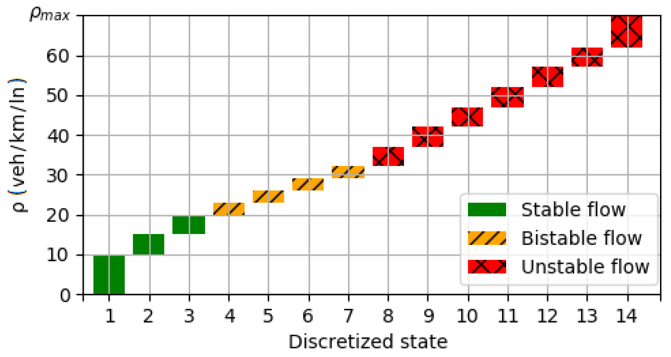
4.1. State–Action Space Description

In the case of applying QL to the traffic environment, the state–action space needs to be accurately defined. The environment in this study was the simulated urban motorway, from which we can derive macroscopic parameters from the microscopic measurements. More details are available in our previous study [7]. Traffic density ( ρ ) measured at the mainstream in the area of interest placed near the second on-ramp r 2 was defined as state representation. By discretizing the measured ρ , 14 possible states were defined, where ρ 10 veh/km/ln is state 1, to ρ > 62 veh/km/ln as state 14 (Figure 1). The increment of discretization was smaller near the ρ c , to allow VSL a more fine-tuned control to maximize the performance and try to retain traffic density near the ρ c value since traffic flow (q) has the highest theoretical value close to ρ c .
The set of available actions was defined as A = { 60 , 70 , 80 , 90 , 100 , 110 , 130 } km/h. The set of actions was additionally limited in a way that did not allow changes exceeding 30 km/h to prevent large oscillations between consecutive imposed speed limits to ensure safety and stability.

4.2. Analyzed Reward Functions

As mentioned before, the agent receives information about the environment through rewards or penalties through feedback from the environment. After each action is executed, the agent waits for the environment to respond in the form of a reward. The goal of the QL agent is to maximize its received reward for each possible pair of states and actions. We analyzed two reward functions: proportional T T S and proportional total energy consumption ( T E C ).

4.2.1. Proportional Total Time Spent Reward

The first analyzed reward was set to be as measured proportional T T S in the area of interest according to:
r T T S = 10 3 i = 1 N T T S i ,
where i is the index of the vehicle that traveled through the area of interest in the control time step, and N is the total number of vehicles that traveled through the area of interest. The reward function is proportional to the constant number 10 3 since the goal is to minimize the T T S of all vehicles that pass through the area of interest. Setting the reward this way reduces the time spent on N vehicles in the area of interest, therefore relieving the congestion as quickly as possible. For this research, we selected θ and λ values of 0.9 and 0.9, respectively, based on the extensive sensitivity analysis made. The results for each combination of those QL hyper-parameters can be found in Table A1 in Appendix A. Those selected values provided the best-combined results for all seven CAV penetration-rate scenarios.

4.2.2. Proportional Total Energy Consumption Reward

The second analyzed reward was set to be the obtained proportional T E C for the entire analyzed motorway section measured in kWh. The E E C of CAVs is measured in kWh, and F C for HDVs is measured in liters, so the reward function includes the conversion of F C [l] to kWh, and it was calculated according to:
r T E C = 10 3 i = 1 m ( k · F C i ) + j = 1 n E E C j ,
where the constant k was set to 10.38 based on the share of gasoline-propelled engines ( 0.43 ), and the share of diesel-propelled engines ( 0.57 ) multiplied with the conversion values of liters of gasoline ( 9.61 ) and diesel ( 10.96 ) to kWh, respectively, according to to [50]. The value i represents the index of a particular HDV that traveled through the motorway section, and j represents the index of electric CAV that traveled through the motorway section. The values m and n represent the total number of HDVs and electric CAVs that traveled through the motorway section, respectively. The reward function was again set to be proportional to the constant number 10 3 since the goal was to minimize the T E C of all vehicles that passed through the entire motorway section. Setting the reward this way minimizes the T E C of m and n vehicles in the analyzed motorway section, therefore reducing both F C and E E C . For this research, we selected θ and λ values of 0.8 and 0.7, respectively. The same sensitivity analysis of QL hyper-parameters can be found in Table A1 in Appendix A.

5. Simulation Setup

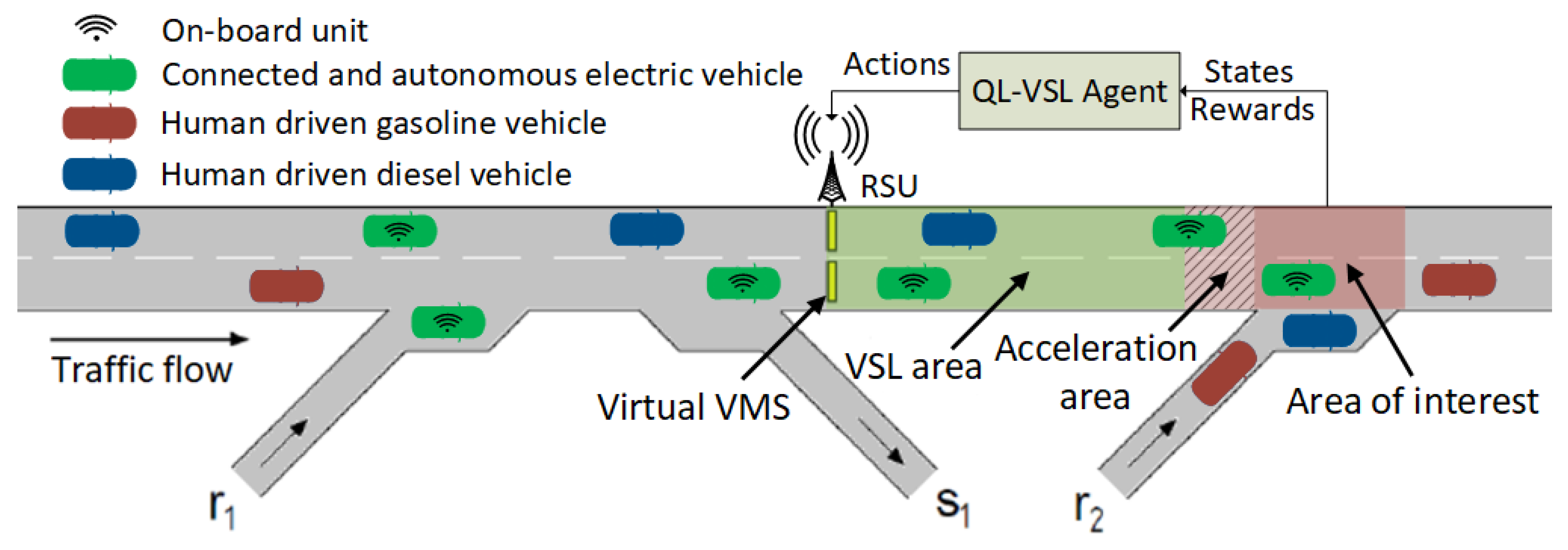
5.1. Simulation Model

The performance of the proposed QL-VSL control approach with both reward functions was verified on a synthetic motorway segment model obtained from [7] and shown in Figure 2. The constructed model was 8 km long and contained two on-ramps ( r 1 and r 2 ) and one off-ramp ( s 1 ). Note that Figure 2 is not to scale with the actual model. The functional VSL area was 500 m long, while the acceleration area was 100 m long and placed downstream and adjacent to the VSL area. The application of the acceleration area was demonstrated to be useful in [3]. Microscopic traffic-simulator simulation of urban mobility (SUMO) was used to create and perform microscopic traffic simulations [51]. The TraCI interface in SUMO was used to connect SUMO with a Python script thatallowed for the direct control of the simulation while also allowing the required traffic and ecological measurements to be recorded. Each simulation run lasted for 2 h, while the control time step was set to a 5 min interval.
The following key HDV and CAV parameters were calibrated in the SUMO simulator [52]. The driving imperfection parameter σ was set to 0.7 and 0 for HDVs and CAVs, respectively, where the value 0 denotes perfect driving. The SUMO parameter S p e e d D e v represented the speed limit deviation of vehicles and was set to 0.2 and 0.05 for HDVs and CAVs, respectively. Both vehicle classes parameter S p e e d F a c t o r was set to 1, which determines the desired driving speed multiplied by the speed limit on a given motorway segment. The parameter τ expressed in [ s ] was set to 1.1 and 0.5 for HDVs and CAVs, respectively, which represents each vehicle’s desired (minimum) time headway. The proposed QL-VSL approach was applied separately for each scenario. Therefore, its Q-function was learned independently for each scenario. The HDVs share in mixed flows were modeled in a constant ratio of 43 % of gasoline-propelled vehicles and 57 % of diesel-propelled vehicles with a Euro 4 emission norm, respectively, according to data collected by the Croatian Bureau of Statistics [13]. CAVs electric propulsion and vehicle parameters were modeled according to the available data from the mid-ranged electric vehicle from the car manufacturer Volkswagen model ID3 PRO [53]. Those parameters include the battery capacity, which was set to 77 kWh; the engine power set to 150 kW; the vehicle mass set to 1850 kg; and the air-drag coefficient set to 0.27 . The in-built SUMO emission model PHEMlight was adopted to gather the needed vehicle emissions [54,55].

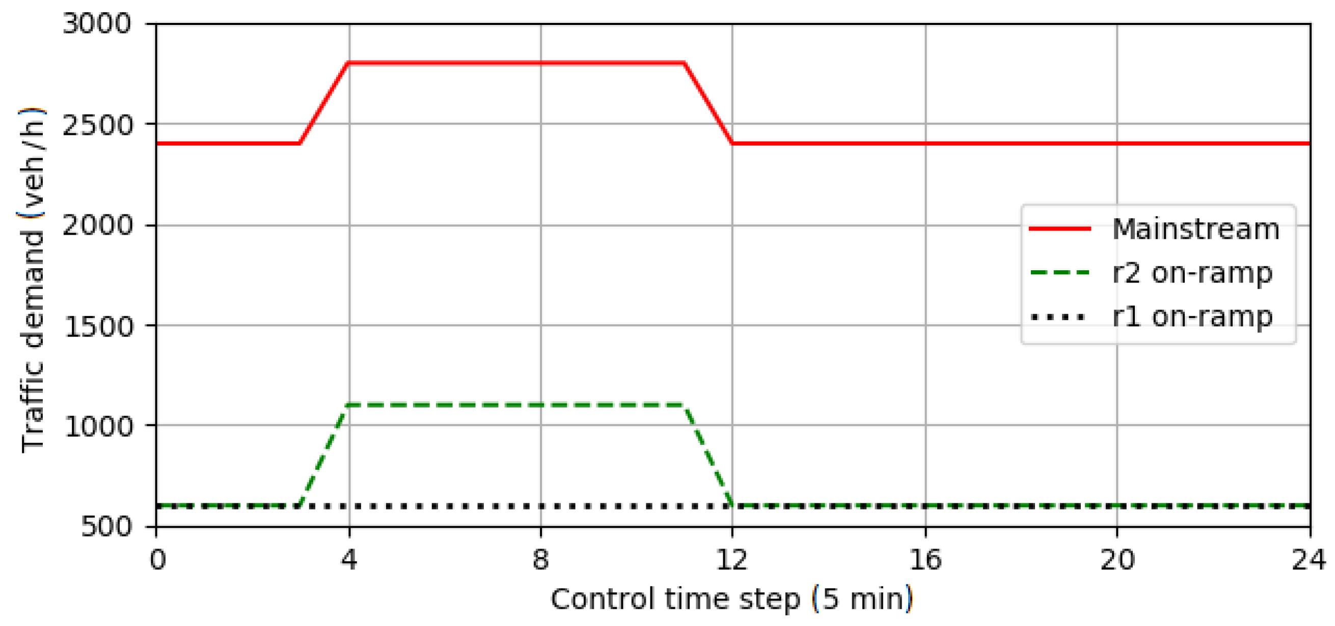
5.2. Traffic Scenarios
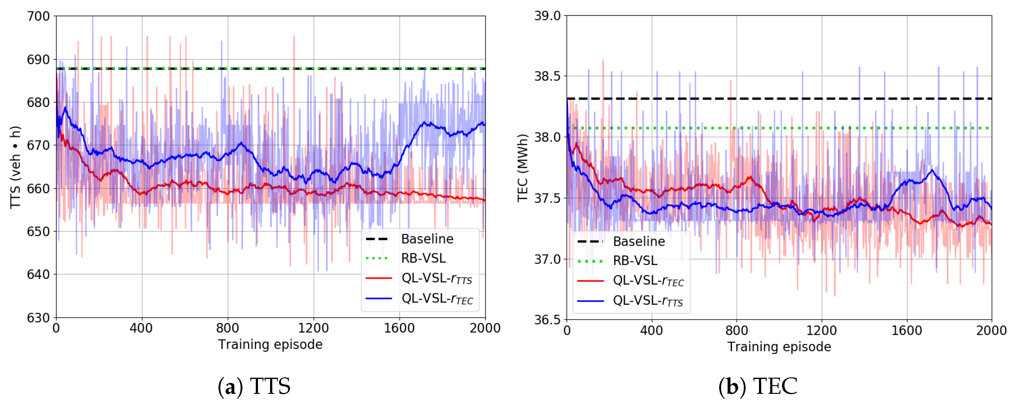
Seven simulation scenarios were formulated by increasing the CAV penetration rate from 0 to 100 % , creating various mixed traffic flows. As mentioned, the ratio of gasoline- and diesel-propelled vehicles in the decreasing share of HDVs was the same in all scenarios. Traffic demand was designed in such a way to imitate increasing traffic demand during peak hours, as shown in Figure 3.
Traffic measurements of ρ m , v m , and M T T used for state representation and controller evaluation were obtained every 5 ( s ) during the control-time step. The T T S was measured cumulatively for every simulation step ( 0.5 s) during the simulation, while for other measurements, the mean was calculated for each control time step. T T S and M T T were measured on the entire modeled motorway segment, while ρ m and v m were measured only in the area of interest shown in Figure 2. F C , E E C , CO2, CO, NOx and PMx were measured for each vehicle every simulation step. It is important to note that CO2, CO, NOx and PMx were measured only from the exhaust emissions, and other factors that potentially affect these measurements were not taken into account.

6. Results

This study compared the results to a baseline simulation without any VSL control (speed limit constant 130 km/h). Then, 2000 simulations for each defined scenario were performed to learn the QL-VSL policy. The converging trend of the QL-VSL policy was visible even after 1000 simulations. Additionally, the results were compared with the RB-VSL algorithm, which was modeled according to the highway capacity manual (HCM)-defined Levels of Service (LoS) [56] and density measurements [57]. Thus, the speed limit values were set according to [7]:
v V S L = 130 , 0 < ρ 16 110 , 16 < ρ 23 100 , 23 < ρ 26 0 90 , 26 < ρ 30 0 80 , 30 < ρ 38 0 70 , 38 < ρ 45 0 60 , ρ > 45 ,
where v V S L is the speed limit expressed in km/h, and ρ is density expressed in veh/km/ln. The set of available actions for RB-VSL in a particular control-time step was also limited not to exceed 30 km/h between two consecutive control-time steps. For each LoS, the speed limit was preset so that when the density reached the threshold for a specific LoS, a different speed limit was set for each control-time step.
For example, the best LoS A had a density threshold of 16 veh/km/ln and a speed limit of 130 km/h, while the worst LoS F had a density threshold of 45 veh/km/ln and a minor possible speed limit of 60 km/h. In all of the analyzed control strategies and baseline, a VMS was used to post speed limits in the scenario with 0% of CAVs since the traffic flow had HDVs only. The other scenarios that include CAVs in the mixed traffic flow utilized CAVs as VSL speed-limit actuators without a regular VMS to mimic future mixed traffic flows. The results summarized in Table 2 show the obtained results for the reward function being proportional T T S in the area of interest. In contrast, Table 3 shows the obtained results for the reward function being proportional T E C .
Figure 4 shows the convergence of the main objective for respective reward functions: proportional T T S (Figure 4a) and proportional T E C (Figure 4b). Both figures show the representative scenario of 30% of the CAV penetration rate, while all other scenarios behave similarly regarding the convergence of analyzed reward functions. The T T S for the QL-VSL control strategy converged to 657.8 veh·h after approximately 1500 training episodes and continued to drop slowly. On the other hand, the T E C for the QL-VSL control strategy converged to 37.3 MWh after 1600 training episodes but was still fluctuating and could be potentially reduced further after more training episodes were performed.
The results for QL-VSL with r T T S reward function shown in Table 2 indicate that both T T S and M T T decreased significantly by just introducing electric CAVs that inherently have better driving characteristics. For the low CAV-penetration-rate values, the improvements in QL-VSL were more pronounced. The results indicate that for the 0% CAV penetration rate scenario, both T T S and M T T improved by 1.55% and 2.27%, respectively. Compared to the baseline scenario, RB-VSL improved T T S and M T T by 1.36% and 2.32%, respectively. The mixed traffic-flow scenario with a low 10 % CAV penetration is highlighted since it is more probabilistic to appear in the near future. Both T T S and M T T improved in the 10 % CAV scenario by 2.13% and 0.33%, respectively, compared to baseline. The largest improvements for QL-VSL were measured for the scenario with a 30 % CAV penetration rate. QL-VSL managed to reduce T T S and M T T by 4.55% and 3.1% compared to the baseline scenario, respectively. Furthermore, mean ρ m was significantly improved by 9.89%, while F C and E E C were improved by 2.86% and 0.51%, respectively, compared to the baseline scenario. Emissions of CO 2 , CO , NO x , and PM x were reduced by 2.91%, 0.27%, 2.4%, and 2.3%, respectively.
The results for QL-VSL with the r T E C reward function shown in Table 3 also managed to improve all macroscopic traffic parameters and exhaust gas emissions, despite the focus of the reward function being T E C , F C , and E E C . For the low CAV-penetration-rate values, the improvements in QL-VSL were more pronounced. As the results indicate for the 0% CAVs, T E C and F C were improved by 2.14%, while RB-VSL improved T E C and F C by 1.21% compared to the baseline scenario. The QL-VSL for the mixed traffic-flow scenario with 10 % of CAVs improved T E C , F C , and E E C by 0.78%, 0.76%, and 1.22%, respectively, compared to baseline. The largest improvements for QL-VSL were measured for the scenario with a 30 % CAV penetration rate. QL-VSL managed to reduce T E C , F C , and E E C by 2.65%, 2.95%, and 0.04% compared to the baseline scenario, respectively. Furthermore, the mean ρ m was significantly improved by 8.44%, while T T S and M T T were improved by 4.14% and 2.47%, respectively, compared to the baseline scenario. Emissions of CO 2 , CO , NO x , and PM x were reduced by 2.83%, 0.12%, 2.58%, and 2.3%, respectively.

7. Discussion

The improvements in T T S , M T T , mean v m , and mean ρ m under different CAV-penetration-rate scenarios are shown in Figure 5. The results indicate that both T T T and M T T decreased significantly by introducing CAVs into the existing traffic flow, creating mixed traffic flows (visible in Figure 5a,b). This is due to the improved driving characteristics of CAVs compared to HDVs. The results for QL-VSL with r T T S performed better regarding the reduction in T T S for scenarios with 10%, 30%, and 50% CAV-penetration rates, while QL-VSL with r T E C performed better in the rest of the scenarios, excluding the scenario with 100% CAVs. The results for QL-VSL with r T T S performed better regarding the reduction in M T T for scenarios with 30% and 50% CAV penetration rates, while QL-VSL with r T E C performed better in the rest of the scenarios, excluding the scenario with 100% CAVs. On the other hand, RB-VSL managed to outperform QL-VSL with both reward functions in mean v m for scenario 0% CAVs and QL-VSL with r T T S reward function in scenarios with 50% and 90% CAV penetration rates (visible in Figure 5c).
The results for QL-VSL were most significant for the measured mean ρ m in the area of interest. The obtained mean ρ m results for QL-VSL with reward function r T T S for a scenario with 30% CAVs was 30.2 veh/km/ln, while the baseline measurement was 33.5 veh/km/ln, with an improvement of 9.89%. QL-VSL with the reward function r T T S managed to improve mean ρ m significantly for the scenario with 90% CAVs by 17.22% from 23.4 veh/km/ln to 19.4 veh/km/ln compared to the baseline scenario (visible in Figure 5d).
The results of QL-VSL for both reward functions regarding E E C , F C , CO 2 , CO , NO x , and PM x under different electric CAV-penetration-rate scenarios are shown in Table 2 and Table 3. The results indicate that all exhaust gas emissions inherently decreased significantly by introducing CAVs into the mixed traffic flow since they have an electric motor rather than gasoline or diesel fuel. The results for QL-VSL with r T E C performed better regarding the reduction in T E C for scenarios with 0%, 30%, 50%, and 90% CAV penetration rates, while QL-VSL with r T E C performed better in the scenario with 10% CAVs, excluding the scenarios with 70% and 100% CAV penetration rates. It is important to note that T E C decreased significantly just by introducing electric vehicles (CAVs) since they have greater energy efficiency (≈93% [58]) as opposed to gasoline and diesel HDVs (≈40–50% [59]). The result ofthe T E C measurements for the baseline no-control strategy was reduced from 50.66 MWh for the 0% to 14.63 MWh for 100% CAV-penetration-rate scenario.
The results for QL-VSL with r T E C performed better regarding the reduction in F C for scenarios with 0%, 30%, 50%, 70%, and 90% CAV penetration rates, while QL-VSL with r T E C performed better in a scenario with 10%, excluding the scenario with a 100% CAV penetration rate. On the other hand, the E E C was worsened in scenarios with 50%, 70%, and 90% CAV penetration rates for both reward functions, which means that the QL-VSL with reward function r T E C prioritized the reduction in F C rather than E E C , which correlates well with the general r T E C reward function calculation according to Equation (6). This is due to the energy value of one liter of gasoline and one liter of diesel having a high energy value. HDVs have much lower energy efficiency than electric CAVs.
The QL-VSL results for exhaust gas emissions of CO 2 , NO x , and PM x were all improved for all scenarios, excluding the scenario with a 100% CAV penetration rate. Both QL-VSL reward functions outperformed baseline scenarios and RB-VSL, with QL-VSL with reward function r T E C having slightly better performance. The exception for exhaust gas emissions can be seen for CO measurements, where QL-VSL with reward function r T E C under-performed for scenarios with 10%, 30%, 50%, 70%, and 90% CAV penetration rates compared to the RB-VSL. QL-VSL with reward function r T T S under-performed for scenarios with 30%, 50%, and 90% CAV penetration rates compared to the RB-VSL.
One key observation is that for a scenario with a 100% CAV penetration rate, all the analyzed combinations of QL hyper-parameters, reward functions, and the RB-VSL achieved the same results as the baseline scenario with no control. This indicates that the introduction of any kind of VSL control for this simulated traffic demand is obsolete.
Regarding the convergence of both reward functions, it was observed that the QL-VSL with reward function r T T S converges faster than the r T E C criteria. Furthermore, QL-VSL with reward function r T T S seems to be more stable and less fluctuating than the r T E C , which could indicate that even more training episodes are needed to stabilize and converge.

8. Conclusions

In this study, we analyzed QL-VSL with two different reward functions r T T S and r T E C impact on macroscopic traffic parameters, total energy consumption, and exhaust gas emissions for different CAV-penetration-rate traffic scenarios. We used a synthetic motorway model, calibrated engine models, and electric-vehicle models based on real-world data. Furthermore, vehicle parameters were modeled to behave realistically with adequate simulation parameters in the SUMO microscopic simulator. The obtained results indicate that the importance of separate VSL control may become obsolete under a very high CAV-penetration-rate scenario. At least for the simulated traffic demand and a general conclusion, further analysis is needed. Furthermore, the significance of any kind of VSL control approach was more influential with low CAV-penetration-rate scenarios. Both QL-VSL reward functions managed to outperform the baseline no-control scenarios and managed to improve macroscopic traffic parameters, total energy consumption, and exhaust gas emissions.
The main objective that was achieved in this study was the overall reduction in T E C , F C , and exhaust gas emissions using QL-VSL that help to move towards sustainable traffic in urban areas. Furthermore, introducing emerging technologies like connected vehicles, AVs, and CAVs that form mixed traffic flows takes momentum and drives the implementation of fully autonomous driving. In that sense, the results of this study contribute to the development of control methods that are contributing to energy efficiency and lead to more sustainable traffic for future mixed traffic flows.
One limitation of this study is, as mentioned before, that the posted speed limit information was received only by CAVs. At the same time, HDVs have to adapt the speed according to the surrounding CAVs, which may cause the degradation of traffic safety. The safety aspect will be examined in future work by determining the traffic-flow speed-harmonization level. Furthermore, multiple control-time step intervals will also be considered as they can significantly influence the QL-VSL performance and robustness. Additionally, various traffic-demand scenarios will be analyzed from the collected real-world data.

Author Contributions

The conceptualization of the study was conducted by F.V., M.M., L.T. and E.I. The funding acquisition was conducted by E.I. The writing of the original draft and preparation of the article was conducted by F.V., M.M. and L.T. All authors contributed to the writing of the article and final editing. The supervision was conducted by E.I. Visualizations were conducted by F.V. All authors have read and agreed to the published version of the manuscript.

Funding

This work was partly supported by the University of Zagreb and Faculty of Transport and Traffic Sciences under the grants “Innovative models and control strategies for sustainable mobility in smart cities” and “Optimization of the line transport timetables for the case of electric vehicles: a proof of concept,” by the Croatian Science Foundation under the project IP-2020-02-5042, and by the European Regional Development Fund under the grant KK.01.1.1.01.0009 (DATACROSS).

Institutional Review Board Statement

Not applicable.

Informed Consent Statement

Not applicable.

Acknowledgments

This research was carried out within the activities of the Centre of Research Excellence for Data Science and Cooperative Systems supported by the Ministry of Science and Education of the Republic of Croatia.

Conflicts of Interest

The authors declare no conflict of interest. The funding institutions had no role in the design of the study; in the collection, analyses, or interpretation of data; in the writing of the manuscript; or in the decision to publish the results.

Abbreviations

The following abbreviations are used in this manuscript:
AVAutonomous Vehicle
CAVConnected Autonomous Vehicle
DQLDeep Q-Learning
EECElectric Energy Consumption
FBFull Bayes
FCFuel Consumption
HDVHuman-Driven Vehicle
I2VInfrastructure-to-Vehicle
LoSLevel of Service
MDPMarkov Decision Process
MTTMean Travel Time
OBUOn-Board Unit
QLQ-Learning
QL-VSLQ-Learning Variable Speed Limit
RB-VSLRule-Based Variable Speed Limit
RLReinforcement Learning
RSURoad Side Unit
SUMOSimulation of Urban Mobility
TECTotal Energy Consumption
TTTravel Time
TTSTotal Time Spent
TTTTotal Travel Time
VMSVariable Message Sign
VSLVariable Speed Limit

Appendix A

The following Table A1 represents the results of all combinations of QL hyper-parameters θ and λ obtained for the reward functions r T T S and r T E C . The best combination of those hyper-parameters is chosen based on the sum of improvements of T T S for QL-VSL with reward function r T T S and T E C for QL-VSL with reward function r T E C compared to baseline for all CAV penetration rate scenarios.
Table A1. Sensitivity analysis of TEC reward results.
θ λ Scenario (% CAVs)rTTS
TTS (veh·h)
rTEC
TEC (MWh)
0759.549.565
10727.745.482
30678.937.742
0.750608.729.984
70560.223.145
90479.117.114
100411.614.630
077950.003
10717.345.487
30673.137.523
0.70.850606.229.977
70552.423.342
90484.917.121
100411.614.630
0771.350.170
10728.845.474
30664.237.450
0.950613.629.982
7055223.223
90487.317.108
100411.614.630
0778.149.561
10722.545.671
30682.837.301
0.750611.129.945
70559.823.133
90484.917.122
100411.614.630
0777.849.460
10714.345.691
30669.637.412
0.80.850616.629.988
70549.123.127
90484.917.132
100411.614.630
0773.949.378
10724.845.489
30675.138.031
0.950612.829.990
70559.523.122
90485.817.108
100411.614.630
0771.350.074
10723.645.479
30671.537.428
0.750613.529.985
70560.323.165
90482.917.091
100411.614.630
073749.932
10724.745.480
30671.237.677
0.90.850614.429.986
70571.523.401
90480.417.085
100411.614.630
0770.650.660
10709.745.494
30656.537.777
0.950611.829.988
70560.923.119
90487.517.104
100411.614.630

References

  1. Grumert, E.; Tapani, A.; Ma, X. Characteristics of variable speed limit systems. Eur. Transp. Res. Rev. 2018, 10, 21. [Google Scholar] [CrossRef]
  2. Greenwood, I.D.; Dunn, R.C.; Raine, R.R. Estimating the Effects of Traffic Congestion on Fuel Consumption and Vehicle Emissions Based on Acceleration Noise. J. Transp. Eng. 2007, 133, 96–104. [Google Scholar] [CrossRef]
  3. Müller, E.; Carlson, R.; Kraus, W.; Papageorgiou, M. Microsimulation analysis of practical aspects of traffic control with variable speed limits. IEEE Trans. Intell. Transp. Syst. 2015, 16, 512–523. [Google Scholar] [CrossRef]
  4. Kušić, K.; Ivanjko, E.; Gregurić, M.; Miletić, M. An Overview of Reinforcement Learning Methods for Variable Speed Limit Control. Appl. Sci. 2020, 10, 4917. [Google Scholar] [CrossRef]
  5. Vrbanić, F.; Ivanjko, E.; Kušić, K.; Čakija, D. Variable Speed Limit and Ramp Metering for Mixed Traffic Flows: A Review and Open Questions. Appl. Sci. 2021, 11, 2574. [Google Scholar] [CrossRef]
  6. Kušić, K.; Ivanjko, E.; Gregurić, M. A Comparison of Different State Representations for Reinforcement Learning Based Variable Speed Limit Control. In Proceedings of the MED 2018–26th Mediterranean Conference on Control and Automation, Zadar, Croatia, 19–22 June 2018; pp. 266–271. [Google Scholar] [CrossRef]
  7. Vrbanić, F.; Ivanjko, E.; Mandžuka, S.; Miletić, M. Reinforcement Learning Based Variable Speed Limit Control for Mixed Traffic Flows. In Proceedings of the 2021 29th Mediterranean Conference on Control and Automation (MED), Puglia, Italy, 22–25 June 2021; pp. 560–565. [Google Scholar] [CrossRef]
  8. Van Brummelen, J.; O’Brien, M.; Gruyer, D.; Najjaran, H. Autonomous vehicle perception: The technology of today and tomorrow. Transp. Res. Part C Emerg. Technol. 2018, 89, 384–406. [Google Scholar] [CrossRef]
  9. Yu, J.J.Q.; Lam, A.Y.S.; Lu, Z. Double Auction-Based Pricing Mechanism for Autonomous Vehicle Public Transportation System. IEEE Trans. Intell. Veh. 2018, 3, 151–162. [Google Scholar] [CrossRef]
  10. Li, M.; Imou, K.; Wakabayashi, K.; Yokoyama, S. Review of research on agricultural vehicle autonomous guidance. Int. J. Agric. Biol. Eng. 2008, 2, 1–16. [Google Scholar] [CrossRef]
  11. Yu, J.J.Q.; Lam, A.Y.S. Autonomous Vehicle Logistic System: Joint Routing and Charging Strategy. IEEE Trans. Intell. Transp. Syst. 2018, 19, 2175–2187. [Google Scholar] [CrossRef]
  12. Ayub, M.F.; Ghawash, F.; Shabbir, M.A.; Kamran, M.; Butt, F.A. Next Generation Security And Surveillance System Using Autonomous Vehicles. In Proceedings of the 2018 Ubiquitous Positioning, Indoor Navigation and Location-Based Services (UPINLBS), Wuhan, China, 22–23 March 2018; pp. 1–5. [Google Scholar] [CrossRef]
  13. Croatian Bureau of Statistics. Transport and Communications-Registered Road Vehicles by Types, Age, Size of Engine and Type of Motor Energy. 2021. Available online: https://www.dzs.hr/Hrv/publication/FirstRelease/results.asp?pString=Transport%20i%20komunikacije&pSearchString=%Transport%20i%20komunikacije% (accessed on 15 October 2021).
  14. Khondaker, B.; Kattan, L. Variable speed limit: An overview. Transp. Lett. Int. J. Transp. Res. 2015, 7, 264–278. [Google Scholar] [CrossRef]
  15. Lu, X.Y.; Shladover, S. Review of Variable Speed Limits and Advisories. Transp. Res. Rec. J. Transp. Res. Board 2014, 2423, 15–23. [Google Scholar] [CrossRef]
  16. Gregurić, M.; Ivanjko, E.; Korent, N.; Kušić, K. Short Review of Approaches for Variable Speed Limit Control. In Proceedings of the International Scientific Conference on Science and Transport Development (ZIRP 2016), Zagreb, Croatia, 4 April 2016; pp. 41–52. [Google Scholar]
  17. Abdel-Aty, M.; Yu, R. State-of-practice of variable speed limit systems. In Proceedings of the 20th ITS World Congress, Tokyo, Japan, 14–18 October 2013. [Google Scholar]
  18. Tafti, M. An investigation on the approaches and methods used for variable speed limit control. In Proceedings of the 15th World Congress on Intelligent Transport Systems and ITS America’s 2008 Annual Meeting, New York, NY, USA, 16–20 November 2008; pp. 901–912. [Google Scholar]
  19. Walraven, E.; Spaan, M.T.; Bakker, B. Traffic flow optimization: A reinforcement learning approach. Eng. Appl. Artif. Intell. 2016, 52, 203–212. [Google Scholar] [CrossRef]
  20. Li, Z.; Xu, C.; Pu, Z.; Guo, Y.; Liu, P. Reinforcement Learning-Based Variable Speed Limits Control to Reduce Crash Risks near Traffic Oscillations on Freeways. IEEE Intell. Transp. Syst. Mag. 2020, 13, 64–70. [Google Scholar] [CrossRef]
  21. Wang, C.; Zhang, J.; Xu, L.; Li, L.; Ran, B. A New Solution for Freeway Congestion: Cooperative Speed Limit Control Using Distributed Reinforcement Learning. IEEE Access 2019, 7, 41947–41957. [Google Scholar] [CrossRef]
  22. Kušić, K.; Ivanjko, E.; Vrbanić, F.; Gregurić, M.; Dusparic, I. Dynamic Variable Speed Limit Zones Allocation Using Distributed Multi-Agent Reinforcement Learning. In Proceedings of the 2021 IEEE International Intelligent Transportation Systems Conference (ITSC), Indianapolis, IN, USA, 19–22 September 2021; pp. 3238–3245. [Google Scholar] [CrossRef]
  23. Li, Z.; Liu, P.; Xu, C.; Duan, H.; Wang, W. Reinforcement Learning-Based Variable Speed Limit Control Strategy to Reduce Traffic Congestion at Freeway Recurrent Bottlenecks. IEEE Trans. Intell. Transp. Syst. 2017, 18, 3204–3217. [Google Scholar] [CrossRef]
  24. Pu, Z.; Li, Z.; Jiang, Y.; Wang, Y. Full Bayesian Before-After Analysis of Safety Effects of Variable Speed Limit System. IEEE Trans. Intell. Transp. Syst. 2021, 22, 964–976. [Google Scholar] [CrossRef]
  25. Wu, Y.; Tan, H.; Qin, L.; Ran, B. Differential variable speed limits control for freeway recurrent bottlenecks via deep actor-critic algorithm. Transp. Res. Part C Emerg. Technol. 2020, 117, 102649. [Google Scholar] [CrossRef]
  26. Yu, M.; Fan, W. Optimal variable speed limit control in connected autonomous vehicle environment for relieving freeway congestion. J. Transp. Eng. Part A Syst. 2019, 145, 04019007. [Google Scholar] [CrossRef]
  27. Khondaker, B.; Kattan, L. Variable speed limit: A microscopic analysis in a connected vehicle environment. Transp. Res. Part C Emerg. Technol. 2015, 58, 146–159. [Google Scholar] [CrossRef] [Green Version]
  28. Grumert, E.; Ma, X.; Tapani, A. Analysis of a cooperative variable speed limit system using microscopic traffic simulation. Transp. Res. Part C Emerg. Technol. 2015, 52, 173–186. [Google Scholar] [CrossRef]
  29. Li, D.; Wagner, P. Impacts of gradual automated vehicle penetration on motorway operation: A comprehensive evaluation. Eur. Transp. Res. Rev. 2019, 11, 36. [Google Scholar] [CrossRef]
  30. Malikopoulos, A.; Hong, S.; Park, B.; Lee, J.; Ryu, S. Optimal Control for Speed Harmonization of Automated Vehicles. IEEE Trans. Intell. Transp. Syst. 2019, 20, 2405–2417. [Google Scholar] [CrossRef] [Green Version]
  31. Rongsheng, C.; Zhang, T.; Levin, M.W. Effects of Variable Speed Limit on Energy Consumption with Autonomous Vehicles on Urban Roads Using Modified Cell-Transmission Model. J. Transp. Eng. Part A Syst. 2020, 146, 04020049. [Google Scholar] [CrossRef]
  32. Hegyi, A.; Hoogendoorn, S.; Schreuder, M.; Stoelhorst, H.; Viti, F. Specialist: A dynamic speed limit control algorithm based on shock wave theory. In Proceedings of the 11th International IEEE Conference on Intelligent Transportation Systems (ITSC), Beijing, China, 12–15 October 2008; pp. 827–832. [Google Scholar] [CrossRef]
  33. Ma, J.; Li, X.; Zhou, F.; Hu, J.; Park, B. Parsimonious shooting heuristic for trajectory design of connected automated traffic part II: Computational issues and optimization. Transp. Res. Part B Methodol. 2017, 95, 421–441. [Google Scholar] [CrossRef] [Green Version]
  34. Miri, I.; Fotouhi, A.; Ewin, N. Electric vehicle energy consumption modelling and estimation—A case study. Int. J. Energy Res. 2021, 45, 501–520. [Google Scholar] [CrossRef]
  35. Xie, Y.; Li, Y.; Zhao, Z.; Dong, H.; Wang, S.; Liu, J.; Guan, J.; Duan, X. Microsimulation of electric vehicle energy consumption and driving range. Appl. Energy 2020, 267, 115081. [Google Scholar] [CrossRef]
  36. Luin, B.; Petelin, S.; Al-Mansour, F. Microsimulation of electric vehicle energy consumption. Energy 2019, 174, 24–32. [Google Scholar] [CrossRef]
  37. Zhang, C.; Yang, F.; Ke, X.; Liu, Z.; Yuan, C. Predictive modeling of energy consumption and greenhouse gas emissions from autonomous electric vehicle operations. Appl. Energy 2019, 254, 113597. [Google Scholar] [CrossRef]
  38. Müller, E.; Carlson, R.; Kraus, W. Cooperative Mainstream Traffic Flow Control on Freeways. IFAC-PapersOnLine 2016, 49, 89–94. [Google Scholar] [CrossRef]
  39. Vinitsky, E.; Parvate, K.; Kreidieh, A.; Wu, C.; Bayen, A. Lagrangian Control through Deep-RL: Applications to Bottleneck Decongestion. In Proceedings of the 21st International Conference on Intelligent Transportation Systems (ITSC), Maui, HI, USA, 4–7 November 2018; pp. 759–765. [Google Scholar] [CrossRef]
  40. Papageorgiou, M.; Kosmatopoulos, E.; Papamichail, I. Effects of Variable Speed Limits on Motorway Traffic Flow. Transp. Res. Rec. J. Transp. Res. Board 2008, 2047, 37–48. [Google Scholar] [CrossRef]
  41. Lee, C.; Hellinga, B.; Saccomanno, F. Evaluation of variable speed limits to improve traffic safety. Transp. Res. Part C Emerg. Technol. 2006, 14, 213–228. [Google Scholar] [CrossRef]
  42. Cremer, M. Der Verkehrsfluss auf Schnellstrassen: Modelle, Überwachung, Regelung; Springer: Berlin/Heidelberg, Germany, 1979. [Google Scholar]
  43. Carlson, R.C.; Papamichail, I.; Papageorgiou, M.; Messmer, A. Optimal Motorway Traffic Flow Control Involving Variable Speed Limits and Ramp Metering. Transp. Sci. 2010, 44, 238–253. [Google Scholar] [CrossRef]
  44. Ye, L.; Yamamoto, T. Evaluating the impact of connected and autonomous vehicles on traffic safety. Phys. A Stat. Mech. Its Appl. 2019, 526, 121009. [Google Scholar] [CrossRef]
  45. Olia, A.; Razavi, S.; Abdulhai, B.; Abdelgawad, H. Traffic capacity implications of automated vehicles mixed with regular vehicles. J. Intell. Transp. Syst. Technol. Plan. Oper. 2018, 22, 244–262. [Google Scholar] [CrossRef]
  46. Wang, Q.; Li, B.; Li, Z.; Li, L. Effect of connected automated driving on traffic capacity. In Proceedings of the 2017 Chinese Automation Congress (CAC), Jinan, China, 20–22 October 2017; pp. 633–637. [Google Scholar]
  47. Bellman, R. A Markovian Decision Process. J. Math. Mech. 1957, 6, 679–684. [Google Scholar] [CrossRef]
  48. Watkins, C.J.C.H.; Dayan, P. Q-learning. Mach. Learn. 1992, 8, 279–292. [Google Scholar] [CrossRef]
  49. Sutton, R.; Barto, A. Reinforcement Learning: An Introduction; MIT Press: Cambridge, MA, USA, 1998. [Google Scholar]
  50. Universities and Colleges Climate Commitment for Scotland. UCCCfS Unit Converter. 2010. Available online: http://www.eauc.org.uk/file_uploads/ucccfs_unit_converter_v1_3_1.xlsx (accessed on 5 October 2021).
  51. Behrisch, M.; Bieker-Walz, L.; Erdmann, J.; Krajzewicz, D. SUMO—Simulation of Urban MObility: An Overview. In Proceedings of the Third International Conference on Advances in System Simulation, SIMUL 2011, Barcelona, Spain, 23–28 October 2011. [Google Scholar]
  52. Li, D.; Wagner, P. A novel approach for mixed manual/connected automated freeway traffic management. Sensors 2020, 20, 1757. [Google Scholar] [CrossRef] [PubMed] [Green Version]
  53. Volkswagen of America, Inc. Newspress Limited. World Premiere of the Fully Electric ID.3. 2019. Available online: https://media.vw.com/en-us/releases/1198 (accessed on 28 September 2021).
  54. Hausberger, S.; Krajzewicz, D. Extended Simulation Tool PHEM Coupled to SUMO with User Guide. 2014. Available online: https://web.archive.org/web/20190527152150/https://elib.dlr.de/98047/1/COLOMBO_D4.2_ExtendedPHEMSUMO_v1.7.pdf (accessed on 28 September 2021).
  55. Institute for Internal Combustion Engines and Thermodynamics. Passenger Car and Heavy Duty Emission Model. 2016. Available online: https://www.ivt.tugraz.at/assets/files/areas/em/PHEM_en.pdf (accessed on 28 September 2021).
  56. Elefteriadou, L.A. (Ed.) Highway Capacity Manual 6th Edition: A Guide for Multimodal Mobility Analysis; Transportation Research Board, The National Academies Press: Washington, DC, USA, 2016. [Google Scholar] [CrossRef]
  57. Tišljarić, L.; Carić, T.; Abramović, B.; Fratrović, T. Traffic State Estimation and Classification on Citywide Scale Using Speed Transition Matrices. Sustainability 2020, 12, 7278. [Google Scholar] [CrossRef]
  58. Hofman, T.; Dai, C. Energy efficiency analysis and comparison of transmission technologies for an electric vehicle. In Proceedings of the 2010 IEEE Vehicle Power and Propulsion Conference, Lille, France, 1–3 September 2010; pp. 1–6. [Google Scholar] [CrossRef]
  59. Nylund, N.O. Vehicle Energy Efficiencies. In Proceedings of the IEA EGRD Workshop Mobility: Technology Priorities and Strategic Urban Planning, Espoo, Finland, 22–23 May 2013. [Google Scholar]
Figure 1. Discretized state representation [7].
Sustainability 14 00932 g001
Figure 2. Simulation model and framework [7].
Sustainability 14 00932 g002
Figure 3. Traffic demand on the mainstream and on-ramps during simulation [7].
Sustainability 14 00932 g003
Figure 4. The convergence of TTS and TEC during simulations.
Sustainability 14 00932 g004
Figure 5. Comparison of QL-VSL reward functions r T T S and r T E C impact on macroscopic traffic parameters.
Sustainability 14 00932 g005
Table 1. Combination of tested QL values.
λ 0.70.80.9
θ 0.7 0.8 0.9 0.7 0.8 0.9 0.7 0.8 0.9
Table 2. TTS reward results.
Scenario
(% CAVs)
Control
Strategy
TTS
(veh·h)
MTT
(s)
Mean vm
(km/h)
Mean ρm
(veh/km/ln)
TEC
(MWh)
EEC
(MWh)
FC
(l)
CO2
(kg)
CO
(kg)
NOx
(kg)
PMx
(kg)
Baseline790.4368.759.338.650.64-4879.011,973.0139.835.320.96
0RB-VSL779.7360.960.837.750.03-4819.911,828.9139.435.130.95
QL-VSL778.2360.459.738.149.86-4803.011,786.1138.734.930.95
Baseline725.2344.065.635.246.031.354304.710,551.5130.831.820.86
10RB-VSL718.6343.664.536.145.711.344274.710,478.8130.731.690.85
QL-VSL709.7342.966.134.345.471.344252.010,422.1130.431.570.85
Baseline687.8327.472.133.538.324.043301.98087.0105.824.800.67
30RB-VSL687.8327.172.133.538.074.023281.28035.3104.524.490.66
QL-VSL656.5317.375.930.237.314.023207.47851.3105.524.210.65
Baseline618.2302.486.125.730.016.762239.85478.676.217.070.46
50RB-VSL613.9299.786.625.430.076.762246.05490.277.717.080.46
QL-VSL611.8299.486.225.330.006.782237.25468.677.516.980.46
Baseline574.0276.095.023.423.369.671319.73224.146.710.090.27
70RB-VSL571.9273.594.923.623.359.751310.63200.847.110.000.27
QL-VSL560.9271.096.622.123.139.711292.73157.545.99.870.26
Baseline489.0235.7108.918.217.1712.89412.41006.814.93.140.08
90RB-VSL491.2236.6109.717.917.1312.87410.81001.915.13.090.08
QL-VSL487.5235.2109.517.817.1612.93407.8993.915.33.060.08
Baseline411.6206.3121.212.614.6314.63-----
100RB-VSL411.6206.3121.212.614.6314.63-----
QL-VSL411.6206.3121.212.614.6314.63-----
Table 3. TEC reward results.
Scenario
(% CAVs)
Control
Strategy
TTS
(veh·h)
MTT
(s)
Mean vm
(km/h)
Mean ρm
(veh/km/ln)
TEC
(MWh)
EEC
(MWh)
FC
(l)
CO2
(kg)
CO
(kg)
NOx
(kg)
PMx
(kg)
Baseline790.4368.759.338.650.64-4879.011,973.0139.835.320.96
0RB-VSL779.7360.960.837.750.03-4819.911,828.9139.435.130.95
QL-VSL766.8356.460.937.049.56-4774.711,717.2138.934.900.94
Baseline725.2344.065.635.246.031.354304.710,551.5130.831.820.86
10RB-VSL718.6343.664.536.145.711.344274.710,478.8130.731.690.85
QL-VSL714.0341.765.235.145.671.334271.810,468.4131.631.710.85
Baseline687.8327.472.133.538.324.043301.98087.0105.824.800.67
30RB-VSL687.8327.172.133.538.074.023281.28035.3104.524.490.66
QL-VSL659.3319.375.430.737.304.043204.47858.2105.724.160.65
Baseline618.2302.486.125.730.016.762239.85478.676.217.070.46
50RB-VSL613.9299.786.625.430.076.762246.05490.277.717.080.46
QL-VSL613.1299.686.725.229.946.782232.15458.176.116.990.46
Baseline574.0276.095.023.423.369.671319.73224.146.710.090.27
70RB-VSL571.9273.594.923.623.359.751310.63200.847.110.000.27
QL-VSL551.5266.9101.419.423.139.751289.03146.746.89.870.26
Baseline489.0235.7108.918.217.1712.89412.41006.814.93.140.08
90RB-VSL491.2236.6109.717.917.1312.87410.81001.915.13.090.08
QL-VSL481.6233.1110.817.117.1212.93403.4983.214.83.020.08
Baseline411.6206.3121.212.614.6314.63-----
100RB-VSL411.6206.3121.212.614.6314.63-----
QL-VSL411.6206.3121.212.614.6314.63-----
Publisher’s Note: MDPI stays neutral with regard to jurisdictional claims in published maps and institutional affiliations.

