Hybrid Finite-Discrete Element Modelling of Various Rock Fracture Modes during Three Conventional Bending Tests

Abstract

The numerical techniques for modelling the rock fracture have been briefly reviewed. A hybrid finite-discrete element method (HFDEM) is proposed to simulate various fracture types of rock. A fracture model is implemented in the HFDEM for simulation of the three main fracture types. In addition, the influence of the strain rate is considered during the HFDEM modelling rock behavior. Then, two typical rock mechanism tests are employed to calibrate the HFDEM. The proposed method has well modelled the rock fracture processes and can obtain reasonable stress distribution and force–displacement curves. After that, the HFDEM is used to model three convention bending tests. The obtained rock fracture processes indicates that the HFDEM can simulate various fracture types. The obtained rock strengths and fracture toughness indicate that the HFDEM can reflect the influence of the strain rate. It is concluded that the HFDEM can model the entire and complete rock fracture process during the three convention bending tests, and it also can capture the rock’s behavior on the strain rate.

1. Introduction

Rock fracture behavior has been widely studied, especially under a variety of loading conditions. The numerical method is now a popular technique for studying rock behaviors. In numerical method, the rock materials can be considered as continuum, such as finite element method, while it can also be regarded as a discontinuum, such as the discrete element method. For the continuum method, the model is treated as continuous body, and it is discretized into elements. The continuous-based method has been successfully applied in rock fracture modelling, in which the discontinuity of the rock mass can be ignored due to that the modelled scale is much larger than the existing or produced cracks in the rock mass. However, when the discontinuity of the geo-materials cannot be neglected due to the original existing original produced fractures are comparable to the interest area, the discontinuity should be taken into account.

Discontinuum-based methods are also popular tools employed in the study of rock mechanics. In the discontinuum-based methods, the rock mass is assumed to be an assembly of discrete elements [1]. Thus, the discontinuity of the rock mass has been fully considered. Since Cundall [2] proposed the distinct element method (DEM) and implemented it widely into the investigate rock fracture and resultant fragmentation process [3], discontinuum-based methods have been extensively used in various rock failure problems [4,5]. For example, the Gutiérrez-Ch et al. (2018 and 2021) used the DEM models to successfully simulate the rock response during direct shear tests and all stages of rock creep behaviour in the laboratory tests [6,7]. The representative discontinuum-based methods are the distinct element method, the bounded particle method (BPM), and the discontinuous deformation analysis (DDA) [8,9]. Compared with the continuum method, the distinct element method allows the displacement and rotation of discrete bodies. The UDEC and 3DEC might be the most common used DEM code [10] for modelling the rock fracture and result fragmentation process. The domain is divided into rigid discrete bodies in the UDEC or 3DEC, which can move, rotate, or slip during the contact interaction of the discrete bodies [10]. The fractures in DEM are modelled along the boundary of discrete bodies when the stress reaches its maximum. The bounded particle method (BPM) is a particle-based discontinuum method. The domain in this method is divides into circular and spherical rigid elements [11]. Shi and Godman (1985) proposed discontinuous deformation analysis (DDA), which is an implicit formulation of DEM [12]. The DDA employs sub-block techniques to modelling the continuous–discontinuous transition [13]. Thus, the fracture and fragmentation of rocks can be modelled along the block boundaries.

To realistically model the rock fracture process, numerical methods should be able to model the fracture initiation and propagation [14]. For this purpose, the continuum–discontinuum methods are proposed [9,15]. It should be noted that the combined or hybrid continuum–discontinuum methods are different from the coupled combined or hybrid continuum–discontinuum methods. The former can freely model the continuum and discontinuum behaviours of rocks and their transitions, while the latter adopts a physical boundary to couple the two methods.

The ELFEN might be the most widely used commercial software of the combined FEM/DEM. The Y-code is open source for the implementation of the combined FEM/DEM, originally developed by Munjiza [15]. Then, the Y-Geo was developed for the convenient use of the Y-code. The Y-code has its difficulties in modelling mixed mode fractures and lacks consideration of the loading rate and material heterogeneity [16]. To address these limitations, many extensions of the Y-code have been developed. An et al. (2017) developed Y2D/3D IDE to model the blast-induced frock fracture and resultant fragmentation processes [16]. The open source Y-code accelerates the development of the combined/hybrid FEM/DEM method, and many extensions of the Y-code have been well implemented in rock fracture and fragmentation modelling [17].

In this study, the authors developed the HFDEM, which is proposed to simulate the various rock fracture types. The fracture model and the curve are specially implemented in the HFDEM for modelling the complete rock fracture process and taking the influence of the loading rate into account, respectively. The HFDEM is verified by the simulation of typical rock mechanism test. Then, the HFDEM is used to simulate three convention point bending tests to obtain various fracture modes.

2. HFDEM for Modelling Dynamic Rock Fracture

To completely model the rock fracture process, the HFDEM needs to be able to model the rock initiation, propagation, and interaction of fractured rock and resultant fragmentation. In addition, the influence due to different loading rates should also be taken into account. Thus, in this section, the above two key components are explained in detail.

2.1. Transition from Continuum to Discontinuum

In HFDEM, the transition from continuum to discontinuum is modelled through the fracture of the discrete bodies. As illustrated in Figure 1, the stress–strain curve is divided into two parts, the stress hardening and stress softening parts, separated by the peak stress. Constitutive law is employed to model the stress hardening parts, while the opening or sliding displacement of the finite elements can describe the stress softening part.

Figure 2 illustrates the HFDEM models, which are comprised of three-node finite elements describing the deformability of the rock material and four-node crack elements describing the fracture propagation. In addition, the four-node crack elements can be distorted in the normal direction, causing tensile failure (mode-I fracture), and the tangential direction, causing shear failure (mode-II fracture). Figure 2b–d demonstrate the model under tension, shear, and combined tension and shear condition, respectively, while the corresponding stress opening/sliding curves are illustrated in Figure 3.

In HFDEM, the fractures occur at finite element edges, and the separation of the finite elements induce a bonding stress. The value of the bonding stress is related to the distortion of the four-node elements. Equation (1) illustrates the four-node elements distortion:

$$\delta ={\delta }_n\mathit{n}+{\delta }_s\mathit{t}$$

(1)

where $\mathit{n}$ indicates the unit vector’s normal direction, while $\mathit{t}$ is that in the tangential direction. ${\delta }_n$ and ${\delta }_s$ are the magnitudes of the the components of $\delta$ in the two directions.

Figure 3a indicates the stress-opening relationship for pure mode I fracture, i.e., tensile failure. It should be noted that the opening or sliding of finite elements from the element edges means the distortion of the four nodes crack elements in normal or tangential directions in the following text. As illustrated in Figure 3a, as ${\delta }_n$ increases in the normal direction, the stress increases. Before the opening reaches ${\delta }_{np}$, i.e., $0\le {\delta }_n<{\delta }_{np}$, the stress is increasing but no crack occurs. When the opening reaches a critical value ${\delta }_{np}$, i.e., ${\delta }_n={\delta }_{np}$, the stress reaches the tensile strength ${\sigma }_t$ and crack occurs. With the separation of the finite element edges continues, the opening is ${\delta }_{nu}$, i.e., ${\delta }_n>{\delta }_{nu}$, the finite elements are completely separated from the element edges, i.e., and the four-node crack element among the finite elements is removed. Thus, the tensile fracture has completed.

During the tensile rock fracture process, the normal direction bonding stress can be calculated using Equation (2):

$${\sigma }_n=\{\begin{array}{ccc}\left[2·\frac{{\delta }_n}{{\delta }_{np}}-{\left(\frac{{\delta }_n}{{\delta }_{np}}\right)}^2\right]·{\sigma }_t& if& 0\le {\delta }_n\le {\delta }_{np}\\ f\left(D\right)·{\sigma }_t& if& {\delta }_{np}\le {\delta }_n\le {\delta }_{nu}\\ 0& if& {\delta }_n\ge {\delta }_{nu}\end{array}$$

(2)

In Equation (2), D indicates the damage variable, and the value is between 0 and 1. $f\left(D\right)$ is the function from the damage model [18].

$G_{f_I}$ is the fracture energy release rate for governing mode-I fracture and can be calculated using Equation (3):

$${\mathrm{G}}_{fI}=\underset{{\delta }_{np}}{\overset{{\delta }_{nu}}{{\displaystyle \int }}}{\sigma }_n\left({\delta }_n\right)d{\delta }_n$$

(3)

Figure 3b illustrates the pure mode II fracture process. As Figure 3b illustrates, the shear stress $\tau$ increases while the adjacent finite element slides, i.e., ${\delta }_s<{\delta }_{sp}$. When the shear stress $\tau$ reaches shear strength ${\delta }_{sp}$, it decreases while the adjacent finite element slides ${\delta }_s\ge {\delta }_{sr}$. Eventually, the shear stress $\tau$ deceases to a value equal to the pure frictional resistance. Thus, the shear fracture has completed.

Equation (4) shows how to calculate the tangential bonding stress during the mode-II fracture process:

$$x\tau =\{\begin{array}{ccc}2·\frac{{\delta }_s}{{\delta }_{sp}}·{\sigma }_{\mathrm{c}}& if& 0\le {\delta }_s\le {\delta }_{sp}\\ g\left(D\right)& if& {\delta }_{sp}\le {\delta }_s\le {\delta }_{sr} \\ {\sigma }_n·tan\left({\varnothing }_f\right)& if& {\delta }_s\ge {\delta }_{sr}\end{array}$$

(4)

In Equation (4), the damage function g$\left(D\right)$ can be found from literature [18], and ${\varnothing }_f$ is the angle of the joint fraction.

The residual sliding displacement ${\delta }_{sr}$ is determined by the fracture energy release rate $G_{f_{II}}$ and can be expressed by Equation (5):

$${\mathrm{G}}_{fII}=\underset{{\delta }_{sp}}{\overset{{\delta }_{sr}}{{\displaystyle \int }}}[\tau \left({\delta }_s\right)-{\tau }_r]d{\delta }_s$$

(5)

In most cases, the rock mass is not subjected to a pure tensile or shear stress. Thus, the rock fractures induced by both tensile and shear stress should be considered in the HFDEM. Equation (6) is the criterion. When the criterion is satisfied, mixed mode I–II occurs:

$${\left(\frac{{\delta }_n-{\delta }_{np}}{{\delta }_{nu}-{\delta }_{np}}\right)}^2+{\left(\frac{{\delta }_s-{\delta }_{sp}}{{\delta }_{sr}-{\delta }_{sp}}\right)}^2\ge 1$$

(6)

2.2. The Straite Rate Effect

As the strain rate varies in a wide rage and significantly influences the rock properties and final results, the strain rate or loading rate should be taken into account. In this research, Equation (7) is employed to regulate the fracture process under various strain rates. The equation is obtained from the experimental research conducted by Zhao(2000) [19]:

$${\sigma }_{cd}=A·log\left(\frac{{\dot{\sigma }}_{cd}}{{\dot{\sigma }}_c}\right)+{\sigma }_c$$

(7)

where ${\sigma }_{cd}$ is the dynamic uniaxial compressive strength (MPa), ${\dot{\sigma }}_{cd}$ is the dynamic loading rate (MPa/s), ${\sigma }_c$ is the uniaxial compressive strength at the quasi-static loading rate (MPa), ${\dot{\sigma }}_c$ is the quasi-static loading rate (MPa/s) and $A$ is the parameter related to different materials.

In the HFDEM, the fracture behaviour of rock under dynamic loading can be modelled according to the fracture model mention above and the increase in rock strengths can be obtained according to Equation (7).

3. Calibration of HFDEM

In this section, two typical rock mechanism tests are employed to calibrate the HFDEM in modelling dynamic rock behaviours.

3.1. Numerical Modelling UCS Test78

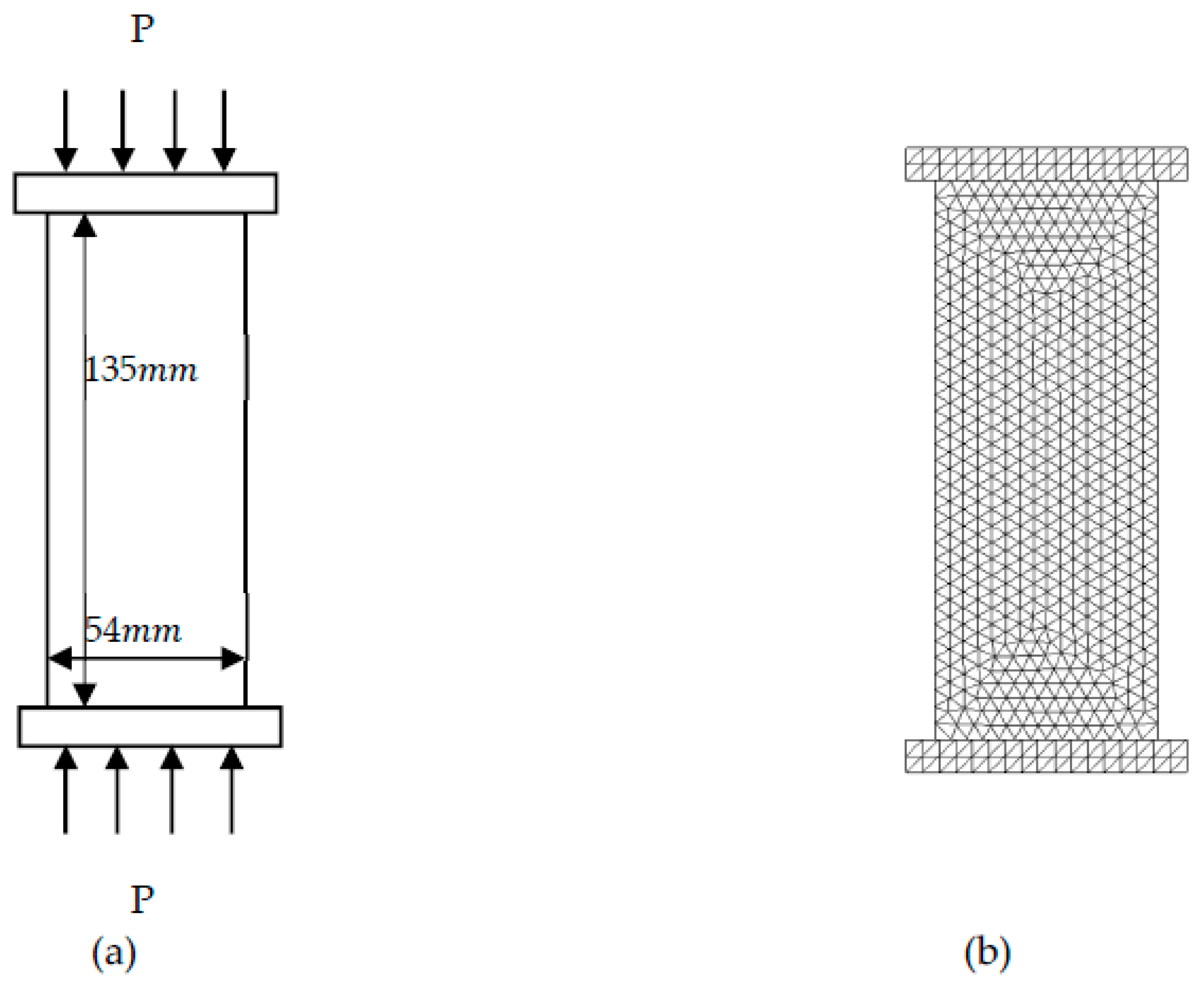
On the basis of the ISRM (1979) [20] suggested method, the geometry of the UCS test is illustrated in Figure 4a. The width of the UCS sample is 54 mm while the length is 135 mm. Figure 4b show the numerical model, which is discretized using three-mode finite elements.

Table 1. Rock properties for the hybrid Finite–discrete models.

Symbols	Properties	Values	Units
$E$	Young’s modulus	60	$\mathrm{GPa}$
$\nu$	Poisson’s ration	0.26	$\mathrm{N}/\mathrm{A}$
$\rho$	Density	2600	${\mathrm{Kgm}}^{-3}$
${\sigma }_t$	Tensile strength	20	$\mathrm{MPa}$
${\sigma }_c$	Compressive Strength	200	$\mathrm{MPa}$
$\varnothing$	Internal friction coefficient	30	°C
$u$	Surface friction coefficient	0.1	$\mathrm{N}/\mathrm{A}$
$G_{fI}$	Mode-I Fracture energy release	50	${\mathrm{Nm}}^{-1}$
$G_{fI}$	Mode-II Fracture energy release	250	${\mathrm{Nm}}^{-1}$

gives the rock parameters. The loading plate properties are tensile strength 100 × 10¹⁶ Mpa, compressive strength 100 × 10¹⁶ Mpa, Young’s modulus 200 Gpa, surface friction coefficient 0.1, and Mode-I and Mode-II fracture energy release 3 × 10¹² ${\mathrm{Nm}}^{-1}$. During the test, the loading rates of 1 m/s is applied on the two loading plates on the vertical direction while the plates are fixed in the horizontal direction. The loading rate, i.e., 1 m/s, is much higher than those in the laboratory test, which is about 0.05 mm/s. The reason to use a high loading rate is to significantly decrease computational time, as the increase in the loading rate can dramatically decrease the computational time. The processor used for the simulation is inter(R) Core (TM) i7-4500U with CPU from 1.80 GHz to 2.40 GHz, while the installed memory (RAM) is 16.0 GB. The system installed in the computer is Windows 8.1 with system type 64-bit Operating System. The current loading rate, i.e., 1 m/s, can reduce at least one order of magnitude in terms of the calculation time compared with loading rate for static tests in laboratory, i.e., around 0.05 m/s.

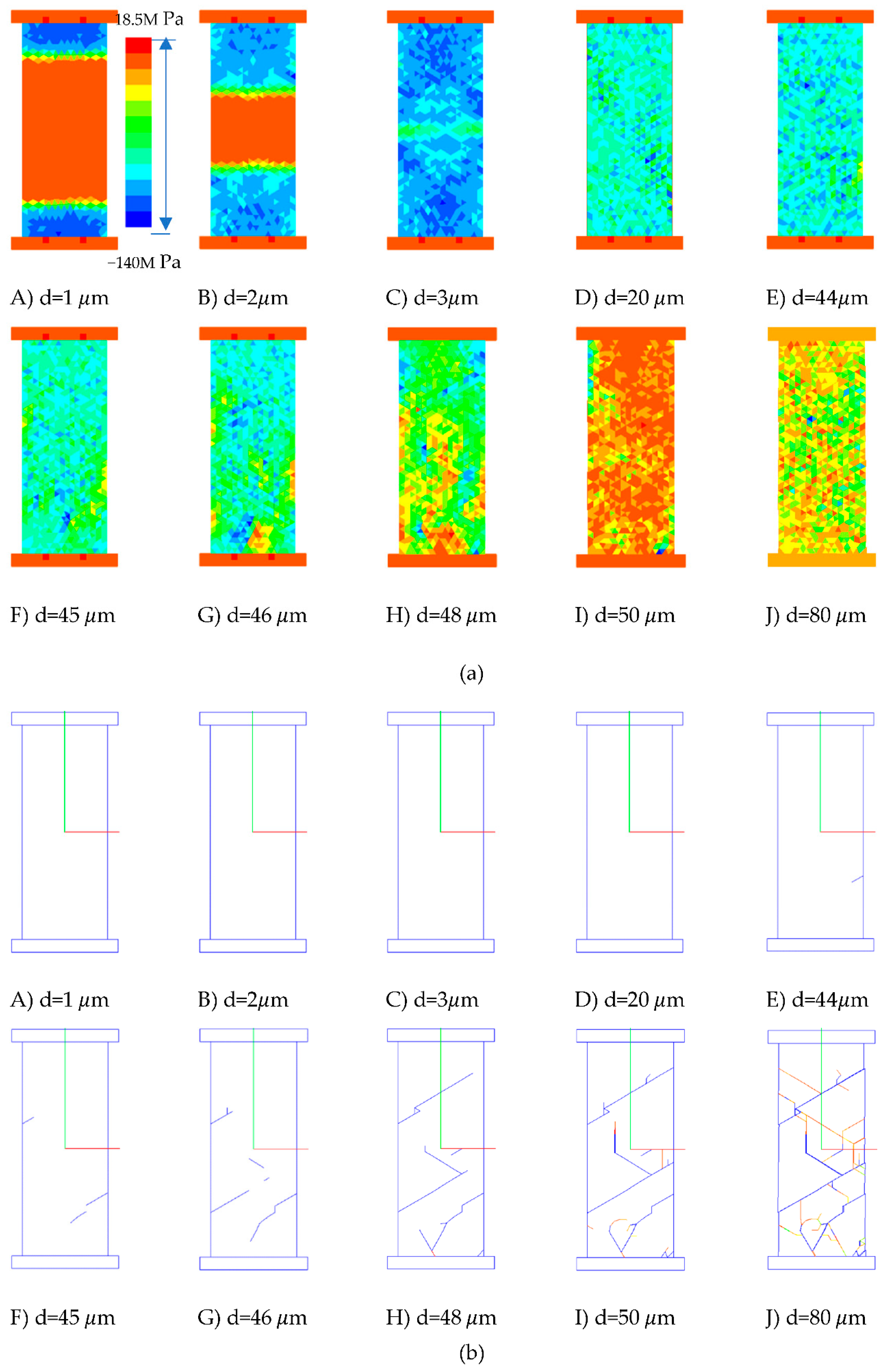
Figure 5 illustrates the fracture process. The red colour indicates the tensile fractures while the blue colour indicates shear fractures.

As the loading plates contact the rock sample, stress concentrations can be observed immediately, as shown in Figure 5a(A). The stresses induced from two sides of the specimen continue to propagate (Figure 5a(B)) when the plate moves. Then, the stresses from the two sides interact (Figure 5a(C)) to form a uniform stress distribution (Figure 5a(D)). The force-loadings increase dramatically and reach their peaks when the plates have moved 44 μm (Figure 6a,b(A–E)). Meanwhile, a small shear crack can be seen in Figure 5b(E). Then, more shear cracks initiate and propagate in the specimen (Figure 5b(F,G)). While the force-loadings drop dramatically (Figure 6a,b(F,I)), two almost parallel shear cracks are produced (Figure 5b(I)). Finally, the force-loadings drop to the bottom (Figure 6a,b(J)). Thus, the rock specimen losses its ability to carry loads, and more cracks are generated, including both shear failure (in blue colour) and tensile failure (Figure 5b(J)).

The uniaxial compressive strength can be calculated as:

$${\sigma }_c=\frac{P_{Max}}{A}=\frac{21.5\times {10}^6}{54\times {10}^{-3}\times 1}=398\mathrm{MPa}$$

(8)

3.2. Numerical Modelling Rock Fracture during BTS Tests

Figure 7a shows the geometrical model for the BTS test, while Figure 7b illustrated the numerical model. For the BTS geometrical model, the diameter is 54 mm. The loading plate moves at the speed of 1 m/s, while the stress is radially applied on the strip with a radian of $2\mathsf{\alpha }$. In the numerical model, the disc is meshed using the three-node finite element. The sample and loading plate parameter are the same as that used for the UCS test. The tensile strength can be obtained according to Equation (9) [21]:

$${\mathsf{\sigma }}_{\mathrm{t}}=\frac{2P}{\pi Dt}$$

(9)

where $P$ is the applied load, $D$ is the diameter, $t$ is specimen thickness.

The analytical solutions for the stress on the vertical diameter can be calculated according to Equations (10) and (11), which are given by Hondros (1959) [22]:

$${\mathsf{\sigma }}_{\mathrm{xx}}=\frac{P}{\pi R\mathrm{t}\mathsf{\alpha }}\left\{\frac{\left[1-{\left(\frac{r}{R}\right)}^2\right]Sin2\mathsf{\alpha }}{1-2{\left(\frac{r}{R}\right)}^{2}Cos2\mathsf{\alpha }+{\left(\frac{r}{R}\right)}^4}-ta{n}^{-1}\left[\frac{1+{\left(\frac{r}{R}\right)}^2}{1-{\left(\frac{r}{R}\right)}^2}tan\left(\mathsf{\alpha }\right)\right]\right\}$$

(10)

$${\mathsf{\sigma }}_{\mathrm{yy}}=-\frac{P}{\pi R\mathrm{t}\mathsf{\alpha }}\left\{\frac{\left[1-{\left(\frac{r}{R}\right)}^2\right]Sin2\mathsf{\alpha }}{1-2{\left(\frac{r}{R}\right)}^{2}Co2\mathsf{\alpha }+{\left(\frac{r}{R}\right)}^4}+ta{n}^{-1}\left[\frac{1+{\left(\frac{r}{R}\right)}^2}{1-{\left(\frac{r}{R}\right)}^2}tan\mathsf{\alpha }\right]\right\}$$

(11)

where $r$, 2$\mathsf{\alpha }$, ${\mathsf{\sigma }}_{\mathrm{xx}}$ and ${\mathsf{\sigma }}_{\mathrm{yy}}$ indicate the means in Figure 7a, i.e., the distance from the disc center, radian, horizontal stress, and vertical stress on the vertical diameter, respectively.

Figure 8a shows the stress propagation process during the BTS test with plates move at 1 m/s. Figure 8b shows the stress fracture evolution process. During the test, high stress is firstly produced from the contact areas (Figure 8a(A)). Then, the two stresses propagate towards the centre of the disc (Figure 8a(B,C)). As shown in the Figure, the forces from the top and bottom plates increases sharply (Figure 9a,b(A–C)). A fracture firstly initiates from the disc’s centre (Figure 8b(C)) and propagates to the disc’s top and bottom (Figure 8b(C)). With the plates moving, the stress is mainly distributed in the centre line of the disc (Figure 8a(D–F)). As the fracture from the centre of the disc reaches the disc top and bottom, shear cracks are observed due to the stress concentrations. After the stress research their peaks, it drops dramatically to the bottom (Figure 9a,b(D–G)), and the disc is separated to two halves (Figure 8b(G)).

$${\mathsf{\sigma }}_{\mathrm{t}1}=\frac{2P_{Max}}{\pi \mathrm{Dt}}=\frac{2\times 2.8698}{3.14\times 0.054\times 1}=34 \mathrm{MPa}$$

(12)

The tensile strength obtained by HFDEM is 34 $\mathrm{MPa}$, while the input value of static tensile strength is 20 $\mathrm{MPa}$. Thus, the HFDEM can well model the strain rate influence on the dynamic strength of rock.

Figure 10 illustrates the stress distribution obtained both by the analytical method and the HFDEM modelling. In addition, the 2P/πDt is used to normalize the stress distribution for better comparison. It can be found from Figure 10 that the HFDEM results agree with the theoretical solution except that the theoretical solution at the loading points is much higher than the modelled result. The reason for having a relatively lower force at the loading points for numerical results maybe because of the tensile and shear failure, which makes the specimen gradually lose its bearing capability.

Figure 11 compares the HFDEM modelled and experimental fracture pattern [23,24]. The two fracture patterns are similar, and they both fracture in the in the vertical direction.

Figure 11c indicates a typical failure pattern for the BTS under loading. It can be seen that the tensile fracture occurs in the vertical diameter, and it separates the sample into two halves, while shear fractures occur at the top and bottom loading contacts due to the compressive stresses concentrating at the contact areas.

To sum up, HFDEM has well modelled the crack process during the BTS test. The main characteristics are captured and show good agreements with typical brittle material under compression. The obtained tensile strength indicates that the HFDEM can capture the effects of the loading rate on rock behaviour.

4. HFDEM Modelling Three Conventional Bending Tests

The HFDEM is used to model the three conventional bending tests in this section to obtain the three fracture models. Figure 12 depicts the geometrical modes for the symmetrical three-point bending (3PB) test, the four-point bending (4PB) test, and the asymmetrical three-point bending (A3PB) test.

The 3PB test, as shown in Figure 12a, is used to obtain the mode-I fracture toughness, and Equation (13) [26] can be used to calculate the values:

$$K_{IC}=\frac{P_{Max}L\sqrt{a}}{B{D}^2}\left[2.9-4.6\left(\frac{a}{D}\right)+21.8{\left(\frac{a}{D}\right)}^2-37.6{\left(\frac{a}{D}\right)}^3+38.7{\left(\frac{a}{D}\right)}^4\right]$$

(13)

In the above equation, $K_{IC}$ indicates the fracture toughness for mode-I fracture, and $P_{Max}$ indicates the peak load. $L$, $a$, B, and D are the distances between the supporting points, notch length, thickness, and width of the beam, respectively.

The 4PB test, as shown in Figure 12b, is used to simulate the shear fracture process and obtain the fracture toughness for mode-II fracture. During the test, two rigid rolls on the top of the beam will move at the same speed for applying loads on the beam. Equation (14) is the analytical solution for mode II fracture toughness [27].

$$K_{IIC}=\frac{P_{Max}}{B\sqrt{D}}\left[\frac{L_2-L_1}{L_2+L_1}\right]\left[1.44-5.08{\left(\frac{a}{D}-0.507\right)}^2\right]\sec \left[\frac{\mathsf{\pi }a}{2D}\right]\sqrt{sin\left[\frac{\pi a}{2D}\right]}$$

(14)

In Equation (14), $K_{IIC}$ and $P_{Max}$ indicate the mode-II fracture toughness and Peak load, respectively. $B$ and D are the thickness and width of the beam, respectively. $L_1$ and $L_2$ are the distances as illustrated in Figure 12. $a$ is the height of the notches as shown in Figure 12.

The A3PB test (Figure 12c) is used to model the fracture process for mixed mode I–II. The fracture toughness for this mixed model can be calculated as follows [28]:

$$K_I=\frac{P_{max}}{B\sqrt{D}}{f}_1\left(a/D,2L_1/L\right)$$

(15)

$$K_{II}=\frac{P_{max}}{B\sqrt{D}}{f}_2\left(a/D,2L_1/L\right)$$

(16)

In Equations (15) and (16), $K_I$ means the mode-I stress intensity factor, and $K_{II}$ indicates the mode-II stress intensity factor. $f_1\left(a/D,2L_1/L\right)$ and $f_2\left(a/D,2L_1/L\right)$ are the coefficients, and in this research, the values are 4.180 and 0.675, respectively.

Figure 13 depicts the numerical modes for the 3PB test, 4PB test, and A3PB test. In Figure 13, triangle elements are employed to discretize the models.

4.1. 3PB Test

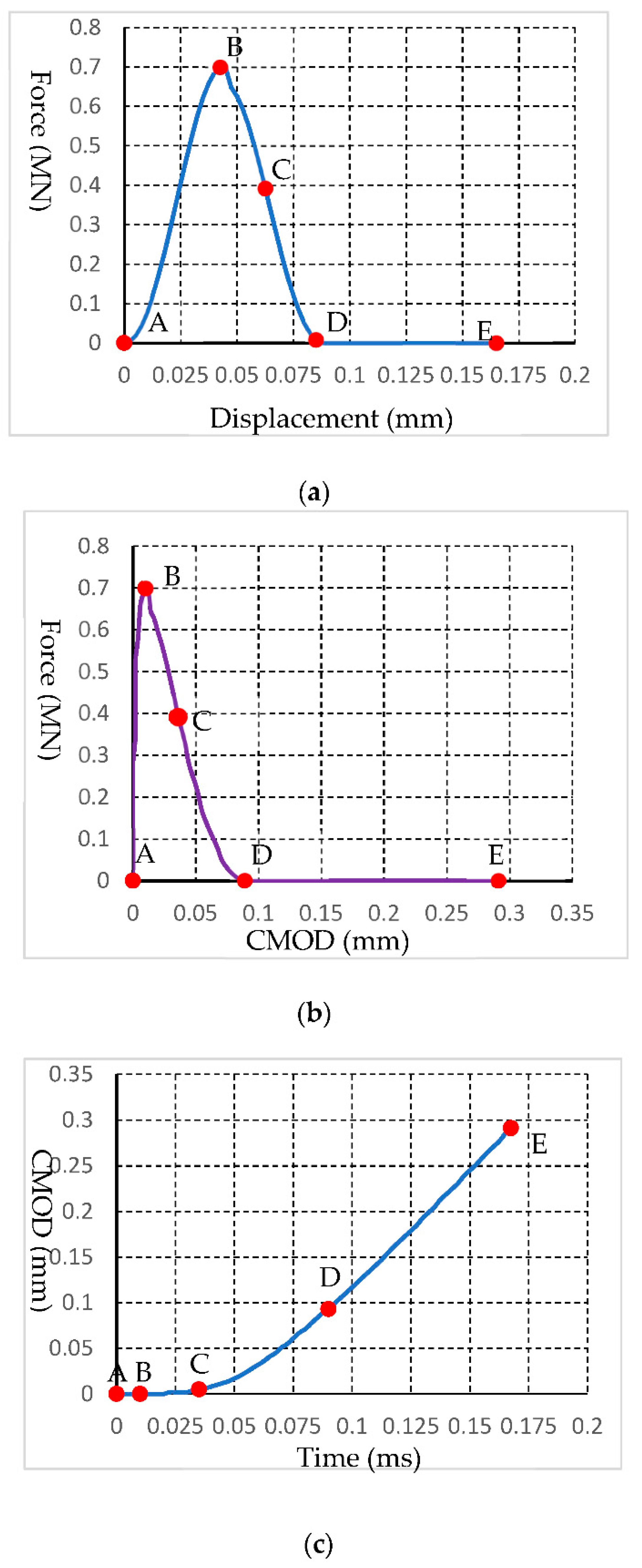
Figure 14 visually tests the 3PB modelling under the loading rates of 1 m/s. Figure 15a illustrates the force-loading displacement curves. Figure 15b shows the force-loading crack mount opening displacement (CMOD) curve, while Figure 15b(C) depicts the CMOD time curve. The letters marked on Figure 15 are from Figure 14.

During the tests, the loading rate on the top of the beam moves at 1m/s for the models of the three types of fracture, i.e., tensile, shear, and mixed fractures.

The stress is produced immediately (Figure 15a(A,B)) as the top roll moves. Meanwhile, a crack starts to propagate from the original notch in the beam (Figure 14B). With the moving of the rigid roll, the force continues to increase and finally reaches Point B (Figure 15a(B)). Then, the force begins to drop quickly while the crack from the tip of notch continue to propagate. The Figure 15c(B,C) illustrates that the CMOD continues to increase while the force continues to drop (Figure 15a(B,C)). In the end, the beam is separated into two halves (Figure 14E).

The FDEM modelled 3PB test agree with the literature [29,30] in terms of the fracture propagation process and fracture patterns. The force-loading CMOD curve obtained by FDEM (Figure 15b) show the same characteristic as recorded in the literature [29].

The fracture toughness for mode-I obtained using HFDEM modelling 3PB test can be calculated using Equation (17):

$$K_{IC1}=\frac{697.71\times 3.33\times 54\sqrt{0.4\times 54\times {10}^{-3}}}{1\times {54}^2}\left[2.9-4.6\times 0.4+21.8\times {0.4}^2-37.6\times {0.4}^3+38.7\times {0.4}^4\right]=19.48 \mathrm{MPa}\sqrt{m}$$

(17)

4.2. Four-Point Bending Test (Pure Mode-II Fracture)

Figure 16 visually shows the HFDEM modelling 4PB test. The loading rate of 1m/s for the two rigid roll is applied on top of the beam. The curve illustrating the relationship between loading force and the displacement is recorded in Figure 17a, while the relationships between the force-loading and the crack mouth opening/sliding displacements are shown in Figure 17b,c. In Figure 17, the curves are marked using alphabets, which referee to those in Figure 16.

Initially, a notch is placed in the middle of the bottom beam (Figure 16A). As the top roll moves downwards and contact the beam, a force is induced immediately and increases rapidly, although there is a fluctuation (Figure 17a(A,B)). The pre-fabricated notch is slightly opened (Figure 17b(A,B)) while almost no sliding occurs (Figure 17c(A,B)). Then, a crack firstly occurs at the tip of the notch, and it propagates towards the left loading point (Figure 16B). Due to the crack initiated from the prefabricated notch, the force suddenly drops (Figure 17a(A,B)). However, the beam does not completely lose its ability to carry loads. As the top roll moves, the force continually increases (Figure 17a(B,C)). While the crack continues to propagate, a new crack at the top of the beam between the two loading points is induced (Figure 16C). As the two cracks propagate (Figure 16D), the force rapidly increases to its peak (Figure 17a(D)). Meanwhile, the CMOD and CMSD are both increased (Figure 17b,c(B–D)). Then, the force-loading begins to drop quickly (Figure 17a(D,E)) as the crack induced from the tip of notch reaches the left loading point (Figure 16E). Finally, the opening and sliding distances of the crack mouth reach their maximums (Figure 17a(E,F)).

There are two peaks on the force loading–displacement curves. When the crack starts to occur from the tip of the notch, the stress reaches its first peak. Thus, the first peak stress is used to obtain the fracture toughness for mode-II fracture according to Equation (18):

$$K_{IIC1}=\frac{1.21MN}{B\sqrt{D}}\left[\frac{L_2-L_1}{L_2+L_1}\right]\left[1.44-5.08{\left(\frac{a}{D}-0.507\right)}^2\right]\sec \left[\frac{\mathsf{\pi }a}{2D}\right]\sqrt{sin\left[\frac{\pi a}{2D}\right]}=4.979\mathrm{Mpa}\sqrt{m}$$

(18)

4.3. Asymmetrical Three-Point Bending Test (Mixed-Mode I–II Fracture)

Figure 18 depicts the fracture initiation and propagation process for A3PB, while Figure 19 shows the relationship between the force loading and the displacement. When the loading rolls contact the beam, compressive stresses are produced immediately and increase quickly to their peaks (Figure 19A,B). During this period, no cracks occur in the beam (Figure 18A,B). Then, a crack is produced at the tip of the notch (Figure 18B). As the force loading continues to decrease (Figure 18B–D), a tensile crack is observed at the bottom.

At the end, the crack from the middle of the bottom beam first reaches the top loading point while the crack from the notch reaches the top beam boundary. According to the colour indication, the crack from the bottom of beam is mainly tensile failure while the crack from the prefabricated notch is mixed by tensile and shear failures. Finally, the beam is divided into two parts by the tensile failure at the middle of the beam (Figure 18F) and the force disappears (Figure 18E,F).

According to the peak force (Figure 19), the fracture toughness for pure mode-I and mode-II can be calculated using Equations (19) and (20), respectively:

$$K_I=\frac{P_{max}}{B\sqrt{D}}{f}_1\left(a/D,2L_1/L\right)=15.29 \mathrm{MPa}\sqrt{m}$$

(19)

$$K_{II}=\frac{P_{max}}{B\sqrt{D}}{f}_2\left(a/D,2L_1/L\right)$$

(20)

Figure 20 illustrates the force-loading CMOD/CMSD curves for the A3PB test. The alphabet in Figure 20 corresponds to those in Figure 18. Before 0.022 ms, there is no displacement or sliding at the notch tip according to Figure 20. After that, the CMOD and CMSD begins to increase. According to Figure 19, at point B, the force loading reaches its peak, and the crack occurs. Then, the CMOD and CMSD continue to propagate (Figure 20C–E) while the force loading drops dramatically (Figure 20C–E). Finally, as the crack reaches top boundary (Figure 18F), the CMOD and CMSD reach their maximum (Figure 20F).

5. Discussion

5.1. Effect of the Strain Rate Rock Strength

To compare the influence of the loading rate, the increasing factor of dynamic strength (DIF) is employed herein. The DIFs obtained from the HFDEM modelling of the of BTS tests. Figure 21 shows the comparison between the HFDEM obtained DIF with those obtained from literatures.

As shown in Figure 21, the DIFs increase with the strain rate increasing before the strain rate increases to a certain threshold, i.e., 10/s. After the threshold, the rock strengths increase with the strain rate increasing dramatically. As can be seen for the rock strength obtained from the BTS test by the hybrid method, the increasing trends are the same with those obtained from literature. Thus, the HFDEM can reflect the influence of the strain on the dynamic rock strength.

5.2. Loaidng Rate Influence on Rock Toughness

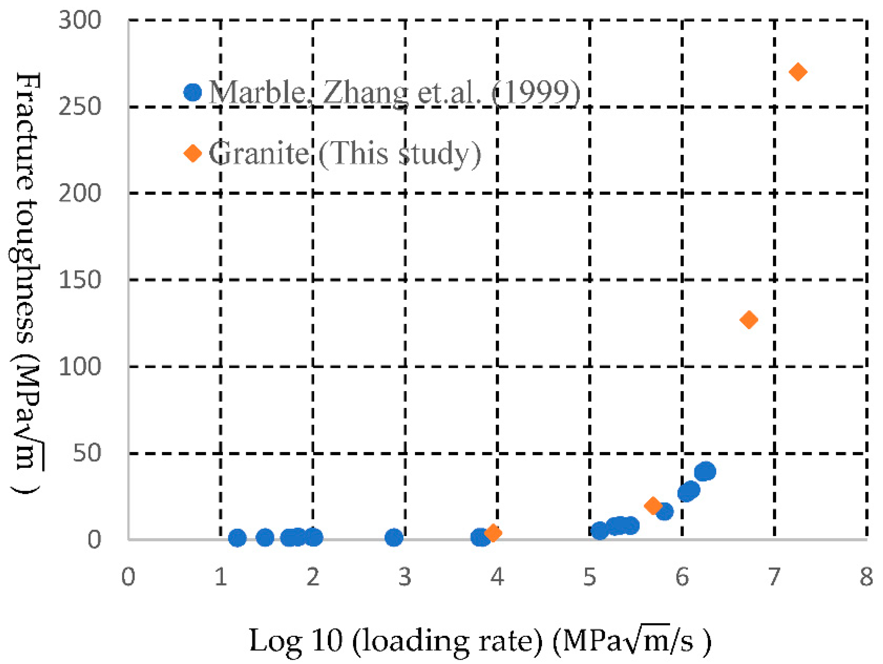
In this section, the loading rate influences on the fracture toughness are studied. Figure 22 illustrates the relationship between the loading rate and the fracture toughness.

One group of the results is from the experimental study [33], while the group of the research is from this study. The fracture toughness is not influenced by the loading rate while the loading rate is smaller than a certain threshold, i.e., ${10}^5\mathrm{MPa}\sqrt{m}$/s. After that, the dynamic fracture toughness is obviously related to the the loading rate, and the dynamic fracture dramatically increases with the loading rate. The obtained fracture toughness shows the same characters as shoes in literature as shown in Figure 22. Thus, the HFDEM can capture the rock fracture characters.

5.3. Effect of the Mesh Orientation

In the HFDEM, the fracturing of the rock is modelled through the separation of the adjunct finite element in the form of opening or sliding. Thus, the orientation and size of the discretized meshes will definitely affect the fracture pattern.

To illustrate the effect the mesh size, the UCS test model is meshed using structural meshes and modelled by the hybrid method to compare with the modelled result with free meshes. Figure 23 shows the UCS test mode with structural mesh, while Figure 24 indicates the modelled results

Initially, a shear fracture occurs at the bottom of the sample as shown in Figure 24B. Then, the crack propagates linearly to the right side of the model as illustrated in Figure 24C. Thus, the specimen is separated into two parts. After that, the two parts of the specimen slide along the new formed shear cracks (Figure 24E). Compared with the modelled result using free mesh in Figure 5, both modelled results have the same characteristics in general, i.e., inclined cracks separating the specimen. However, the fracture patterns are not exactly the same. The size and orientation of the mesh can obviously affect the fracture patterns.

6. Conclusions

This research briefly reviews the numerical method based on their material hypothesis. Among all types of numerical method, the HFDEM is proposed to model the different fracture modes using three conventional point bending tests. Three fracture modes and strain rate effects are taken into account in the HFDEM. Then, the HFDEM is calibrated by modelling UCS and BTS tests. The modelled fracture patterns are similar to experimental results, and the obtained rock strength indicates that the HFDEM can reflect the influence of strain rate. Then, the HFDEM is used to model three conventional bending tests. The various fracture types are modelled, and the corresponding fracture toughness are obtained. It is found that:

The HFDEM is able to simulate various fracture types by the implementation of three fracture modes.

The HFDEM can capture the influence of the strain rate on rock behaviours such as the static and dynamic strength relationships implemented in the HFDEM.

The FDEM is a useful numerical technique for rock engineering since it can simulate the complete rock fracture process and take the influence of the strain rate into account.

References

- Donzé, F.V.; Richefeu, V.; Magnier, S.-A. Advances in discrete element method applied to soil, rock and concrete mechanics. State of the art of geotechnical engineering. Electron. J. Geotech. Eng. 2009, 44, 31. [Google Scholar]
- Cundall, P.A. A computer model for simulating progressive, large-scale movement in blocky rock systems. Proc. Symp. Int. Soc. Rock Mech. 1971. Available online: https://www.scienceopen.com/document?vid=838c3a34-fe64-4dc6-8d2b-e9aee0c5b466 (accessed on 19 October 2021).
- Lisjak, A.; Grasselli, G. A review of discrete modeling techniques for fracturing processes in discontinuous rock masses. J. Rock Mech. Geotech. Eng. 2014, 6, 301–314. [Google Scholar] [CrossRef] [Green Version]
- Mayer, J.M.; Stead, D. Exploration into the causes of uncertainty in UDEC Grain Boundary Models. Comput. Geotech. 2017, 82, 110–123. [Google Scholar] [CrossRef]
- Aliabadian, Z.; Sharafisafa, M.; Nazemi, M.; Khameneh, A.R.; Kazerani, T. Discrete element modeling of wave and fracture propagation in delay time breakage. Rock Dyn. Appl. State Art 2013, 7, 401–407. [Google Scholar]
- Gutiérrez-Ch, J.G.; Senent, S.; Melentijevic, S.; Jimenez, R. Distinct element method simulations of rock-concrete interfaces under different boundary conditions. Eng. Geol. 2018, 240, 123–139. [Google Scholar] [CrossRef]
- Gutiérrez-Ch, J.G.; Senent, S.; Estebanez, E.; Jimenez, R. Discrete element modelling of rock creep behaviour using rate process theory. Can. Geotech. J. 2021, 58, 1231–1246. [Google Scholar] [CrossRef]
- Jing, L. A review of techniques, advances and outstanding issues in numerical modelling for rock mechanics and rock engi-neering. Int. J. Rock Mech. Min. Sci. 2003, 40, 283–353. [Google Scholar] [CrossRef]
- Jing, L.; Hudson, J.A. Numerical methods in rock mechanics. Int. J. Rock Mech. Min. Sci. 2002, 39, 409–427. [Google Scholar] [CrossRef]
- Board, M. UDEC (Universal Distinct Element Code) Version ICG1. 5; NUREG/CR-5429-Vol.2; Itasca Consulting Group, Inc.: Minneapolis, MN, USA, September 1989. [Google Scholar]
- Cundall, P.A.; Strack, O.D.L. The Distinct Element Method as a Tool for Research in Granular Material; University of Minnesota: Minneapolis, MN, USA, 1978. [Google Scholar]
- Shi, G.H.; Goodman, R.E. Two dimensional discontinuous deformation analysis. Int. J. Numer. Anal. Methods Geomech. 1985, 9, 541–556. [Google Scholar] [CrossRef]
- Lin, C.T.; Amadei, B.; Jung, J.; Dwyer, J. Extensions of discontinuous deformation analysis for jointed rock masses. Int. J. Rock Mech. Min. Sci. Geomech. Abstr. 1996, 33, 671–694. [Google Scholar] [CrossRef]
- Fukuda, D.; Mohammadnejad, M.; Liu, H.; Dehkhoda, S.; Chan, A.; Cho, S.; Min, G.; Han, H.; Kodama, J.; Fujii, Y. Development of a GPGPU-parallelized hybrid finite-discrete element method for modeling rock fracture. Int. J. Numer. Anal. Methods Geomech. 2019, 43, 1797–1824. [Google Scholar] [CrossRef]
- Munjiza, A.A. The Combined Finite-Discrete Element Method; John Wiley & Sons Ltd.: Chichester, UK, 2004. [Google Scholar]
- An, H.; Liu, H.; Han, H.; Zheng, X.; Wang, X. Hybrid finite-discrete element modelling of dynamic fracture and resultant fragment casting and muck-piling by rock blast. Comput. Geotech. 2017, 81, 322–345. [Google Scholar] [CrossRef]
- Mahabadi, O.K.; Grasselli, G.; Munjiza, A. Y-GUI: A graphical user interface and pre-processor for the combined finite-discrete element code, Y2D, incorporating material heterogeneity. Comput. Geosci. 2010, 36, 241–252. [Google Scholar] [CrossRef]
- Liu, H.; Kou, S.; Lindqvist, P.-A.; Tang, C. Numerical studies on the failure process and associated microseismicity in rock under triaxial compression. Tectonophysics 2004, 384, 149–174. [Google Scholar] [CrossRef]
- Zhao, J. Applicability of Mohr–Coulomb and Hoek–Brown strength criteria to the dynamic strength of brittle rock. Int. J. Rock Mech. Min. Sci. 2000, 37, 1115–1121. [Google Scholar] [CrossRef]
- Bieniawski, Z.T.; Bernede, M.J. Suggested methods for determining the uniaxial compressive strength and deformability of rock materials: Part 1. Suggested method for determination of the uniaxial compressive strength of rock materials. Int. J. Rock Mech. Min. Sci. Geomech. Abstr. 1979, 16, 137. [Google Scholar] [CrossRef]
- Timoshenko, S.P.; Goodier, J.N. Theory of Elasticity; McGraw-Hill: New York, NY, USA, 1970. [Google Scholar]
- Hondros, G. The evaluation of Poisson’s ratio and the modulus of materials of a low tensile resistance by the Brazilian (indirect tensile) test with particular reference to concrete. Aust. J. Appl. Sci. 1959, 10, 243–268. [Google Scholar]
- Li, D.; Wong, L.N.Y. The Brazilian disc test for rock mechanics applications: Review and new insights. Rock Mech. Rock Eng. 2013, 46, 269–287. [Google Scholar] [CrossRef]
- Hobbs, D.W. The tensile strength of rocks. Int. J. Rock Mech. Min. Sci. Geomech. Abstracts. 1964, 1, 385–396. [Google Scholar] [CrossRef]
- An, H.; Liu, H.; Wang, X.; Shi, J.; Han, H. Hybrid continuum-discontinuum modelling of rock fracutre process in Brazilian tensile strength test. Civ. Eng. J. 2017, 26, 237–249. [Google Scholar] [CrossRef]
- Brown, W.F.; Srawley, J.E. Plain Strain Fracture Toughness Testing of High Strength Metallic Materials; ASTM International: West Conshohocken, PA, USA, 1966. [Google Scholar]
- Rao, Q. Pure Shear Fracture of Brittle Rock-A Theoretical and Laboratory Study. Ph.D. Thesis, Luleå University of Technology, Luleå, Sweden, 1999. [Google Scholar]
- Whittaker, B.N.; Singh, R.N.; Sun, G. Rock Fracture Mechanics: Principles, Design, and Applications; Elsevier: Amsterdam, The Netherlands, 1992. [Google Scholar]
- Zhou, X.-P.; Qian, Q.-H.; Yang, H.-Q. Effect of loading rate on fracture characteristics of rock. J. Cent. South Univ. Technol. 2010, 17, 150–155. [Google Scholar] [CrossRef]
- Liu, H.Y.; Kou, S.Q.; Lindqvist, P.-A.; Tang, C.A. Numerical Modelling of the Heterogeneous Rock Fracture Process Using Various Test Techniques. Rock Mech. Rock Eng. 2006, 40, 107–144. [Google Scholar] [CrossRef]
- Asprone, D.; Cadoni, E.; Prota, A. Experimental analysis on tensile dynamic behavior of existing concrete under high strain rates. ACI Struct. J. 2009, 106, 106–113. [Google Scholar]
- Cho, S.H.; Ogata, Y.; Kaneko, K. Strain-rate dependency of the dynamic tensile strength of rock. Int. J. Rock Mech. Min. Sci. 2003, 40, 763–777. [Google Scholar] [CrossRef]
- Zhang, Z.X.; Kou, S.Q.; Yu, J.; Yu, Y.; Jiang, L.G.; Lindqvist, P.-A. Effects of loading rate on rock fracture. Int. J. Rock Mech. Min. Sci. 1999, 36, 597–611. [Google Scholar] [CrossRef]
Figure 1.
Typical brittle material stress–strain curve. , , , represent the stress loading, peak stress, strain, and peak strain, respectively.
Figure 2.
Hybrid Finite–discrete fracture model (red line represents edges of joint elements while the black line represents the edge of the finite elements): (a) Without stress; (b) Under tension condition; (c) Under shear condition; (d) Under both tension and shear condition.
Figure 3.
Bonding stress and opening or sliding displacement: (a) Mode-I; (b) Mode-II; (c) Mixed mode I–II.
Figure 4.
Geometrical and numerical model of uniaxial compression test: (a) Geometrical model; (b) Numerical model.
Figure 5.
HFDEM modelling UCS test: (a) Minor principal stress; (b) fracture process.
Figure 6.
HFDEM obtained curves during the UCS test: (a) Top plate force; (b) Bottom plate force.
Figure 7.
HFDEM model for BTS test: (a) Geometrical model; (b) Numerical model.
Figure 8.
HFDEM modelling of Brazilian tensile strength tests: (a) Minor principal stress; (b) fracture propagation; (A) d = 1m; (B) d = m; (C) d = m; (D) d = m; (E) d = m; (F) d = m; (G) d = m.
Figure 9.
HFDEM obtained curves during BTS test: (a) force from the top plate; (b) force from the bottom plate.
Figure 10.
Comparison of the HFDEM obtained results with analytical solutions in terms of stress distribution.
Figure 11.
Comparison of HFDEM result with results from the literature: (
a) HFDEM result; (
b) experimental result [
25]; (
c) Typical rock failure pattern [
23,
24].
Figure 12.
Geometrical mode for 3PB and 4PB tests: (a) 3PB test; (b) 4PB test; (c) Asymmetrical A3PB test.
Figure 13.
Numerical model for 3PB and 4PB tests: (a) 3PB or A3PB tests models; (b) 4PB test.
Figure 14.
HFDEM modelling rock failure processes in 3PB test. (A) Initial state; (B) Crack initation; (C) Crack propagation; (D) Crack continual propagation; (E) Crack completion.
Figure 15.
Curves for force-loading with displacement, CMOD, and Time during 3PB test: (a) Force-loading displacement curve; (b) Force-loading CMOD curve; (c) Force-loading CMOD curve.
Figure 16.
Crack initiation and propagation of 4PB test.
Figure 17.
Force loading related curves for 4PB test: (a) Force-loading displacement curve; (b) Force-loading CMOD curve; (c) Force-loading CMSD curve.
Figure 18.
Fracture initiation and propagation for A3PB test.
Figure 19.
Force-loading displacement for A3PB test.
Figure 20.
Force-loading CMOD/CMSD curves for A3PB test under the loading rate of 1 m/s.
Figure 21.
DIFs obtained from HFDEM modelling and literature [
31,
32].
Figure 22.
The modelled result and the experimental results [
33] comparison t in terms of relationship between the fracture toughness (mode-I) and loading rate.
Figure 23.
Structural meshed UCS test model.
Figure 24.
HFDEM modelling fracture process of UCS test.