Assessing the Impact of Fossil Fuel Prices on Renewable Energy in China Using the Novel Dynamic ARDL Simulations Approach

Abstract

The past few decades have been marked by a gradual but steady increase in the reliance on renewable energy. In this study, we examined whether the prices of fossil fuels, namely, oil, coal, and natural gas, have affected renewable energy consumption in China during the period 1980–2018. To this end, we employed the novel dynamic Autoregressive Distributed Lag simulations approach. In the light of the empirical investigation, some intriguing conclusions have been drawn. We found strong evidence of the cointegrating relationship between the prices of all fossil fuels and renewable energy consumption. Furthermore, rising oil, coal, and natural gas prices resulted in increased renewable energy consumption in the long run, confirming that renewable energy sources can substitute fossil fuel energy only in the long run. Nevertheless, there is no evidence of significant effects in the short run. When considering the presence of structural breaks, the findings confirm the robustness of the dynamic ARDL simulations, as we conclude that fossil fuel prices positively affect renewable energy consumption only in the long run.

1. Introduction

Policy makers and academics have agreed that the unprecedented climate change has severely affected environmental quality and public health. The exponential growth in carbon dioxide emissions due to the extensive use of fossil fuel energy is recognized as the primary source of environmental degradation. According to British Petroleum [1], global direct primary energy consumption has risen substantially during the past few decades. Fossil fuels remain the primary energy source. More specifically, oil represented about 31% of primary energy consumption in 2019, while coal and natural gas shares were about 25.3% and 22.7%, respectively. The increase in fossil fuel consumption due to the dependence of some economies on these traditional energy sources has caused harmful effects on environmental quality. In reaction to this situation, the United Nations Framework Convention on Climate Change initiated the Paris Agreement signed in 2015. It was suggested, among other things, that the transition from non-renewable to renewable energy be accelerated. The question of whether renewable energy sources could be suitable substitutes for traditional energy sources has arisen. Such a situation was also exacerbated by the fact that forecasting fossil fuel prices has become challenging in recent years, putting both customers and producers at risk of price fluctuations.

In the past few decades, there has been a growing body of literature analyzing factors affecting the development of clean energy [2,3,4]. Among others, the impact of fossil fuel prices on renewable energy has been examined by many scholars, such as Murshed and Tanha [5], Zhao et al. [6], Brini et al. [7], and Apergis and Payne [8,9,10]. Two main conclusions may be derived when reviewing the literature on this subject. The first is that almost all studies have examined the impact of oil prices on renewable energy. The effects of other fossil fuel energy sources, such as natural gas and coal, have been ignored. The second statement is the inconclusive and mixed results reached by prior studies. For instance, substantial research highlighted the favorable effect of oil prices on renewable energy [6,7,8,9,10]. Far fewer studies conclude that the linkage between oil prices and renewable energy is negative [11]. Finally, scarce literature argues that the outcomes of oil prices on renewable energy may be nonlinear, suggesting an optimal threshold level [4].

Using data covering the period 1980–2018, we aimed to examine the effects of fossil fuel prices on renewable energy consumption in China. Unlike most previous literature, we considered all types of fossil fuels, namely, oil, coal, and natural gas. China is considered an appropriate case study for several reasons. First, China’s economy relies significantly on fossil fuel energy sources, which provided more than 85% of total primary energy consumption in 2019.

Table A1. Energy, environmental and economic statistics in the most-polluting countries.

	CO2 Emissions		Non-Renewable Energy Consumption		Renewable Energy Consumption		GDP
	Value	Share	Value	Share	Value	Share	Value	Share
China	9810.456	28.5%	120.825	24.6%	6.750	23.4%	$1.43\times {10}^{13}$	16.9%
U.S.	5029.389	14.6%	79.046	16.1%	5.709	19.8%	$1.99\times {10}^{13}$	23.5%
India	2471.946	7.2%	30.718	6.2%	1.326	4.6%	$2.69\times {10}^{12}$	3.2%
Russia	1595.685	4.6%	26.278	5.3%	0.021	0.07%	$1.46\times {10}^{12}$	1.7%
Japan	1117.672	3.2%	16.119	3.3%	1.008	3.5%	$4.57\times {10}^{12}$	5.4%

Notes: Values are expressed in million tonnes of carbon dioxide (CO₂ emissions), constant 2015 USD (GDP), exajoules (non-renewable and renewable energy consumption), while share represents the proportion of a given country in the world. Data are from bp Statistical Review of World Energy July 2021 and World Development Indicators.

in the Appendix A suggests that 24.6% of global fossil fuel energy and 23.4% of renewable energy are consumed by China. A worldwide overview leads us to consider China as the largest consumer of coal. According to the China National Coal Association, the demand for coal was about 2500 megatons in 2008 and increased to about 4000 megatons in 2020. China is also considered the largest importer of oil. The fact that China surpassed the United States in terms of annual total crude oil imports characterized 2017 as a watershed moment. Regarding natural gas, China is ranked third globally, accounting for around 6.4% of worldwide natural gas consumption. Second, China has long been considered the world’s largest contributing country to CO₂ emissions, owing to its massive use of fossil fuel energy sources, particularly coal. Indeed, China accounted for around 28% of global CO₂ emissions in 2019, surpassing the developed world [12].

This research adds to the current literature in various ways. First, it is among a handful of empirical studies that analyze the effects of all fossil fuel prices (oil, coal, and natural gas) on renewables. The majority of previous research concentrated exclusively on the impact of oil prices. Second, unlike previous studies that have relied on conventional econometric techniques to check the presence of cointegration, we employed the novel dynamic Autoregressive Distributed Lag simulations approach proposed by Philips [13] and Jordan and Philips [14]. According to Abbasi et al. [15], this method avoids problems when estimating short- and long-run effects using the conventional ARDL approach developed by Pesaran et al. [16]. The dynamic ARDL also allows predicting, stimulating, and plotting the effects of a counterfactual change in the explanatory variable on the dependent variable. Third, the empirical analysis considers the potential presence of structural breaks in the data when estimating the impact of fossil fuel prices on renewable energy. To deal with this issue, we identify the dates of breakpoints using the Bai and Perron [17,18] multiple breakpoint test.

The remainder of this research is structured as follows. The existing literature is presented in Section 2, while Section 3 details the data and econometric methodology. The empirical results are discussed in Section 4, while Section 5 is reserved for the conclusion.

2. Literature Review

In the past two decades, increasing concerns about climate change, energy security, and environmental quality have urged academicians and policy makers to rethink the use of traditional fossil energy. There has been a consensus that renewable energy development has become an overriding objective. As Büyüközkan and Güleryüz [19] pointed out, renewable energy sources have received much interest from investors as a green alternative to traditional fossil energy.

The existing literature has well documented the main drivers of renewable energy. Regarding this issue, Marques et al. [20] emphasized that renewable energy determinants may be divided into three categories, socioeconomic, political, and country-specific factors. Aguirre and Ibikunle [21] examined factors affecting renewable energy investment in 38 economies from 1990 to 2010. According to the findings, specific energy regulations hinder renewable energy investment. In their work, Damette and Marques [22] identified a positive association between national revenues and energy consumption on the one hand and renewable energy on the other hand. Kumar et al. [23] examined whether renewable and non-renewable energy sources are substitutes or complements. To this end, the authors used a sample of 12 OECD countries over the period 1995–2009. The empirical results confirm the validity of the two hypotheses. Indeed, non-renewable energy is shown to complement renewable energy in eight countries while substituting it in four others. Other studies have associated renewable energy with economic globalization and technological progress. Using a sample of 30 OECD nations from 1970 to 2015, Gozgor et al. [24] explored the response of renewable energy to economic globalization. The findings show that a more globalized economy promotes the development of the renewable energy industry. Moreover, Padhan et al. [25] examined the relationship between renewable energy use and globalization in OECD countries. Overall, it has been reported that increased globalization stimulates renewable energy consumption. Bamati and Raoofi [26] investigated the aforementioned relationship in 25 countries from 1990 to 2015. According to the Generalized Least Squares estimator, technological exports considerably increase renewable energy production only in developed countries, whereas no significant effect was found in developing countries. Similar impacts were also reported for the two groups of countries in terms of GDP per capita and oil prices.

Previous studies have also discussed the role of oil price fluctuations as a driver of renewable energy. Zhao et al. [6] developed a general equilibrium model to investigate the outcomes of international oil price fluctuations on renewable energy development and investment in China. The results suggest that an increase in oil prices stimulates investment in renewable energy. The Russian context was analyzed by Karacan et al. [11]. The authors used data from 1990 to 2015 to investigate the linkage between CO₂ emissions, income, oil prices, and renewable energy. Contrary to expectations, the Vector Error Correction model suggests a negative linkage between oil prices and renewable energy. Using data over the period 1980–2011, Brini et al. [7] focused on the linkages between energy consumption, trade, oil prices, and output in Tunisia. The empirical evidence suggests that when oil costs rise, so does renewable energy use. In addition, unidirectional short-run causality between the two variables is confirmed. Apergis and Payne [8] studied the causal linkages between economic growth, CO₂ emissions, oil prices, and renewable energy. To this end, they used a sample of 25 OECD countries from 1980 to 2011. The panel cointegration results support the presence of a long-run relationship between variables. More specifically, findings reveal that renewable energy, economic growth, CO₂ emissions, and oil prices all have a positive and significant relationship. In other work, Apergis and Payne [10] investigated the same relationship in 11 South American countries between 1980 and 2010. The authors conclude that the long-run association between carbon dioxide emissions, oil prices, economic growth, and renewable energy is positive and statistically significant.

Apergis and Payne [9] examined the nonlinear association between renewable energy, economic growth, CO₂ emissions, and fossil fuel (oil and coal) prices in Central America using the Panel Smooth Transition Regression model. Their findings confirmed the presence of long-run relationships between the considered variables. Additionally, the fully modified ordinary least squares revealed positive and significant effects of oil and coal prices on renewable energy. Murshed and Tanha [5] recently analyzed the impact of oil price shocks on renewable energy in selected South Asian net oil-importing countries from 1990 to 2018. The long-run analysis revealed a nonlinear relationship, suggesting that an increase in oil prices initially impedes renewable energy use. Then, overcoming a specific threshold, further increases in oil prices enhance renewable energy consumption. Guo et al. [27] explored the asymmetric effects of oil prices on renewable energy in G7 countries based on the linear and nonlinear ARDL models. Their findings indicate significant asymmetric impacts of oil prices on renewable energy use in all countries except France and Germany. Li and Leung [28] considered the coal and natural gas prices when analyzing the linkages between economic growth and renewable energy consumption in selected European countries from 1985 to 2018. The Pooled Mean Group estimator suggests that coal and natural gas prices positively affect long-term renewable energy consumption.

3. Materials and Methods

We sought to examine the effects of fossil fuel prices on renewable energy use in China from 1980 to 2018. Unlike most previous works, the current study considers all types of fossil fuels. The effects of crude oil, coal, and natural gas prices on renewable energy use are particularly analyzed in this research. Data on fossil fuel prices were obtained from the World Bank Commodity Price Data dataset compiled by the World Bank. The oil price is measured by the real average crude oil price, which includes Dubai, Brent, and WTI crude oil prices, whereas the annual real coal price represents the coal price. Finally, natural gas price is measured by the natural gas index, which is the average of natural gas prices in Europe, the U.S., and Japan. The dependent variable, renewable energy consumption, is provided by the U.S. Energy Information Administration and is expressed in million tons of oil equivalent. The empirical model also includes a set of control variables. As in Bamati and Raoofi [26], we include the real GDP expressed in U.S. dollars since countries with higher income are more likely to implement renewable energy projects and have more access to technological innovations that promote renewable energy development. Foreign direct investments as a share of GDP are also introduced in the model since foreign investors are seen as a source of knowledge transfer that may promote energy efficiency through renewable energy development [29]. Data relative to these two variables were obtained from the World Development Indicators. Moreover, we introduce a variable on the patents on environmental technologies to check how innovation affects renewable energy consumption. The corresponding data were extracted from the Organization for Economic Co-operation and Development dataset. Finally, a variable measuring the level of carbon dioxide emissions is included, as environmental degradation may induce a shift toward more clean energy sources. This variable is especially relevant for China, the most polluting country in the world. Data on annual CO₂ emissions were obtained from BP Statistical Review of World Energy June 2020. To give the data series a constant variance, we used the logarithmic transformation of all variables.

The empirical analysis was carried out in different stages. We started by checking the properties of the data, particularly the stationarity. Indeed, both the conventional and dynamic ARDL models require I (0) or I (1) variables, as well as a strictly I (1) dependent variable [30,31,32]. To this end, we implemented the ADF unit root test with bootstrapped critical values. We conducted 10,000 bootstrap replicates to simulate critical values. The unit root test with two endogenous structural breaks proposed by Lumsdaine and Papell [33] was also performed. Then, we implemented the conventional ARDL bounds approach to check the presence of long-run cointegrating relationships. The upper and lower bounds critical values and approximate p-values were obtained from Kripfganz and Schneider [34]. This step also includes estimating the short- and long-run impacts of fossil fuel prices on renewable energy. The third step consists of assessing the reaction of renewable energy consumption to variations in fossil fuel prices using the dynamic ARDL simulations approach.

The ARDL approach developed by Pesaran et al. [16] has some advantages compared to other cointegration techniques. It allows testing the presence of cointegration in the presence of variables having different orders of integration but not of order two or above [35]. Moreover, the ARDL approach is not sensitive to the sample size [36]. However, Sarkodie et al. [37] pointed out that the dynamic ARDL simulations approach outperforms the conventional ARDL approach in many ways. First, it avoids the complexity and difficulties encountered when interpreting the conventional ARDL results. Furthermore, it allows simulating and plotting the impact of a counterfactual change in the independent variable on the dependent variable, all else being equal. Such graphs quantifying the response of the dependent variable to shocks on the independent variable may not be obtained when using the original ARDL approach developed by Pesaran et al. [16]. Finally, we further refined the analysis by accounting for possible structural breaks. To this end, we began by identifying the dates of breakpoints in fossil fuel prices using the multiple breakpoint test developed by Bai and Perron [17,18]. Then, we re-estimated the dynamic ARDL simulations model incorporating the time dummies.

For the sake of saving space, we only discuss the econometric specification of the dynamic ARDL simulations. The error-correction form of the dynamic ARDL simulations model may be written as follows:

$$\begin{array}{ll}\Delta {\left(ren\right)}_t={\alpha }_0+& {\beta }_{0}re{n}_{t-1}+{\gamma }_1\Delta fos{s}_t+{\beta }_{1}fos{s}_{t-1}\\ & +{\gamma }_2\Delta paten{t}_t+{\beta }_{2}paten{t}_{t-1}+{\gamma }_3\Delta gd{p}_t+{\beta }_{3}gd{p}_{t-1}\\ & +{\gamma }_4\Delta carbo{n}_t+{\beta }_{4}carbo{n}_{t-1}+{\gamma }_5\Delta fd{i}_t+{\beta }_{5}fd{i}_{t-1}+\delta EC{T}_{t-1}\\ & +{ϵ}_t\end{array}$$

(1)

where $ren$ represents the dependent variable (renewable energy consumption) and $foss$ refers to fossil fuel prices (oil, coal, and natural gas). Moreover, $patent$, $gdp$, $carbon$, and $fdi$represent the control variable discussed earlier. Finally, $ECT$ is the error-correction term, and ${\alpha }_0$ the intercept and $ϵ$ the error term. Considering the various fossil fuels, Equation (1) may be written as follows:

Model 1

$$\begin{array}{ll}\Delta {\left(ren\right)}_t={\alpha }_{01}+& {\beta }_{01}re{n}_{t-1}+{\gamma }_{11}\Delta oil{p}_t+{\beta }_{11}oil{p}_{t-1}\\ & +{\gamma }_{12}\Delta paten{t}_t+{\beta }_{12}paten{t}_{t-1}+{\gamma }_{13}\Delta gd{p}_t+{\beta }_{13}gd{p}_{t-1}\\ & +{\gamma }_{14}\Delta carbo{n}_t+{\beta }_{14}carbo{n}_{t-1}+{\gamma }_{15}\Delta fd{i}_t+{\beta }_{15}fd{i}_{t-1}\\ & +{\delta }_{1}EC{T}_{t-1}+{\vartheta }_t\end{array}$$

(2)

Model 2

$$\begin{array}{ll}\Delta {\left(ren\right)}_t={\alpha }_{02}+& {\beta }_{02}re{n}_{t-1}+{\gamma }_{21}\Delta coal{p}_t+{\beta }_{21}coal{p}_{t-1}\\ & +{\gamma }_{22}\Delta paten{t}_t+{\beta }_{22}paten{t}_{t-1}+{\gamma }_{23}\Delta gd{p}_t+{\beta }_{23}gd{p}_{t-1}\\ & +{\gamma }_{24}\Delta carbo{n}_t+{\beta }_{24}carbo{n}_{t-1}+{\gamma }_{25}\Delta fd{i}_t+{\beta }_{25}fd{i}_{t-1}\\ & +{\delta }_{2}EC{T}_{t-1}+{\mu }_t\end{array}$$

(3)

Model 3

$$\begin{array}{ll}\Delta {\left(ren\right)}_t={\alpha }_{03}+& {\beta }_{03}re{n}_{t-1}+{\gamma }_{31}\Delta ngas{p}_t+{\beta }_{31}ngas{p}_{t-1}\\ & +{\gamma }_{32}\Delta paten{t}_t+{\beta }_{32}paten{t}_{t-1}+{\gamma }_{33}\Delta gd{p}_t+{\beta }_{33}gd{p}_{t-1}\\ & +{\gamma }_{34}\Delta carbo{n}_t+{\beta }_{34}carbo{n}_{t-1}+{\gamma }_{35}\Delta fd{i}_t+{\beta }_{35}fd{i}_{t-1}\\ & +{\delta }_{3}EC{T}_{t-1}+{\rho }_t\end{array}$$

(4)

4. Results and Discussion

4.1. Stationary and Cointegration Analyses

Although the ARDL technique allows testing the presence of long-run connections between variables with different orders of integration, it cannot be used in the presence of variables integrated of order 2 or above. Furthermore, because the conventional and dynamic ARDL simulation models require I (1) variables, it is essential to confirm that the dependent variable is stationary at the first difference. We start by performing the ADF unit root test with bootstrapped critical values. As pointed out by Dorta and Sanchez [38], the Bootstrap ADF unit root test is more precise than the conventional ADF unit root test. The results are summarized in

Table 1. Results of the bootstrap ADF unit root test.

Variables	Level		1st Difference
	t-Statistic	p-Value	t-Statistic	p-Value
$ren$	1.299	0.940	−6.376 ***	0.000
$oilp$	−1.290	0.866	−5.900 ***	0.000
$coalp$	−1.887	0.473	−6.845 ***	0.000
$ngasp$	−1.644	0.641	−6.225 ***	0.000
$patent$	−2.526	0.140	−6.833 ***	0.000
$gdp$	−1.083	0.161	−3.337 **	0.017
$carbon$	−1.404	0.202	−2.753 *	0.078
$fdi$	−2.128	0.318	−4.761 ***	0.000

Note: ***, **, and * denote the rejection of the null hypothesis at the 1%, 5%, and 10% levels, respectively. The Akaike information criterion was used to select the optimal lag length; 10,000 bootstrap replicates were conducted to simulate critical values.

.

When considering variables in levels, the ADF unit root test with 10,000 bootstrap replicates shows that test statistics are higher than the bootstrap critical values. The null hypothesis of unit root cannot be consequently rejected. However, when differentiating variables, the table suggests that all variables become stationary. Moreover, all variables, except the gross domestic product and CO₂ emissions, are stationary at a 1% level. While the ADF unit root test may offer an idea about the stationarity of variables, it may have size distortions and low power in the presence of structural breaks in the data-generating process. To address this issue, we performed the unit root test with two structural breaks developed by Lumsdaine and Papell [33]. The findings are summarized in

Table 2. Results of Lumsdaine–Papell unit root test with two structural breaks.

	Intercept					Intercept and Trend
	Level			1st. Difference		Level		1st. Difference
	t-Statistic		TB1/TB2	t-Statistic	TB1/TB2	t-Statistic	TB1/TB2	t-Statistic	TB1/TB2
$ren$	−3.581		1990/2007	−9.167 ***	2000/2007	−5.505	2001/2013	−9.163 ***	2000/2007
$oilp$	−4.041		1999/2004	−7.497 ***	1988/1998	−4.189	1992/2014	−7.716 **	1998/2014
$coalp$	−4.765		2003/2009	−8.387 ***	1992/2010	−5.384	1988/2003	−8.101 ***	2003/2008
$ngasp$	−4.336		1999/2014	−7.354 ***	1999/2005	−5.183	1993/2008	−8.013 ***	1987/2008
$patent$	−5.835		1998/2003	−7.952 ***	1987/2000	−5.699	1988/1998	−9.545 ***	1988/2000
$gdp$	−4.405		2005/2014	−5.993 *	1991/2004	−5.795	2000/2012	−6.901 **	2000/2008
$carbon$	−6.725 **		2002/2013	−5.737	2001/2006	−6.182	1996/2008	−7.572 ***	2001/2010
$fdi$	−5.129		1986/1991	−6.610 **	1990/1995	−9.720 ***	1992/2004	−8.853 ***	1992/1997
Critical values		1%	−6.740				−7.190
		5%	−6.160				−6.750
		10%	−5.890				−6.480

Note: ***, **, and * denote the rejection of the unit root null hypothesis at the 1%, 5%, and 10% levels, respectively. The Akaike information criterion was used to select the optimal lag length. TB1 and TB2 stand for the date of the breakpoints. Critical values were obtained from Lumsdaine and Papell [33].

.

Findings of the Lumsdaine–Papell unit root test with an intercept show that all variables, except carbon dioxide emissions, have a unit root at levels. When the model includes a time trend and an intercept, the table shows that t-statistics associated with levels of almost all variables are lower than the critical values reported at the bottom of Table 2. Foreign direct investments are the only variable that seems stationary at levels. When taking the first difference, the two variants of the Lumsdaine–Papell unit root test suggest rejecting the null hypothesis of a unit root. Most notably, the two unit root tests confirm the mandatory condition of a strict first-difference stationary dependent variable, i.e., renewable energy consumption. Furthermore, the stationarity analysis suggests that none of the variables considered in the analysis are integrated of order 2 or above, a mandatory condition for implementing the conventional ARDL and dynamic ARDL simulation models.

The next step was to investigate whether there is a cointegrating relationship between renewable energy and the set of explanatory variables, including fossil fuel prices. To this end, we started by implementing the conventional ARDL approach proposed by Pesaran et al. [16]. The study used the approximate p-values and critical values suggested by Kripfganz and Schneider [34] based on response surface regressions. The results are presented in

Table 3. Results of the ARDL bounds test for cointegration.

Model	Statistic		1%		5%	10%			p-Value
			I(0)	I(1)	I(0)	I(1)	I(0)	I(1)	I(0)	I(1)
$Model 1: ren=f\left(oilp, patent, gdp, carbon, fdi\right)$	$F$	6.795 ***	4.426	6.616	3.042	4.696	2.485	3.916	0.001	0.009
	$t$	−4.626 **	−3.641	−5.203	−2.845	−4.237	−2.461	−3.771	0.001	0.027
$Model 2: ren=f\left(coalp, patent, gdp, carbon, fdi\right)$	$F$	6.922 ***	4.416	6.554	3.046	4.668	2.492	3.899	0.001	0.007
	$t$	−3.954 *	−3.642	−5.199	−2.854	−4.244	−2.473	−3.782	0.005	0.078
$Model 3: ren=f\left(ngasp, patent, gdp, carbon, fdi\right)$	$F$	7.232 ***	4.436	6.678	3.038	4.724	2.477	3.933	0.001	0.007
	$t$	−4.713 **	−3.640	−5.208	−2.837	−4.230	−2.448	−3.759	0.001	0.023

Notes: The Akaike information criterion was used to select the optimal lag length for the ARDL model. The critical values were derived from Kripfganz and Schneider [34]. ***, **, and * denote the rejection of the null hypothesis of no cointegration at 1%, 5%, and 10%, respectively.

.

The computed F-statistics indicate that the null hypothesis of no cointegration should be rejected at the 1% level for the three considered models as its values are higher than the upper bound critical values derived from Kripfganz and Schneider [34]. Moreover, the null hypothesis is rejected at the 10% level for model 2 and at the 5% level for models 1 and 3 when considering t-statistics. These findings strongly support the long-run linkages between fossil fuel prices and renewable energy use. Our results corroborate some previous studies. For instance, Damette and Marques [22] focused on 24 European countries using a set of cointegration techniques, including Westerlund and Edgerton [39], Westerlund [40], and Pedroni [41,42], and revealed the presence of a significant relationship between oil prices and renewable energy in the long run. Furthermore, Murshed and Tanha [5] concluded that oil prices have a long-run connection with renewable energy in four South Asian oil-importing economies.

4.2. Conventional ARDL Model Results

Upon confirming the long-run linkages between renewable energy use and fossil fuel prices, we assessed the long- and short-run impacts of fossil fuel prices (and the other control variables) on renewable energy. Before using the dynamic ARDL simulations, we estimated the conventional ARDL approach. Panel A of

Table 4. Results of the conventional ARDL model.

	$\mathit{M}\mathit{o}\mathit{d}\mathit{e}\mathit{l} 1$		$\mathit{M}\mathit{o}\mathit{d}\mathit{e}\mathit{l} 2$		$\mathit{M}\mathit{o}\mathit{d}\mathit{e}\mathit{l} 3$
	Coef.	p-Value	Coef.	p-Value	Coef.	p-Value
Panel A. Long-run effects
$paten{t}_{t-1}$	0.509 ***	0.000	0.403 ***	0.007	0.479 ***	0.000
$gd{p}_{t-1}$	0.919 ***	0.000	0.889 ***	0.000	0.872 ***	0.000
$carbo{n}_{t-1}$	0.159	0.544	0.186	0.486	0.238	0.284
$fd{i}_{t-1}$	−11.735 ***	0.000	−10.503 ***	0.000	−12.003 ***	0.000
$oil{p}_{t-1}$	0.044	0.498	–	–	–	–
$coal{p}_{t-1}$	–	–	0.138	0.264	–	–
$ngas{p}_{t-1}$	–	–	–	–	0.070	0.295
Panel B. Short-run effects
$Error correction term$	−0.624 ***	0.000	−0.550 ***	0.001	−0.644 ***	0.000
$\Delta patent$	0.141 **	0.011	0.099	0.103	0.132 **	0.018
$\Delta gdp$	−0.759	0.209	−0.439	0.432	−0.612	0.337
$\Delta carbon$	0.099	0.540	0.102	0.488	−0.263	0.433
$\Delta fdi$	−1.696	0.369	−0.765	0.693	−1.455	0.422
$\Delta oilp$	0.028	0.486	–	–	–	–
$\Delta coalp$	–	–	0.076	0.203	–	–
$\Delta ngasp$	–	–	–	–	0.045	0.266
$constant$	18.770 ***	0.005	13.719 **	0.042	20.578 ***	0.002
Normality test	0.853		0.842		0.878
ARCH test	0.529		0.402		0.875
RESET test	0.252		0.195		0.223
Serial correlation test	0.754		0.289		0.963
Stability test	0.749		0.491		0.583

Notes: The Akaike information criterion was used to select the optimal lag length for the ARDL model. *** and ** represent the statistical significance at 1% and 5%, respectively. For the Jarque–Bera normality test, ARCH test, RESET test, and serial correlation test, p-values are reported, while test statistics are reported for the cumulative sum test for parameter stability. The corresponding critical values for this test are 1.143 (1%), 0.947 (5%), and 0.850 (10%).

summarizes the long-run effects, while the findings of the error-correction model estimating short-run effects are provided in Panel B. Finally, some diagnostic tests are reported at the bottom of Table 4.

The table suggests that gross domestic product and patents on environmental technologies positively affect long-term renewable energy use. On the contrary, the effects of foreign direct investments are negative and significant at the 1% statistical level. Moreover, only patents on environmental technologies have a favorable but limited effect on renewable energy consumption in the short run. Regarding the effects of fossil fuel prices on renewable energy, the estimated ARDL models show that they have a positive but insignificant effect in both the short and long run. These findings imply that the demand for renewable energy sources does not react to fluctuations in fossil fuel prices. Finally, the error-correction terms are negative and statically significant in the three considered models, confirming the presence of long-run cointegrating relationships between fossil fuel prices, among others, and renewable energy. The validity of the estimated ARDL models was checked using the Jarque–Bera normality test, the Engle’s LM test for the presence of ARCH effects, Ramsey’s RESET test for specification errors, the Breusch–Godfrey test for higher-order serial correlation, and the cumulative sum of recursive residuals test for parameter stability. The table confirms that the null hypotheses of normality, no ARCH effects, no omitted variables, and no serial correlation in errors could not be rejected. Finally, the last row of Table 4 reveals the stability of the parameters.

4.3. Dynamic ARDL Simulations

We next used the dynamic ARDL simulations approach developed by Philips [13] and Philips and Jordan [14] to assess the impacts of fossil fuel prices on renewable energy use. The estimation results associated with the three models are reported in

Table 5. Results of the dynamically simulated ARDL model.

	$\mathit{M}\mathit{o}\mathit{d}\mathit{e}\mathit{l} 1$		$\mathit{M}\mathit{o}\mathit{d}\mathit{e}\mathit{l} 2$		$\mathit{M}\mathit{o}\mathit{d}\mathit{e}\mathit{l} 3$
	Coef.	Std. Err.	Coef.	Std. Err.	Coef.	Std. Err.
$Error correction term$	−0.428 ***	0.000	−0.432 *	0.083	−0.377 ***	0.000
$paten{t}_{t-1}$	0.109 ***	0.004	0.096 ***	0.007	0.111 ***	0.002
$\Delta patent$	0.057	0.134	0.049	0.194	0.054	0.144
$gd{p}_{t-1}$	0.312 **	0.014	0.388 ***	0.009	0.259 **	0.019
$\Delta gdp$	−0.849	0.152	−0.640	0.249	−1.025 *	0.077
$carbo{n}_{t-1}$	0.175	0.230	−0.052	0.749	0.199	0.122
$\Delta carbon$	−0.352	0.296	−0.192	0.537	−0.311	0.373
$fd{i}_{t-1}$	−3.557 ***	0.007	−3.580 ***	0.005	−3.562 ***	0.006
$\Delta fdi$	1.439	0.306	0.993	0.449	1.976	0.175
$oil{p}_{t-1}$	0.068 *	0.064	–	–	–	–
$\Delta oilp$	−0.057	0.220	–	–	–	–
$coal{p}_{t-1}$	–	–	0.135 **	0.036	–	–
$\Delta coalp$	–	–	−0.022	0.687	–	–
$gas{p}_{t-1}$	–	–	–	–	0.083 **	0.028
$\Delta gasp$	–	–	–	–	−0.074	0.152
$constant$	7.680 *	0.061	6.361	0.109	8.693 **	0.035
$Simulations$	10,000			10,000		10,000
$R^2$	0.643			0.670		0.664
$Prob.>F$	0.002			0.001		0.000

Note: ***, **, and * represent the statistical significance at 1%, 5%, and 10%, respectively.

.

The error-correction term, which captures the speed with which short-run disequilibrium is adjusted towards long-run equilibrium, is negative and statistically significant at 1% for the three considered models. The negative and significant error-correction terms support our prior findings, indicating the presence of long-run cointegrating linkages between fossil fuel prices and renewable energy in China. Moreover, the dynamic ARDL simulation approach suggests that renewable energy use is affected by gross domestic product for the three considered models in the long run. Thus, the rising economic activity experienced in China over the latest decades has been associated with more clean energy sources. These findings may be explained by the conservation hypothesis, according to which economic growth leads to increased energy use, including renewable energy sources. These results corroborate previous research, suggesting that gross domestic product is a crucial driver of renewable energy in developed and developing countries [2,43,44]. Moreover, focusing on the Chinese economy, Zhao et al. [45] concluded that gross domestic product positively affects the demand for renewable and non-renewable energy sources. The results show that economic activity has a higher impact on renewable energy demand than on non-renewable energy demand. The table also suggests that the impact of foreign capital on renewable energy consumption is negative and statistically significant in the long run. These findings suggest that FDI flows have been related to a reduction in renewable energy consumption over the previous decades, which might be attributed to foreign investors in China relying more on non-renewable energy sources. Zhao et al. [45] indicate that non-renewable energy sources, among other things, are attracting foreign investors to China, owing to the low price of coal and energy subsidies provided by local governments. According to the same study, firms engaged in international trade (most foreign) exert a favorable impact on non-renewable energy use while hurting renewable energy. Furthermore, Jun et al. [46] and Cheng et al. [47] claim that foreign direct investments have increased environmental deterioration in China, which might be attributed to the heavy usage of non-renewable fossil fuel energy sources in their activities.

Regarding the impact of CO₂ emissions on renewable energy use, the dynamic ARDL simulation estimates suggest the insignificance of the corresponding coefficients for the three considered models. These findings imply that environmental degradation has not driven a shift to clean energy sources in China, despite the worsening of most environmental and ecological indicators in recent decades. Indeed, China is the biggest warming greenhouse gas emitter globally, with about 28% of global CO₂ emissions in 2019 [1]. Moreover, China is also emitting increased levels of other greenhouse gases, such as methane and sulfur dioxide. Our findings imply that the recent increase in greenhouse gas emissions and the degradation of almost all environmental indicators in China have not led to a shift to clean energy sources. In a recent study, Lu et al. [48] revealed that nearly 70% of Chinese municipal cities did not fulfil the National Ambient Air Quality Standard requirements. The impact of patents on environmental technologies on renewable energy use is positive and statistically significant at the 1% level in all models, meaning that a rise in the number of patents on environmental technologies boosts renewable energy consumption in China. Indeed, developing new and modern renewable energy technologies enables more effective and relatively low-cost technologies to be implemented. This situation drives firms to switch from non-renewable to renewable energy sources. In a study by Wang et al. [49], the authors conclude that patents on clean energy technologies contribute to lowering environmental degradation, which is implicitly attributable to the rise in clean energy use. Finally, Table 5 suggests that all control variables have no significant short-run effects on renewable energy demand. These findings imply that the significant effects previously identified (gross domestic product, foreign direct investments, patent on environmental technologies) are reached only in the long run.

As we move on to the impact of fossil fuel prices on renewable energy, we see in Table 5 that the oil price coefficient is positive and statistically significant at the 10% level. Moreover, if oil prices rise by 1%, renewable energy use will rise by 0.068%. Consequently, a transition from non-renewable to renewable energy sources has occurred. In such a case, renewable energy sources, such as wind, solar, and bioenergy, are considered substitutes for oil in the long run. These findings could be explained by the fact that China has surpassed the U.S. as the world’s largest oil importer, accounting for one-sixth of global oil imports in 2019. Indeed, oil imports increased from 1.893 million barrels per day in 2000 to 11.825 million barrels per day in 2019 [1]. Any change in international oil prices affects industries that rely heavily on it. The rise in oil prices also affects electricity prices as a considerable share of crude oil is used to generate electricity. In such a case, a continuous rise in oil prices stimulates the use of renewable energy sources. Our findings are consistent with Apergis and Payne [9], who investigated the effect of oil prices on energy utilization in a sample of Central American developing countries between 1980 and 2010. The fully modified ordinary least squares reveal that a 1% increase in oil prices leads to a 0.285% increase in long-run renewable energy use. Murshed and Tanha [5] also concluded that oil prices positively affect renewable energy in four net oil-importing South Asian countries after reaching a given threshold level. Contrary to long-run effects, the coefficient associated with oil prices is not significant in the short run. These findings imply that oil price fluctuations have no substantial impact on renewable energy consumption in the short run. This could be related to the fact that the transition to renewable energy sources is a long-run process rather than an immediate response to increased oil prices.

The long-run impact of coal price on renewable energy is higher than that associated with the oil price. Indeed, a 1% increase in coal prices induces a 0.135% increase in renewable energy consumption in the long run. These findings align with Apergis and Payne [9], who found that the demand for renewable energy increases when coal prices rise. Indeed, renewable energy sources are considered substitutes for coal, and any change in its price in the long run affects the demand for renewable energy. These findings are interesting since they reveal that, despite the abundance of coal in China, the persistence of coal price hikes drives more enterprises to migrate to renewable energy sources. Indeed, China has a proven coal reserve of about 141,595 million tons in 2019, representing 13.2% of the global proven coal reserves. Moreover, China produced about 47.6% of global coal in 2019, and at the same time, it imports about 6.4 exajoules of coal, mainly from Australia and Indonesia. Coal is the primary energy source in China, accounting for about 61.23% of total energy consumption and 64.07% of electric power production in 2018. These facts confirm the abundance of coal in China and its importance to the economy. Consequently, any long-term change in the price of coal motivates firms to move toward renewable energy sources. Finally, our results suggest that the coefficient associated with the natural gas price is statistically significant only in the long run. The analysis, however, shows that natural gas prices have no substantial influence on renewable energy use in the short run, which is compatible with our earlier findings on the short-run insensitivity of renewable energy consumption to oil and coal prices. As in the case of oil, the Chinese economy imports natural gas from abroad and is a net natural gas importer. In 2019, China produced about 177.6 billion cubic meters of natural gas, while the economy needs are about 307.3 billion cubic meters. During the same year. Chinese natural gas imports were about 84.8 billion cubic meters of liquefied natural gas, mainly from Australia (39.8), Qatar (11.24), and Malaysia (10), and 47.7 billion cubic meters of natural gas pipelines, mainly from its neighbors, Turkmenistan (31.6), Kazakhstan (6.5), and Uzbekistan (4.9). The situation makes it so that natural gas prices affect the production cost in firms that rely heavily on natural gas in their production process and electricity price. All those factors mean that the rise of natural gas prices induces a switch toward renewable energy sources in the long run.

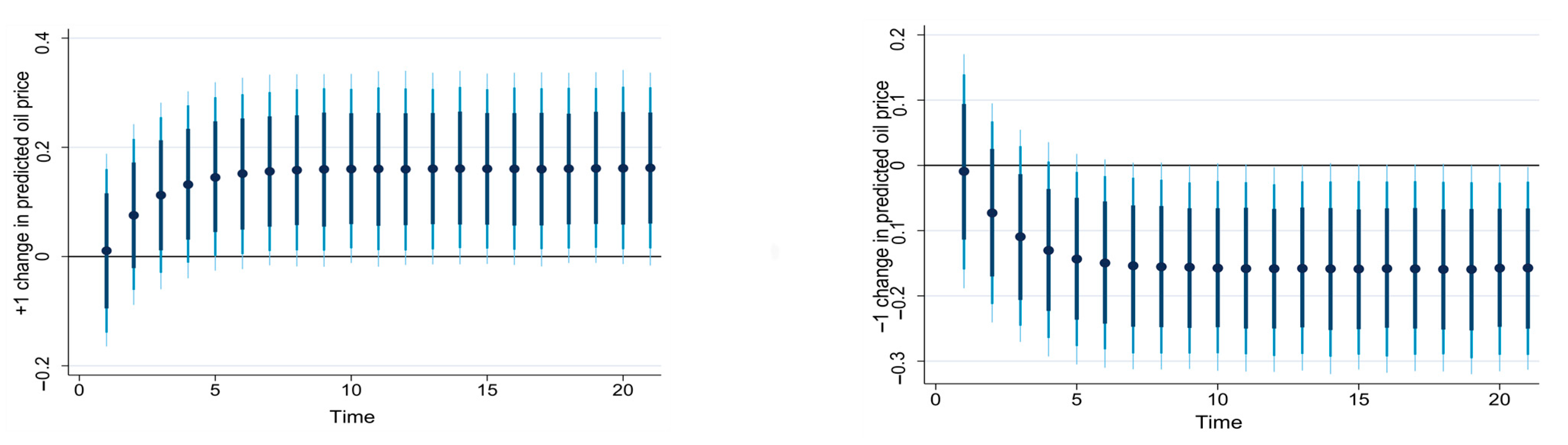
To better understand how renewable energy consumption responds to changes in fossil fuel prices, we used a new feature of the dynamic ARDL simulation model to predict, simulate, and plot the impact of a counterfactual change in the explanatory variable (fossil fuel prices) on the dependent variable (renewable energy consumption) while keeping other explanatory variables unchanged. In other words, the graphs allow plotting the impulse response of renewable energy consumption to fossil fuel prices in the short and long run. Figure 1 separately plots the response of renewable energy consumption to a ±1% change in predicted oil price, coal price, and natural gas price.

As shown, a 1% increase in oil prices has a long-run positive effect on renewable energy consumption. The short-run impact of oil increase is weak and not statistically significant. Starting from about t = 5, the impact of oil price increases is stabilized. Likewise, a 1% decline in oil prices negatively affects renewable energy only in the long run. Nevertheless, the same plot reveals the absence of significant short-run effects of oil price changes (increase and decrease). Figure 1 also shows that a 1% increase in coal price affects renewable energy use in the short- and long-run. However, the short-run effect is weak and increases to reach its maximum in the long run. The decline in coal price by 1% reduces the demand for renewable energy in the short and long run. Finally, the impact of natural gas price increases (decreases) is positive (negative) and results in a rise (decline) in renewable energy consumption in the long run. Another important remark that might emerge from Figure 1 is that the long-run impact of coal price upturns (decreases) is higher than that of oil prices and natural gas prices.

4.4. Dynamic ARDL Simulations with Structural Breaks

In this section, we check the validity of our prior findings when structural breaks are considered. To this end, a two-stage procedure was followed. First, we identified the dates of breakpoints in fossil fuel prices using the Bai–Perron multiple breakpoint test. Then, we re-used the dynamic ARDL simulations approach by introducing time dummies corresponding to breakpoints obtained from the Bai–Perron test. The results of the Bai–Perron multiple breakpoint test are reported in

Table 6. Results of Bai–Perron multiple breakpoint test.

	F-Statistic	Critical Values			Significant Breakpoint Dates
		1%	5%	10%
Oil price
$0 \mathrm{vs}. 1$	62.474 ***	12.290	8.580	7.040	2005
$1 \mathrm{vs}. 2$	40.492 ***	13.890	10.130	8.510	1986
$2 \mathrm{vs}. 3$	22.019 ***	14.800	11.140	9.410	1999
$3 \mathrm{vs}. 4$	9.425	15.280	11.830	10.040	NA
Coal price
$0 \mathrm{vs}. 1$	48.156 ***	12.290	8.580	7.040	2007
$1 \mathrm{vs}. 2$	22.973 ***	13.890	10.130	8.510	1986
$2 \mathrm{vs}. 3$	2.689	13.890	10.130	8.510	NA
Natural gas price
$0\mathrm{vs}.1$	38.403 ***	12.290	8.580	7.040	2000
$1\mathrm{vs}.2$	27.132 ***	13.890	10.130	8.510	1987
$2\mathrm{vs}.3$	20.989 ***	14.800	11.140	9.410	2014
$3\mathrm{vs}.4$	0.880	15.280	11.830	10.040	NA

Note: The maximum number of breakpoints was set to 5. The sequential testing of $l+1$ vs. $l$ breaks was used to detect the number and dates of significant breakpoints. *** denotes the rejection of the null hypothesis at 1% level.

. The maximum number of breakpoints was limited to five. The number and dates of significant breakpoints were endogenously determined based on the sequential testing of l + 1 vs. l breaks proposed by Bai and Perron [17,18]. The null hypothesis of l breakpoint was tested against the alternative of l + 1 breakpoint at year t.

As shown, the findings of the sequential test suggest rejecting the null of 0, 1, and 2 breakpoints in favor of the alternative of 1, 2, and 3 breakpoints for oil and natural gas prices, and rejecting the null of 0 and 1 breakpoints in favor of the alternative of 1 and 2 breakpoints for coal price. Therefore, the table suggests the presence of three significant breakpoints for oil price (2005, 1986, and 1999), two significant breakpoints for coal price (2007 and 1986), and three significant breakpoints for the natural gas price (2000, 1987, and 2014). The breakpoints mentioned above are significant at the 1% level for oil, coal, and natural gas prices.

We then introduced the endogenously determined breakpoint dates in models 1–3 and re-estimated them using the dynamic ARDL simulations. The results are reported in

Table 7. Results of the dynamically simulated ARDL with structural breaks model.

	$\mathit{M}\mathit{o}\mathit{d}\mathit{e}\mathit{l} 1$		$\mathit{M}\mathit{o}\mathit{d}\mathit{e}\mathit{l} 2$		$\mathit{M}\mathit{o}\mathit{d}\mathit{e}\mathit{l} 3$
	Coef.	p-Value	Coef.	p-Value	Coef.	p-Value
$Error correction term$	−0.518 ***	0.000	−0.436 ***	0.000	−0.369 ***	0.000
$paten{t}_{t-1}$	0.107 ***	0.008	0.105 **	0.013	0.098 ***	0.003
$\Delta patent$	0.034	0.421	0.058	0.168	−0.008	0.837
$gd{p}_{t-1}$	0.471 ***	0.003	0.386 **	0.016	0.233 *	0.065
$\Delta gdp$	−0.423	0.485	−0.189	0.601	−0.928 *	0.073
$carbo{n}_{t-1}$	0.039	0.804	0.074	0.682	0.236 *	0.092
$\Delta carbon$	−0.650	0.117	−0.189	0.601	−0.523	0.170
$fd{i}_{t-1}$	−4.190 ***	0.003	−3.574 ***	0.009	−3.725 ***	0.003
$\Delta fdi$	1.300	0.361	1.000	0.477	1.613	0.214
$oil{p}_{t-1}$	0.095 **	0.018	–	–	–	–
$\Delta oilp$	−0.002	0.965	–	–	–	–
$coal{p}_{t-1}$	–	–	0.121	0.105	–	–
$\Delta coalp$	–	–	0.105	0.139	–	–
$gas{p}_{t-1}$	–	–	–	–	0.085 **	0.034
$\Delta gasp$	–	–	–	–	−0.016	0.761
$d86$	0.098	0.318	0.085	0.374	–	–
$\Delta d86$	0.073	0.371	0.033	0.619	–	–
$d87$	–	–	–	–	0.067	0.415
$\Delta d87$	–	–	–	–	0.011	0.840
$d99$	−0.221 *	0.084
$\Delta d99$	−0.035	0.604
$d00$	–	–	–	–	0.0001	0.999
$\Delta d00$	–	–	–	–	−0.142 **	0.048
$d05$	−0.043	0.645	–	–	–	–
$\Delta d05$	0.005	0.925	–	–	–	–
$d07$	–	–	−0.013	0.908	–	–
$\Delta d07$	–	–	−0.042	0.535	–	–
$d14$	–	–	–	–	−0.042	0.594
$\Delta d14$	–	–	–	–	0.009	0.852
$constant$	7.506 *	0.069	6.249	0.148	9.880 ***	0.010
$Simulations$	10,000			10,000		10,000
$R^2$	0.747			0.696		0.813
$Prob.>F$	0.010			0.010		0.000

Note: ***, **, and * represent the statistical significance at 1%, 5%, and 10%, respectively.

. The table suggests the validity of previous results. Indeed, the long-run impact of oil prices on renewable energy use is positive and statistically significant at the 5% level, whereas no significant impact was identified in the short run. The findings also indicate that natural gas price positively and significantly affects renewable energy consumption in the long run with a coefficient of 0.085. Finally, the coefficient associated with coal price is also positive and weakly significant in the long run. However, the impacts of natural gas and coal prices are not statistically significant in the short run. Furthermore, the analysis suggests that following the introduction of time dummies, the long-run effects of oil prices and natural gas prices on renewable energy have been amplified and became more significant, while the magnitude and significance of the impact of coal prices fell. Finally, the error-correction terms associated with all models are significant at 1% and negative, confirming the long-run relationships between fossil fuel prices and renewable energy consumption. As in Table 6, patents on environmental technologies and gross domestic products positively affect renewable energy in the long run, while foreign direct investments are negatively associated with renewable energy.

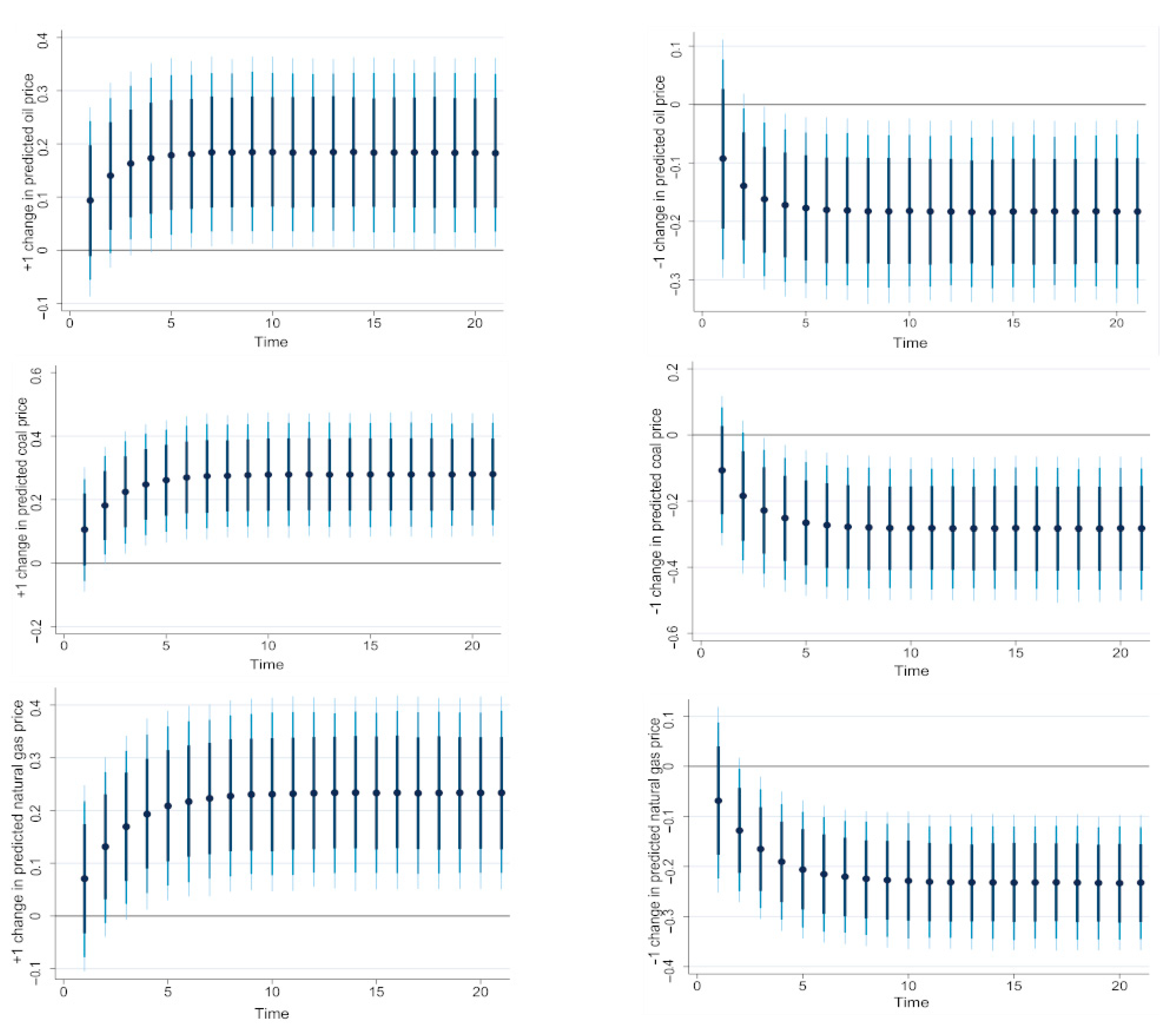
Overall, considering structural breaks did not affect the main results of the dynamic ARDL simulation procedure, which indicates that rising fossil fuel prices boost renewable energy consumption in the long run. To better detect the effects of fossil fuel prices on renewable energy consumption through the augmented dynamic ARDL simulation procedure, we plotted the prediction of changes of an explanatory variable and its outcome on the dependent variable, all else being equal. Figure 2 plots the response of renewable energy use to a 1% increase and decrease in oil, coal, and natural gas prices. The figure confirms the findings previously reached. Indeed, a 1% increase (decreases) in oil, coal, and natural gas prices positively (negatively) affects renewable energy only in the long run. These effects are not found to be significant in the short run.

5. Concluding Remarks

The past few decades have seen the rise of clean energy sources in all aspects of human life. A growing body of literature has been devoted to the key drivers of clean energy development. This study is part of the continuing debate about how to increase the share of clean energy sources in the energy mix. More precisely, we empirically investigated the effects of fossil fuel prices, specifically oil, coal, and natural gas, on renewable energy use in China from 1980 to 2018. To this end, the analysis was conducted based on the novel dynamic ARDL simulations procedure proposed by Philips [13] and Jordan and Philips [14], which has the advantage of predicting, stimulating, and plotting the impact of a counterfactual change in the explanatory variable on the dependent variable, all else being equal. Beyond fossil fuel prices, we incorporated gross domestic product, carbon dioxide emissions, environmental technologies patents, and foreign direct investments as control variables.

The initial data exploration using the bootstrap ADF and Lumsdaine and Papell’s [33] unit root tests suggests that all considered variables are integrated of order 0 or 1, and therefore, the suitability of the ARDL approach is verified. Moreover, we found strong evidence of long-run cointegrating relationship between the prices of all fossil fuels and renewable energy consumption. When estimating the short- and long-run effects using the dynamic ARDL simulations, the findings show that patents on environmental technologies and gross domestic product positively affect long-term renewable energy use. In contrast, foreign direct investments have adverse effects on renewables. Turning to fossil fuel prices, increasing oil, coal, and natural gas prices led to a rise in renewable energy in the long run. However, there is no evidence that oil, coal, and natural gas prices significantly affect renewable energy in the short run. These results confirm that renewable energy sources can eventually substitute fossil fuel energy in the long run. The impulse response plots confirm that both positive and negative shocks in oil, coal, and natural gas prices have long-run effects on renewable energy consumption. However, the highest impact is recorded for coal price. Finally, coal price also affects renewable energy consumption in the short run. When considering the presence of structural breaks, the results confirm the robustness of the dynamic ARDL simulations, as we conclude that fossil fuel prices affect renewable energy consumption only in the long run. Plots of the dynamic ARDL simulations with structural breaks show that the 1% increase (decrease) in oil, coal, and natural gas prices affects renewable energy consumption only in the long run. The short-run effects are not found to be statistically significant.

References

1. British Petroleum. BP Statistical Review of World Energy. June 2020. Available online: https://www.bp.com/en/global/corporate/energy-economics/statistical-review-of-world-energy.html (accessed on 15 June 2021).
2. Bayale, N.; Ali, E.; Tchagnao, A.F.; Nakumuryango, A. Determinants of renewable energy production in WAEMU countries: New empirical insights and policy implications. Int. J. Green Energy 2021, 18, 602–614. [Google Scholar] [CrossRef]
3. Akintande, O.J.; Olubusoye, O.E.; Adenikinju, A.F.; Olanrewaju, B.T. Modeling the determinants of renewable energy consumption: Evidence from the five most populous nations in Africa. Energy 2020, 206, 117992. [Google Scholar] [CrossRef]
4. Przychodzen, W.; Przychodzen, J. Determinants of renewable energy production in transition economies: A panel data approach. Energy 2020, 191, 116583. [Google Scholar] [CrossRef]
5. Murshed, M.; Tanha, M.M. Oil price shocks and renewable energy transition: Empirical evidence from net oil-importing South Asian economies. Energy Ecol. Environ. 2021, 6, 183–203. [Google Scholar] [CrossRef]
6. Zhao, Y.; Zhang, Y.; Wei, W. Quantifying international oil price shocks on renewable energy development in China. Appl. Econ. 2021, 53, 329–344. [Google Scholar] [CrossRef]
7. Brini, R.; Amara, M.; Jemmali, H. Renewable energy consumption, International trade, oil price and economic growth inter-linkages: The case of Tunisia. Renew. Sust. Energ. Rev. 2017, 76, 620–627. [Google Scholar] [CrossRef]
8. Apergis, N.; Payne, J.E. The causal dynamics between renewable energy, real GDP, emissions and oil prices: Evidence from OECD countries. Appl. Econ. 2014, 46, 4519–4525. [Google Scholar] [CrossRef]
9. Apergis, N.; Payne, J.E. Renewable energy, output, CO2 emissions, and fossil fuel prices in Central America: Evidence from a nonlinear panel smooth transition vector error correction model. Energ. Econ. 2014, 42, 226–232. [Google Scholar] [CrossRef]
10. Apergis, N.; Payne, J.E. Renewable energy, output, carbon dioxide emissions, and oil prices: Evidence from South America. Energ. Source. Part B 2015, 10, 281–287. [Google Scholar] [CrossRef]
11. Karacan, R.; Mukhtarov, S.; Barış, İ.; İşleyen, A.; Yardımcı, M.E. The Impact of Oil Price on Transition toward Renewable Energy Consumption? Evidence from Russia. Energies 2021, 14, 2947. [Google Scholar] [CrossRef]
12. Rhodium Group. China’s Greenhouse Gas Emissions Exceeded the Developed World for the First Time in 2019. Available online: https://rhg.com/research/chinas-emissions-surpass-developed-countries (accessed on 23 July 2021).
13. Philips, A.Q. Have your cake and eat it too? Cointegration and dynamic inference from autoregressive distributed lag models. Am. J. Polit. Sci. 2018, 62, 230–244. [Google Scholar] [CrossRef] [Green Version]
14. Jordan, S.; Philips, A.Q. Cointegration testing and dynamic simulations of autoregressive distributed lag models. Stata J. 2018, 18, 902–923. [Google Scholar] [CrossRef] [Green Version]
15. Abbasi, K.R.; Shahbaz, M.; Jiao, Z.; Tufail, M. How energy consumption, industrial growth, urbanization, and CO2 emissions affect economic growth in Pakistan? A novel dynamic ARDL simulations approach. Energy 2021, 221, 119793. [Google Scholar] [CrossRef]
16. Pesaran, M.H.; Shin, Y.; Smith, R.J. Bounds testing approaches to the analysis of level relationships. J. Appl. Econ. 2001, 16, 289–326. [Google Scholar] [CrossRef]
17. Bai, J.; Perron, P. Estimating and testing linear models with multiple structural changes. Econometrica 1998, 66, 47–78. [Google Scholar] [CrossRef]
18. Bai, J.; Perron, P. Computation and analysis of multiple structural change models. J. Appl. Econ. 2003, 18, 1–22. [Google Scholar] [CrossRef] [Green Version]
19. Büyüközkan, G.; Güleryüz, S. An integrated DEMATEL-ANP approach for renewable energy resources selection in Turkey. Int. J. Prod. Econ. 2016, 182, 435–448. [Google Scholar] [CrossRef]
20. Marques, A.C.; Fuinhas, J.A.; Manso, J.P. Motivations driving renewable energy in European countries: A panel data approach. Energ. Policy 2010, 38, 6877–6885. [Google Scholar] [CrossRef]
21. Aguirre, M.; Ibikunle, G. Determinants of renewable energy growth: A global sample analysis. Energ. Policy 2014, 69, 374–384. [Google Scholar] [CrossRef] [Green Version]
22. Damette, O.; Marques, A.C. Renewable energy drivers: A panel cointegration approach. Appl. Econ. 2019, 51, 2793–2806. [Google Scholar] [CrossRef]
23. Kumar, S.; Fujii, H.; Managi, S. Substitute or complement? Assessing renewable and nonrenewable energy in OECD countries. Appl. Econ. 2015, 47, 1438–1459. [Google Scholar] [CrossRef] [Green Version]
24. Gozgor, G.; Mahalik, M.K.; Demir, E.; Padhan, H. The impact of economic globalization on renewable energy in the OECD countries. Energ. Policy 2020, 139, 111365. [Google Scholar] [CrossRef]
25. Padhan, H.; Padhang, P.C.; Tiwari, A.K.; Ahmed, R.; Hammoudeh, S. Renewable energy consumption and robust globalization (s) in OECD countries: Do oil, carbon emissions and economic activity matter? Energy Strateg. Rev. 2020, 32, 100535. [Google Scholar] [CrossRef]
26. Bamati, N.; Raoofi, A. Development level and the impact of technological factor on renewable energy production. Renew. Energ. 2020, 151, 946–955. [Google Scholar] [CrossRef]
27. Guo, Y.; Yu, C.; Zhang, H.; Cheng, H. Asymmetric between oil prices and renewable energy consumption in the G7 countries. Energy 2021, 226, 120319. [Google Scholar]
28. Li, R.; Leung, G.C. The relationship between energy prices, economic growth and renewable energy consumption: Evidence from Europe. Energ. Rep. 2021, 7, 1712–1719. [Google Scholar]
29. Doytch, N.; Narayan, S. Does FDI influence renewable energy consumption? An analysis of sectoral FDI impact on renewable and non-renewable industrial energy consumption. Energ. Econ. 2016, 54, 291–301. [Google Scholar] [CrossRef]
30. Sam, C.Y.; McNown, R.; Goh, S.K. An augmented autoregressive distributed lag bounds test for cointegration. Econ. Model. 2019, 80, 130–141. [Google Scholar] [CrossRef]
31. Sarkodie, S.A.; Owusu, P.A. How to apply the novel dynamic ARDL simulations (dynardl) and Kernel-based regularized least squares (krls). MethodsX 2020, 7, 101160. [Google Scholar] [CrossRef]
32. Pata, U.K.; Caglar, A.E. Investigating the EKC hypothesis with renewable energy consumption, human capital, globalization and trade openness for China: Evidence from augmented ARDL approach with a structural break. Energy 2021, 216, 119220. [Google Scholar]
33. Lumsdaine, R.L.; Papell, D.H. Multiple trend breaks and the unit-root hypothesis. Rev. Econ. Stat. 1997, 79, 212–218. [Google Scholar] [CrossRef]
34. Kripfganz, S.; Schneider, D.C. Response surface regressions for critical value bounds and approximate p-values in equilibrium correction models. Oxford B Econ. Stat. 2020, 82, 1456–1481. [Google Scholar] [CrossRef]
35. Ben-Salha, O. Economic globalization, wages and wage inequality in Tunisia: An ARDL bounds testing approach. Rev. Middle East Econ. Financ. 2013, 9, 321–356. [Google Scholar] [CrossRef]
36. Akpan, U.F. Cointegration, Causality and Wagner’s Hypothesis: Time Series Evidence for Nigeria, 1970–2008. J. Econ. Res. 2011, 16, 59–84. [Google Scholar]
37. Sarkodie, S.A.; Strezov, V.; Weldekidan, H.; Asamoah, E.F.; Owusu, P.A.; Doyi, I.N.Y. Environmental sustainability assessment using dynamic autoregressive-distributed lag simulations—nexus between greenhouse gas emissions, biomass energy, food and economic growth. Sci. Total Environ. 2019, 668, 318–332. [Google Scholar] [CrossRef] [PubMed]
38. Dorta, M.; Sanchez, G. Bootstrap unit-root test for random walk with drift: The bsrwalkdrift command. Stata J. 2021, 21, 39–50. [Google Scholar] [CrossRef]
39. Westerlund, J.; Edgerton, D.L. A panel bootstrap cointegration test. Econ. Lett. 2007, 97, 185–190. [Google Scholar] [CrossRef]
40. Westerlund, J. Testing for error correction in panel data. Oxford B. Econ. Stat. 2007, 69, 709–748. [Google Scholar] [CrossRef] [Green Version]
41. Pedroni, P. Critical values for cointegration tests in heterogeneous panels with multiple regressors. Oxford B. Econ. Stat. 1999, 61, 653–670. [Google Scholar] [CrossRef]
42. Pedroni, P. Fully modified OLS for heterogeneous cointegrated panels. In Nonstationary Panels, Panel Cointegration, and Dynamic Panels (93–130); Baltagi, B.H., Fomby, T.B., Hill, R.C., Eds.; Emerald Group Publishing Limited: Bingley, UK, 2001. [Google Scholar]
43. Marinaș, M.C.; Dinu, M.; Socol, A.G.; Socol, C. Renewable energy consumption and economic growth. Causality relationship in Central and Eastern European countries. PLoS ONE 2018, 13, e0202951. [Google Scholar] [CrossRef] [Green Version]
44. Radmehr, R.; Henneberry, S.R.; Shayanmehr, S. Renewable energy consumption, CO2 emissions, and economic growth nexus: A simultaneity spatial modeling analysis of EU countries. Struct. Chang. Econ. Dynamic 2021, 57, 13–27. [Google Scholar] [CrossRef]
45. Zhao, P.; Lu, Z.; Fang, J.; Paramati, S.R.; Jiang, K. Determinants of renewable and non-renewable energy demand in China. Struct. Change. Econ. D 2020, 54, 202–209. [Google Scholar] [CrossRef]
46. Jun, W.; Zakaria, M.; Shahzad, S.J.H.; Mahmood, H. Effect of FDI on pollution in China: New insights based on wavelet approach. Sustainability 2018, 10, 3859. [Google Scholar] [CrossRef] [Green Version]
47. Cheng, Z.; Li, L.; Liu, J. The impact of foreign direct investment on urban PM2.5 pollution in China. J. Environ. Manag. 2020, 265, 110532. [Google Scholar] [CrossRef] [PubMed]
48. Lu, X.; Zhang, S.; Xing, J.; Wang, Y.; Chen, W.; Ding, D.; Wu, Y.; Wang, X.; Duan, L.; Hao, J. Progress of air pollution control in China and its challenges and opportunities in the ecological civilization era. Engineering 2020, 6, 1423–1431. [Google Scholar] [CrossRef]
49. Wang, Z.; Yang, Z.; Zhang, Y.; Yin, J. Energy technology patents–CO2 emissions nexus: An empirical analysis from China. Energ. Policy 2012, 42, 248–260. [Google Scholar] [CrossRef]
Figure 1. Representation of (±1%) counterfactual shocks in predicted oil, coal, and natural gas prices on renewable energy consumption using dynamic ARDL simulations. Dots show the mean change in predicted value from sample mean, while the shaded lines (from darkest to lightest) represent the 75%, 90%, and 95% confidence intervals.
Sustainability 14 10439 g001aSustainability 14 10439 g001b
Figure 2. Representation of (±1%) counterfactual shocks in predicted oil, coal, and natural gas prices on renewable energy consumption using dynamic ARDL simulations with structural breaks. Dots show the mean change in predicted value from sample mean, while the shaded lines (from darkest to lightest) represent the 75%, 90%, and 95% confidence intervals.
Sustainability 14 10439 g002