Article

Space–Time Effect of Green Total Factor Productivity in Mineral Resources Industry in China: Based on Space–Time Semivariogram and SPVAR Model

1
School of Economics, Yunnan University of Finance and Economics, Kunming 650221, China
2
School of Urban and Environment, Yunnan University of Finance and Economics, Kunming 650221, China
3
Yunnan Land Resources Planning and Design Research Institute, Kunming 650216, China
*
Author to whom correspondence should be addressed.
Sustainability 2022, 14(14), 8956; https://doi.org/10.3390/su14148956
Submission received: 9 June 2022 / Revised: 14 July 2022 / Accepted: 20 July 2022 / Published: 21 July 2022
(This article belongs to the Special Issue Advances in Manufacturing Sustainability in the Industry 4.0 Era)

Abstract

:
Improving green total factor productivity (GTFP) is the key for China’s mineral resources industry to get out of the dilemma of resource depletion and environmental degradation. The Super Slacks-Based Measure (Super-SBM) model with undesirable output is used to calculate the GTFP of China’s mineral resources industry between 2004 and 2019, and the space–time correlation threshold is quantitatively determined by the space–time semivariogram. On this basis, the spatial weight matrix is constructed, and the spatial panel vector autoregression (SPVAR) model is used to quantitatively estimate the space–time impact response among GTFP, import dependence, and R&D investment. The results show that: (1) The maximum range of mineral resources industry GTFP in time and space are 12.28 years and 635.28 km, respectively. Taking the space range as the correlation distance threshold to construct spatial weight matrix improves the accuracy of spatial analysis. (2) The increase in import dependence and R&D investment can effectively improve the GTFP of local and its neighboring provinces. In the long term, an increase in import dependence has a positive impact on R&D investment, and an increase in R&D investment can reduce the import dependence. (3) In the response to impact, the eastern region is greater than the western region, the coastal provinces are greater than the inland provinces, and the provinces close to the impact source are greater than the provinces far away. Therefore, policies to limit resource and energy consumption, pollution, and carbon emissions should be strengthened. The incentive policies should be emphasized differently and adopted for the impact sources and response areas. The R&D investment in the full mineral industry process should be increased to improve the GTFP.

1. Introduction

The mineral resources industry provides basic material resources for mankind and supports the prosperity and development of the world economy and society. China is a major producer and consumer of global mineral resources and has an important influence on the world’s mineral resources industry market. In the long term, China’s demand of mineral resources will remain at a high level. The rapid development of the mineral resources industry has led to excessive resource consumption, serious carbon emissions, and low resource utilization efficiency [1]. According to the China Industrial Statistical Yearbook and Carbon Emission Accounts and Datasets’ (CEADs) data, the operating revenue of China’s mineral resources industry (including mining, smelting, and processing industries) accounted for 25.28%, energy consumption accounted for 43.27%, and carbon emissions accounted for 33.87% of the industry in 2019. Undoubtedly, the mineral resources industry is a high energy consumption and high emission industry. The resource and environmental problems caused by this extensive development patten threaten the future sustainable development of China’s mineral resources industry. Under the context of a low-carbon economy, more and more countries are paying attention to reducing resource and energy consumption and carbon emissions. The mineral resources industry is constantly transitioning to one that is green, safe, and efficient. Improving green total factor productivity (GTFP) has become the only way for China’s mineral resources industry to get out of the dilemma of resource depletion and environmental degradation.
At present, the research hotspots on GTFP of industries are mainly focused on the following aspects:
(1) Definition of the concept and measurement framework. Total factor productivity (TFP) measures the efficiency of converting all inputs into final outputs [2,3], and it is mainly used in the study of economic growth and sustainable development. In the early research on TFP, only the capital element input and economic benefits of output were considered [4,5]. With the deepening of research, scholars have found that resource consumption and environmental pollution are issues that cannot be ignored in sustainable development and should be included in the analysis framework, then GTFP emerges as the times require [6,7]. Considering the importance of the mineral resources industry in the development of the global economy and the disturbance to the resource environment during the mining and production process of mineral resources, the GTFP of the mineral resources industry has attracted more and more attention of scholars in recent years [8,9,10]. Resource and environmental indicators such as fossil fuels, energy consumption, carbon emissions, waste gas, waste-water, and solid wastes have been continuously incorporated into the analysis framework of the mineral resources industry GTFP [11,12,13], which has improved the accuracy of the measurement of sustainable development of the mineral resources industry.
(2) GTFP is influenced by many factors, and the perspective of research is constantly changing from non-spatial to spatial effects. A large number of studies have shown that factors such as industrial agglomeration [14,15] and environmental regulation [16] have impacts on regional or industrial TFP. Due to the extremely uneven spatial distribution of mineral resources in the world, the global trade of mineral products is frequent, and import and export become an important factor affecting GTFP [17]. It is found that import not only has a unidirectional influence on TFP, but also an interactive relationship among TFP, imports, and R&D investment. Import is accompanied by technology inflow, which is conducive to improving the overall level of R&D [18]; moreover, import and R&D are conducive to competition, stimulating innovation and learning, and promoting the improvement of TFP [19,20,21]. Through in-depth study, scholars found that TFP and importation have obvious spatial correlation. These relationships not only exist locally, but also bring spatial spillover effects to surrounding areas. Import, combined with local and surrounding R&D, will bring sustained and stable growth of TFP [22,23,24]. However, as an indispensable aspect of the sustainable development of China’s mineral resources industry, there are few achievements in the exploration of the interaction relationship and spatial effects of the three variables.
(3) In terms of research methods, a spatial model has become a research hotspot in recent years. The spatial relationships of regional economies are measured by the spatial weight matrix. Building a more reasonable spatial weight matrix can improve the accuracy of spatial effect analysis. The commonly used spatial weight matrix mainly includes a single matrix such as adjacency relationship, geographical distance, and economic distance, or a composite spatial weight matrix such as economic geography [25,26,27]. Geographic distance can be widely used to measure the influence from far to near. In practical applications, in order to improve the estimation effect, spatial association needs to be limited within a certain range, and a geographic distance threshold is usually set. The distance threshold of spatial weight matrix can be determined directly according to the scale of the research object [28] by using the inflection point of the U-shaped influence relationship as the threshold [16], or by using continuous regression to improve the accuracy [29].
At present, most studies on GTFP focus on industry and region, while there are fewer studies on GTFP in mineral resources industry, literature on the space–time effects of GTFP in mineral resources industry from the perspective of international trade is extremely rare. Although factors such as energy and environment have been included in the GTFP measurement in the mineral resources industry, the consideration of resource inputs is not comprehensive enough. With the deepening of spatial analysis, a large number of scholars have used spatial econometric models to determine whether variables have impacts on GTFP; however, few studies have focused on the affect process. This paper focuses on how imports and R&D affect GTFP from a spatial perspective. The spatial weight matrix is the key parameter to reflect spatial relationships, while its objective determination is difficult. This paper tries to improve the accuracy of spatial weight matrix construction by quantitatively measuring the spatial relevance distance as a threshold with the space–time semivariogram. Through the accurate measurement and space–time evolution analysis of GTFP in the mineral resources industry, as well as the simulation of the space–time impact response of import and R&D investment to GTFP, the results can provide a scientific basis for the sustainable development of mineral resources industry in China, and also provide a more accurate basis for the formulation of policies related to spatial layout, import, and R&D investment of the mineral resources industry.
The contributions of this paper can be summarized in three points. Resource inputs are incorporated into the GTFP analysis framework of mineral resources industry to improve the accuracy of measurement. An attempt to combine the space–time semivariogram with the SPVAR model improves the accuracy of the spatial effect analysis. The SPVAR model is used to analyze the response process of the mineral resources industry GTFP that is impacted by import and R&D investment in space.

2. Materials and Methods
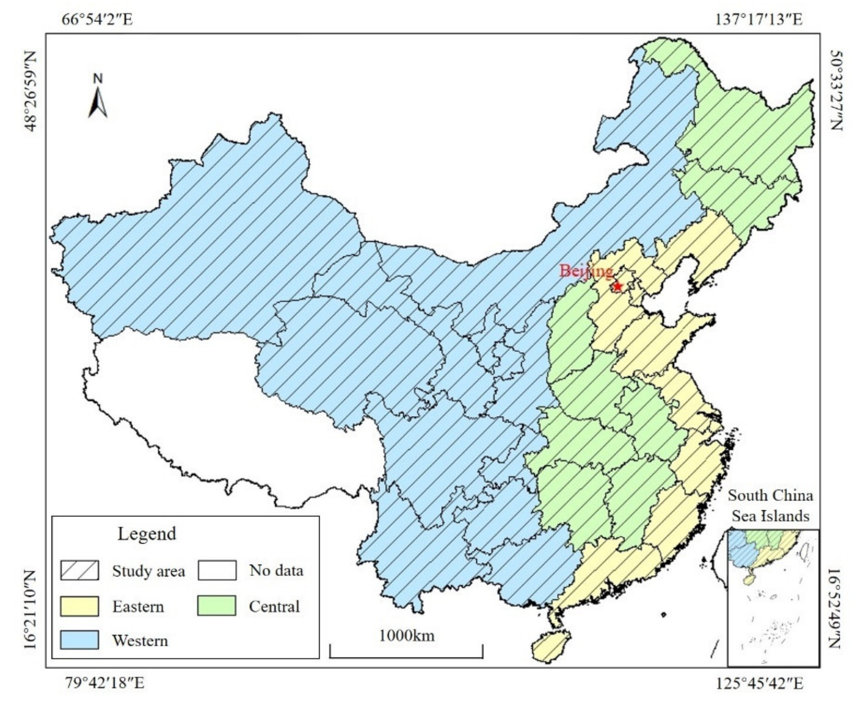
2.1. Study Area

The study area includes data from 30 provinces in China (excluding Tibet, Hong Kong, Macao, and Taiwan). The spatial location of each province is represented by the coordinates of the provincial capital city. The calculation range of space–time semivariogram is set as rectangle, as shown in Figure 1.

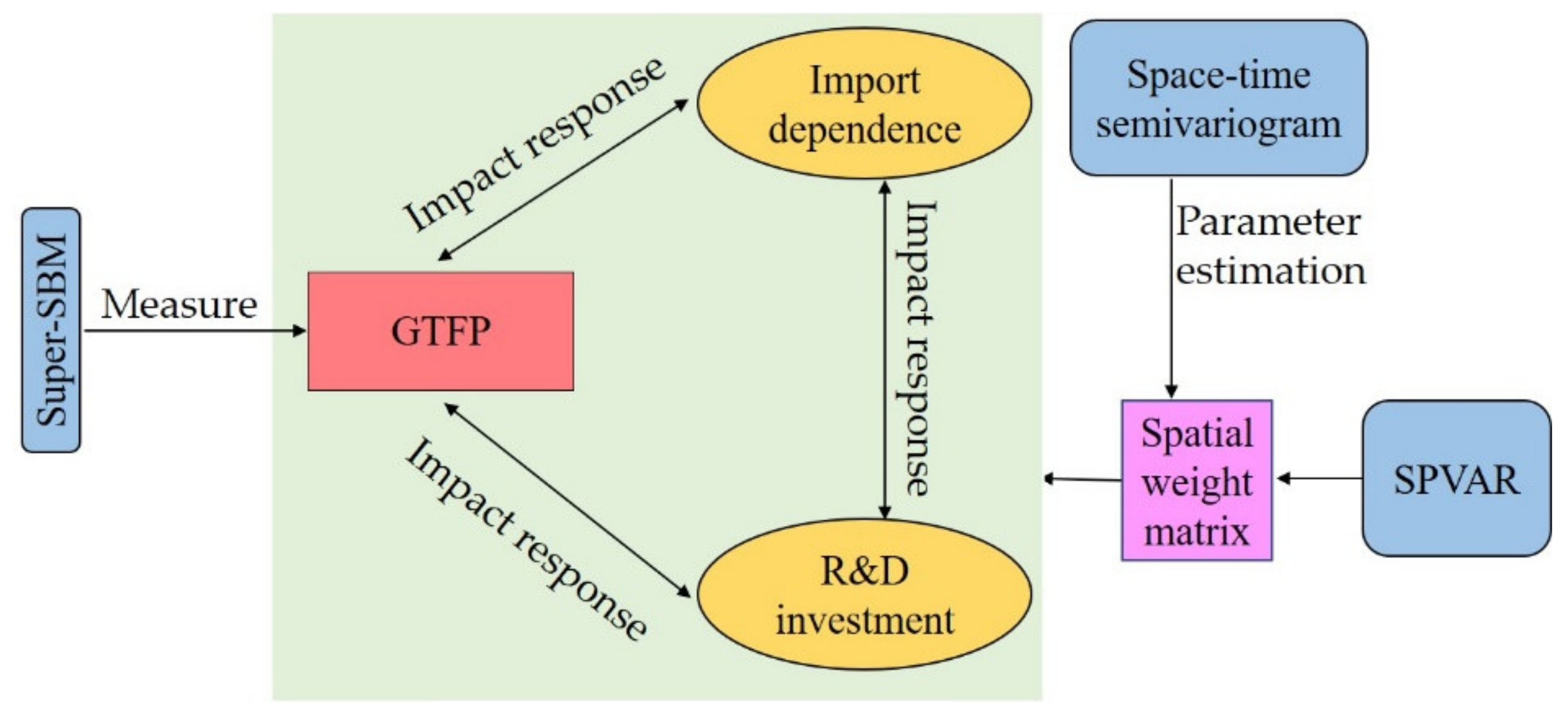
2.2. Methodological Analysis Framework

The research contents mainly include GTFP measurement of mineral resources industry and the space–time impact response analysis among GTFP, import dependence, and R&D investment. The main research method is the SPVAR model, which is used to explore the space–time impact response (Figure 2). The Super-SBM model is used to measure GTFP of mineral resources industry, and space–time semivariogram is used to construct the spatial weight matrix, which is the key parameter in SPVAR.

2.3. Super Slacks-Based Measure (SBM) Model

Compared with the radial efficiency measurement of CCR and BCC models, the Slacks-Based Measure model (SBM) can avoid overestimating the actual efficiency, measure the excess inputs and insufficient outputs, and decompose and measure the efficiency of each element by relaxation. In order to further consider the undesirable outputs and overcome the problem that the effective decision-making unit (DMU) cannot be compared when the efficiency is greater than 1 [30,31], the Super-SBM model, including undesirable output, is used for measurement, and its calculation formula is:
ϕ * = min 1 m i = 1 m x ¯ i x i 0 1 s 1 + s 2 r = 1 s 1 y ¯ r 1 g y r 10 g + u = 1 s 2 y ¯ r 2 b y r 20 b s . t . x ¯ j = 1 , 0 n λ j x j , j = 1 , , m y ¯ g j = 1 , 0 n λ j y j g , r = 1 , , s 1 y ¯ b j = 1 , 0 n λ j y j b , l = 1 , , s 2 x ¯ x 0 , y ¯ s y 0 s , y ¯ b y 0 b , λ 0 , j = 1 , 0 n λ j = 1
where, ϕ * is the efficiency. x is the input. y g is the desirable output. y b is the undesirable output. λ is a non-negative multiplier vector for linear programming. “-” above the variable represents the projected value. The larger the value of ϕ * , the higher the efficiency level. When ϕ * is greater than or equal to 1, it means that all slack variables are 0 s 0 = 0 , s 0 g = 0 , s 0 b = 0 .

2.4. Space–Time Semivariogram

The GTFP of the mineral resources industry shows the characteristics of correlation and randomness in time and space. It is difficult to describe the complete space–time semivariogram of the GTFP in the mineral resources industry with only a single deterministic or purely stochastic model. The space–time semivariogram can not only represent the continuity of changes, but also show the randomness of changes. It is an effective analysis method to describe the space–time variability of GTFP in mineral resources industry.
Space–time semivariogram is extended from the traditional variogram [32,33].
Let Z u ; u R d + 1 be a multivariate space–time random field which has the following form of matrix equation:
u = s , t , s = s s , s 2 , , s d D R d   ( generally   d = 3 )  
t T R is the temporal coordinate, and D × T R d + 1 is the spatial coordinate.
If the space–time variable Z u satisfies the second-order stationary, then its expectation, M , is independent of u = s , t , while the space–time variables Z u and Z u + h depend on the space–time separation vector, h = h s , h t . Where h s and h t represent the interval in space domain and time domain, respectively.
In order to model the experimental space–time semivariogram, two models can be used: the integrated product model and the integrated product–sum model. It is generally considered that the integrated product–sum model is better than the integrated product model [34,35,36]. Another model of space–time semivariogram is polynomial expression for nested structures [37]. The space–time semivariogram model γ s t h s , h t is expressed directly by the sum of a series of functions, f i , with the coefficient, τ i :
γ s t h s , h t = i τ i f i h s , h t
In practicality, the polynomial expression holds the same characteristics as the sum of different types of elementary semivariograms. In order to improve the polynomial form of the space–time semivariogram, tensor product cubic smoothing surface can be used. The tensor product function, S h s , h t , is the product of two basic independent functions f h s and g h t , and is multiplied by the weighting coefficient b k l .
S h s , h t = k = 0 K l = 0 L b k l f k h s g l h t  
where K and L are the orders of f and g , respectively. In the case of a cubic spline function, K and L are 3, with 16 unknown b k l . Considering that the first and second derivatives of S must be continuous at all the lags h s , h t , 15 independent conditions are needed to determine the function. In addition, it is necessary to balance the two criteria between (1) the closeness of the function to the experimental semivariogram data and (2) its smoothness, as defined by small curvature. Generally, the balance weight of all h s , h t can be equal.

2.5. Spatial Panel VAR (SPVAR)

Spatial econometric technology introduces spatial effect into traditional econometric methods, which can reflect the influence of spatial factors. The spatial panel vector autoregression model (SPVAR) is an endogenous system that includes both temporal and spatial factors. It can be used for the study of multivariable space–time interaction [38,39]. The vector autoregression model with spatial elements can significantly reduce the prediction error.
The three variables of GTFP, import dependence (IMD), and R&D investment (RD) of the mineral resources industry interact in time and space. Considering the synchronous influence, time lag influence, and spatial lag influence among variables, a SPVAR model is constructed to analyze the “impact-response” process among the three variables. In order to simplify the analysis, the SPVAR model with a time lag 1 order and space lag 1 order is shown as follows:
G T F P i t = β 11 I M D i t + β 12 R D i t + θ 11 I M D i , t 1 + θ 12 G T F P i , t 1 + θ 13 R D i , t 1 + γ 11 I M D ˜ i , t 1 + γ 12 G T F P ˜ i , t 1 + γ 13 R D ˜ i , t 1 + μ 1 t I M D i t = β 21 G T F P i t + β 22 R D i t + θ 21 I M D i , t 1 + θ 22 G T F P i , t 1 + θ 23 R D i , t 1 + γ 21 I M D ˜ i , t 1 + γ 22 G T F P ˜ i , t 1 + γ 23 R D ˜ i , t 1 + μ 2 t R D i t = β 31 I M D i t + β 32 G T F P i t + θ 31 I M D i , t 1 + θ 32 G T F P i , t 1 + θ 33 R D i , t 1 + γ 31 I M D ˜ i , t 1 + γ 32 G T F P ˜ i , t 1 + γ 33 R D ˜ i , t 1 + μ 3 t
where GTFP, IMD and RD are explanatory variables. β i j , θ i j , and γ i j are the coefficients. y ˜ i , t 1 = i = 1 n w i j y i , t 1 is the 1 order cross term of space–time lag in the endogenous variable. w i j is the spatial weight coefficient. i is the province. t is the time. μ is the random disturbance term.
The spatial weight coefficient adopts the geographic distance spatial weight matrix W = w i j . Among them, the threshold of the correlation distance is measured objectively and quantitatively by the range fitted by space–time semivariogram. The formula is as follows:
w i j = 1 / d i j 2 0 d i j a   and   i j 0 d i j > a   or   i = j
where w i j is the element in row i and column j of the spatial weight matrix. d i j is the straight-line distance from the capital of i province to the capital of j province. a is the range of the GTFP of the mineral resources industry. Beyond the range, it is considered that the relationship between the two provinces can be ignored, and the weight element is set to 0.

2.6. Sample Selection and Data Sources

The sample data of mineral resources industry ranges from 2004 to 2019.

2.6.1. Selection of Input and Output Indicators

GTFP measures the overall efficiency of transforming all inputs into the final output, in which resource and energy consumption and environmental pollution need to be included in the analysis framework. In addition to considering the desirable output, the measurement of the GTFP of the mineral resources industry also needs to consider the undesirable output and reflect the resource input, so as to more comprehensively reflect the relationship between the production efficiency and the cost of resources and environment of mineral resources industry. In previous studies, although fossil fuels and energy consumption have been contained in the input indicators as resource inputs, these indicators cannot fully represent the input of mineral resources.
This paper selects resource input, energy input, capital input, and labor input as input indicators of GTFP of mineral resources, mineral sales output value as desirable output, and CO2 emissions as undesirable output. Due to the more comprehensive consideration of the resource input, the GTFP of the mineral resources industry measured in this paper is more accurate.
The resource input is represented by the total output value of the raw ore industry. In order to unify the differences in the type, quantity, and value of the resource input, the total output value of the raw ore industry in the China Mining Yearbook is used and deflated according to the ex-factory price index.
Energy input is represented in energy consumption. The energy consumption of the mineral resources industry in the “CEADs Database” is used for summary calculation and converted into standard coal. Among them, the input of oil, natural gas, and coal is calculated in the resource input, and this part of the input is excluded when calculating the energy input.
Capital input is represented by capital stock. The fixed asset investment data is used in “China fixed asset investment database”. According to the provincial fixed asset investment price index (2004 as the base period), the deflator is processed, and the perpetual inventory method is used for accounting [40].
Labor input is represented by the number of employed persons at the end of the year. The number of employed persons in the mineral resources industry of each province is measured by using the “China Industrial Economic Database”.
Desirable output is represented by the sales output value. The sales output value data of mineral resources industry is used in the “China Industrial Economic Database”. Taking 2004 as the base period, the industrial producer price index of each province is used for deflator processing.
Undesirable output is represented by CO2 emission. The CO2 emission of the mineral resources industry is used in the “CEADs database”.

2.6.2. Data Sources of Space–Time Semivariogram Indicators

The calculation data of space–time semivariogram adopts the GTFP of the mineral resources industry, including 30 provinces in China from 2004 to 2019, with a total of 30 × 16 = 480 annual data.

2.6.3. Data Sources of SPVAR Model Indicators

The SPVAR model adopts the data of GTFP, IMD, and RD of mineral resources industry.
GTFP adopts the calculation results of the Super-SBM model with undesirable output.
IMD is expressed as a percentage of imports to the total output value. The data on the import value of the mineral resources industry comes from the “Guoyan Network” in China.
RD is calculated according to the R&D investment and operating income data of listed companies in the mineral resources industry from the “Guotai’an” database in China.
The interpolation method is used to estimate the missing data for the above variables.

3. Results

3.1. Measurement Result of GTFP

Using the Super-SBM model with an undesirable output, the mean of the GTFP of the mineral resources industry in 30 provinces in China from 2004 to 2019 was calculated (Table 1). The mean of the GTFP of the mineral resources industry in the 30 provinces is 0.424. The largest province is Hainan (0.958), and the smallest province is Heilongjiang (0.141). Most of the provinces have a low level of GTFP in the mineral resources industry. From the calculation results, resource input as an independent variable suggests that the GTFP and the annual growth rate are not so overestimated [41,42].
The following will further analyze the change law of GTFP in each province in time and space.

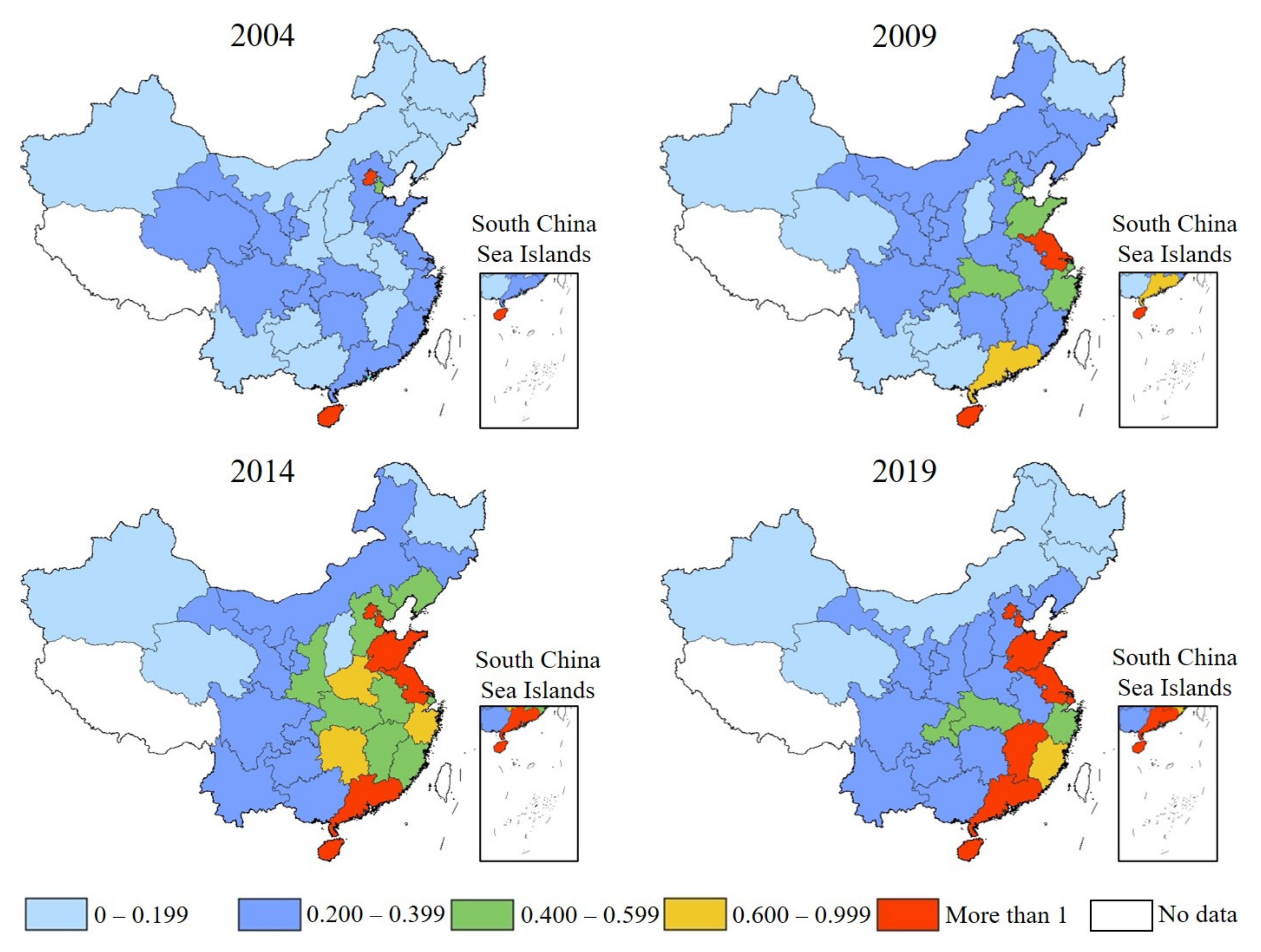
3.2. Space–Time Evolution Analysis of GTFP

There are obvious regional differences in the spatial distribution of GTFP in the mineral resources industry. In order to analyze its space–time evolution law, it is necessary to group the data. The GTFP of the mineral resources industry is generally low. In the results calculated by the Super-SBM model, the high-efficiency provinces have an efficiency value greater than 1. According to the distribution characteristics of GTFP, the grouping standard is determined and divided into five groups (Figure 3).
From the spatial distribution map, it can be seen that the spatial distribution of GTFP in each province has obvious spatial correlation, and that the spatial interdependence between provinces is obvious.
The GTFP has increased significantly in the time trend, which is mainly due to the improvement of the comprehensive utilization efficiency of resources and energy and the improvement of the pollution control level in the production process. From the perspective of spatial trends, high-efficiency provinces continue to gather in coastal areas, which effectively drives the improvement of GTFP in neighboring provinces. Due to the convenience of sea and land transportation, coastal provinces are the main sources and processing places for the import of mineral products, saving transportation and economic costs. They have become the high-value distribution areas of GTFP. This is consistent with the existing research results on the distribution of GTFP in China’s mineral resources industry [41,43].

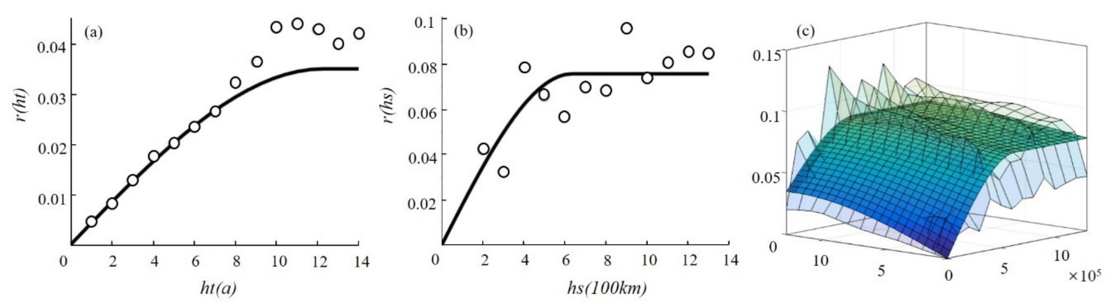
3.3. Space-Time Semivariogram Analysis of GTFP

According to the distribution characteristics of GTFP in time and space, the parameters for calculating the space–time semivariogram are determined.
The GTFP data are annual data, the total timespan is 16 years, and the distribution is regular. Therefore, when calculating the space–time semivariogram, the time step (interval), error, and number are set as 1 year, 0.5 years, and 14 years, respectively.
The GTFP data are geodetic coordinate data in space. The maximum separation distance of GTFP is 3492 km, the minimum separation distance is 122 km, and the most of separation distances are about 1400 km. The spatial distribution of coordinates is irregular. When calculating the space–time semivariogram, the spatial step (interval), error, and number are set as 100 km, 50 km, and 12 km, respectively.
According to the distribution of the calculated results of the experimental time boundary semivariogram (Figure 4a) and the experimental space boundary semivariogram (Figure 4b), the spherical model is selected to fit the theoretical time and space boundary semivariogram. Furthermore, the integrated product–sum model and the tensor product cubic smoothing surface model can be used to fit the theoretical model of the space–time semivariogram. The experimental space–time semivariogram and the theoretical space–time semivariogram can be presented in the same figure (Figure 4c).
The spatial range of the space–time semivariogram of the GTFP of mineral resources industry is 635.28 km, the sill value is 0, and the arch height is 0.076, which has a strong spatial correlation in the range of 635.28 km. The time range is 12.28 years, the sill value is 0, and the arch height value is 0.035, which has a strong time correlation in the range of 12.28 years.
The fitting degree of the time boundary semivariogram is better than that of the space boundary semivariogram; its range is larger, and its arch height is more obvious, indicating that the GTFP of mineral resources has a greater correlation in time and has better continuity and correlation, while the spatial continuity and correlation are relatively small.
Overall, the space–time semivariogram can quantitatively measure the spatial semivariogram and temporal semivariogram distance of the GTFP of the mineral resources industry.
Using the results calculated by space–time, the spatial weight matrix in SPVAR is calculated. The capital Urumqi of Xinjiang province is about 1462 km away from the capital Xining of Qinghai province and 1621 km away from the capital Lanzhou of Gansu province, both exceeding the range of 635.28 km. If the geographical distance is 0, Xinjiang has no neighboring province, therefore the distance between the two provinces is retained.
Compared with the traditional method of determining the threshold in the spatial weight matrix [29], using the space–time semivariogram to calculate the spatial range as the threshold can more accurately reflect the objective reality.

3.4. Space–Time Impact Response

Before using the SPVAR model, firstly, the stationarity test of variables is carried out. Secondly, the Granger causality test is carried out to analyze whether there is an interactive relationship between variables. Third, the spatial correlation of all variables is tested.
The data of GTFP, IMD, and RD in the mineral resources industry from 2004 to 2019 are used for a series of tests. The stationarity test results show that the three variables have significant stationarity. The Granger causality test shows that there is a pairwise Granger causality relationship among the three variables. The spatial correlation test shows that GTFP and IMD have a significant positive spatial correlation in each year, while RD has a significant spatial correlation in 9 out of 16 years. Therefore, the SPVAR model can be used for parameter estimation of the three variables.

3.4.1. Estimation Results

It can be found from the model estimation results (Table 2) that the coefficients of the time lag term and the space–time lag cross term are significant, indicating that it is reasonable to add spatial factors to the model. Adding space–time lag cross term can obtain a more ideal forecast. However, the endogenous variable system of the model will cause the interpretation of the parameter estimation results to have no practical significance [44]. It is necessary to further simulate the space–time impact response generated by the mutual impact of the three variables.

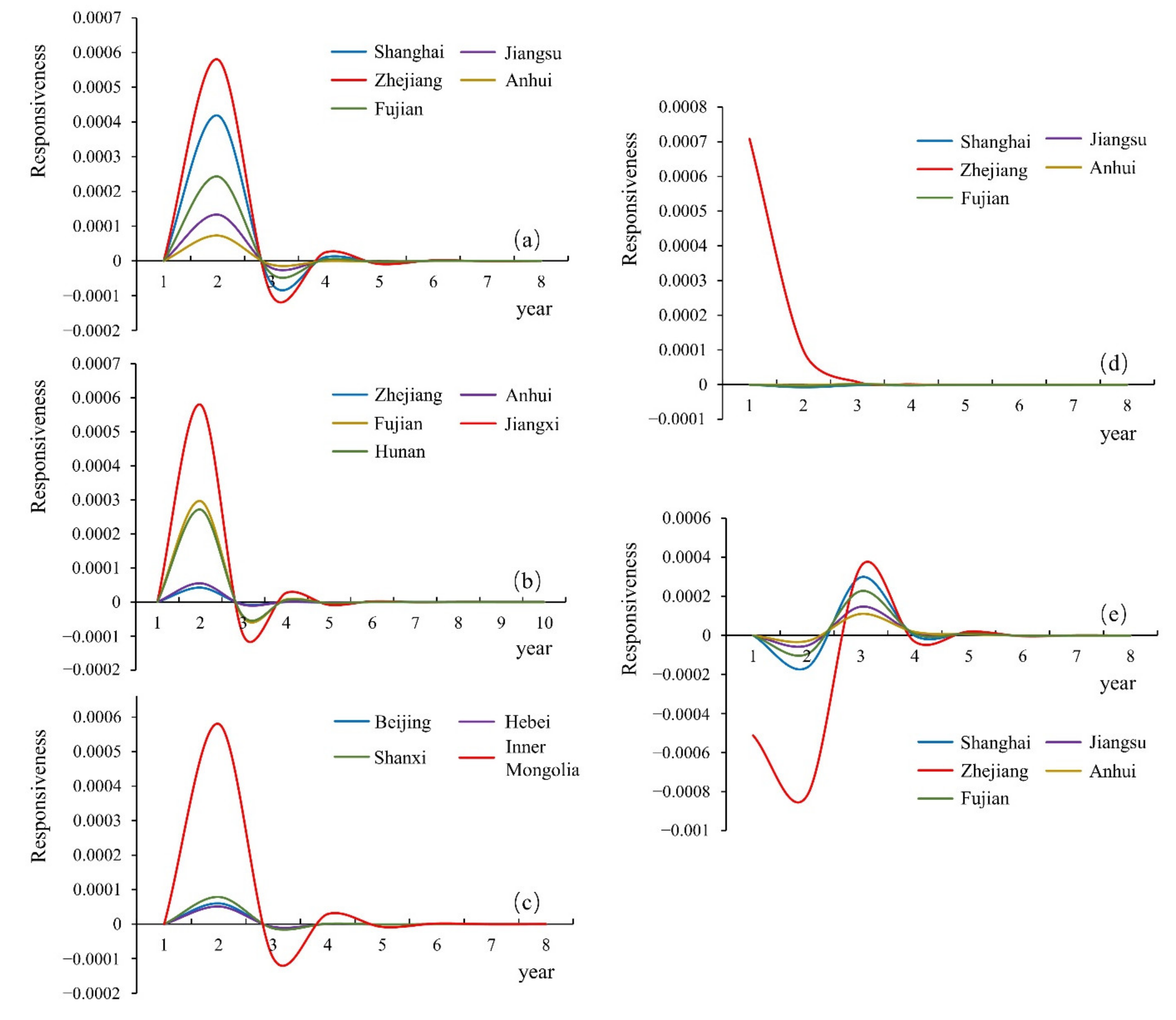
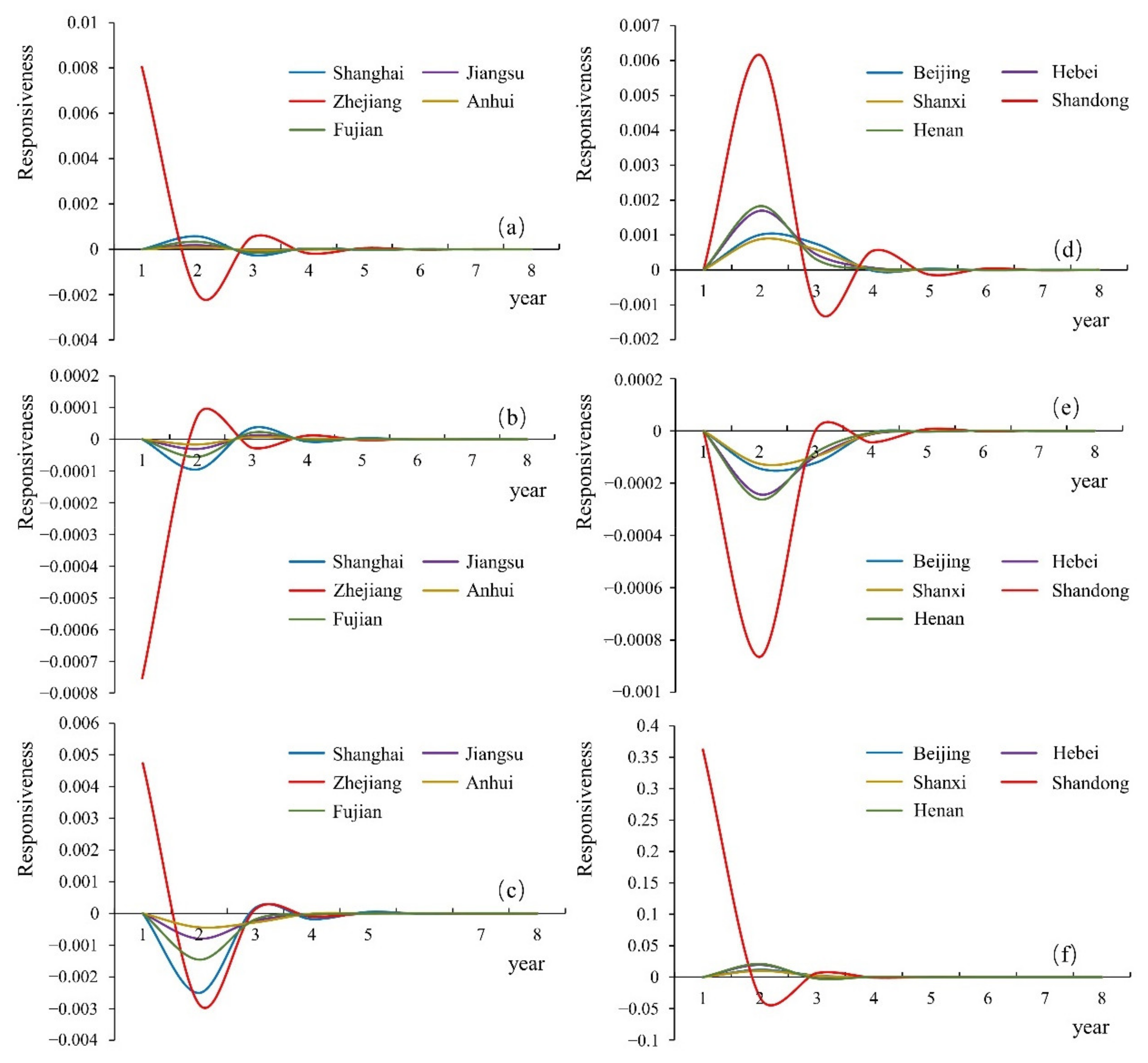
3.4.2. Impact Response Analysis

The impact source of the impact response of the SPVAR model can be various variables, and the response can be reflected in time and space. The impact from a province will gradually spread to the surrounding provinces over time, and the response degree and way will vary in different regions, which can be expressed through the spatial weight matrix.
For the 30 regions and 3 variables, n × k 2 = 30 × 3 2 = 270 ( n is 30 regions and k is 3 endogenous variables), and impact response graphs can be generated. For demonstrating the main points, this paper selects several representative provinces as the impact source to analyze the impact process to the adjacent provinces.
1.
IMD as impact source
In order to analyze the impact response process of IMD as an impact source to GTFP, Zhejiang, Jiangxi, and Inner Mongolia were selected as representative impact sources in the eastern, central, and western regions to analyze the impact response process to neighboring provinces.
According to the distance from near to far, there are four selected neighboring provinces of Zhejiang, namely Shanghai, Jiangsu, Anhui, and Fujian, used to analyze the impact response process. Moreover, four neighboring provinces of Jiangxi are selected, namely Hunan, Anhui, Fujian, and Zhejiang. In the same way, there are three neighboring provinces of Inner Mongolia, namely Shanxi, Beijing, and Hebei.
From the simulation results (Figure 5), under the positive impact of one standard deviation from IMD, the three variables all presented space–time responses of different ranges and directions in the local and neighboring provinces.
Under the positive impact of one standard deviation of IMD from Zhejiang province, the response of the GTFP in the local and neighboring provinces is obviously positive in two years. The maximum local response occurred in the second year, and the response ranges of the neighboring provinces varied. Jiangxi and Inner Mongolia had the same situation as Zhejiang province. The GTFP response on neighboring provinces shows three characteristics: (1) the neighboring provinces are affected the most in the eastern region, somewhat in the central region, and the least in the western region. (2) Due to more convenient shipping and higher import dependence, the coastal provinces are more affected than the inland provinces. (3) The closer the province is to the impact source, the greater the response. The reason is that imported ores can reduce resource input costs and carbon emissions, and the inflow of technology accompanying imports can also improve production efficiency, which also improves GTFP.
Under the positive impact of one standard deviation of IMD from Zhejiang province, the response of IMD is obviously positive in the local province; however, it is very weak in the neighboring provinces. This coincides with the actual situation of mineral resources. The import channels of the mineral resources of each province are generally fixed.
Under the positive impact of one standard deviation of IMD from Zhejiang Province, the response of RD in the local and neighboring provinces will first be negative, then be positive, and, finally, tends to be stable within two years. The inflow of technology accompanying mineral products’ import will have a certain “crowding out” effect on local RD in the short term due to factors such as secrets, technology protection, and competition. However, in the medium and long term, mineral products import will promote local RD. After a certain period of technical learning and knowledge innovation, GTFP can be effectively improved.
2.
GTFP as impact sources
With relatively higher GTFP, the Zhejiang province is selected as the representative impact source. According to the distance from near to far, there are four selected provinces, namely Shanghai, Jiangsu, Anhui, and Fujian, taken to analyze the impact response process.
Under the positive impact of one standard deviation of GTFP from Zhejiang province, the three variables in the local and neighboring provinces all produced space–time responses (Figure 6a–c). The response intensity of coastal provinces is higher than inland provinces, and near regions are higher than far regions.
Under the positive impact of one standard deviation of the GTFP from Zhejiang province, the response of the local GTFP is strongly positive in the first year, then alternates between negative and positive, and the response degree continues to decrease to stability. The response of the GTFP in neighboring provinces is slightly positive.
Under the positive impact of one standard deviation of the GTFP from the Zhejiang province, the response of IMD in local and neighboring provinces is negative, and then becomes positive. In the initial stage, due to the local mineral reserves and domestic supply, the improvement of GTFP will not decrease the IMD. However, along with the continuous expansion of demand, it is necessary to cover the shortage through importing minerals, resulting in an increase in import dependence. The improvement of GTFP will produce technology spillovers in neighboring provinces, therefore the demand for minerals in neighboring provinces will be relatively reduced, and the IMD will also decrease.
Under the positive impact of one standard deviation of the GTFP from the Zhejiang province, the response of local RD is positive in the first year and turned negative in the second year, while the response of RD in neighboring provinces was negative. Since the improvement of GTFP is mainly due to technological progress, the improvement of GTFP in the Zhejiang province will promote the local RD in the short term. Along with the continuous technology overflow from Zhejiang provinces, neighboring provinces can reduce RD by accepting technology transfer.
3.
RD as impact sources
With relatively high RD, Shandong Province is selected as the representative RD impact source region to analyze the impact response process to neighboring provinces. From near to far, four provinces, Hebei, Henan, Beijing, and Shanxi, adjacent to Shandong Province, were selected for analysis.
Under the positive impact of one standard deviation of RD from Shandong Province, the three variables all have different responses (Figure 6d–f). The overall response intensity shows that the provinces closer to Shandong are higher.
Under the positive impact of one standard deviation of RD from Shandong Province, the response of GTFP in local and neighboring provinces is positive. It shows that RD is conducive to improving GTFP. With the increase in RD, the technical level of mineral resources industry, the efficiency of resource utilization, and carbon emissions have been significantly improved, and local GTFP has also been effectively improved and has promoted the GTFP in surrounding areas.
Under the positive impact of one standard deviation of RD from Shandong Province, the response of IMD in local and neighboring provinces is negative. The RD can improve the resource utilization efficiency and can effectively reduce the import volume under the same demand.
Under the positive impact of one standard deviation of RD from Shandong Province, the response of local RD is significantly positive, while the response of neighboring provinces is weakly positive. The RD level in each province is relatively fixed. Although RD somewhat increases over time, it is more affected by the decisions of local enterprises and local governments, and is not affected by neighboring provinces.
Similar to the results found from a study on the TFP of Chinese industry or region [20,21], it also can be found that IMD and RD all have positive effects on GTFP. Using SPVAR, we can analyze the impact response process more clearly and accurately.

4. Discussion

Although there has been a lot of research on the GTFP of the mineral resources industry, there are still two points to be improved.
The first is related to the input of mineral resources. Most studies consider resource input by measuring GTFP, but do not fully incorporate it into the research framework. Usually, energy input is used as the only resource input variable. As the depletion of mineral resources becomes increasingly prominent, energy cannot fully represent mineral resources, and some scholars propose to use resource and energy as an input factor [45]. Due to the difficulty in obtaining and unifying the data of mineral resources, although resource input is proposed, t many quantitative measurements have been completed.
The second is the measurement method of GTFP spatial association. The spatial correlation of spatial units is measured by a spatial weight matrix. In some studies, the thresholds for the spatial correlation were determined using subjective empirical judgments or multiple regression tests [29,46]. This is reasonable to a certain extent; however, it is not rigorous enough. In contrast, taking the ranges of the space–time semivariogram as threshold improves the accuracy.
Therefore, this study attempts to make breakthroughs in the above two aspects. First, mineral resource input is fully considered. The gross industrial output value of raw ore is used to represent the resource input and is completely measured. The second is the space–time semivariation, which is used to calculate the spatial range of GTFP, which is used as the threshold of the spatial weight matrix for impact response analysis to improve the accuracy of the space–time effect analysis.

5. Conclusions

In this paper, the space–time semivariogram is used to calculate the threshold of the spatial correlation distance of GTFP, which is used to construct the spatial weight matrix of the SPVAR model to analyze the space–time impact responses among GTFP, IMD, and RD in the mineral resources industry. It is worth mentioning that resource input as an independent variable is introduced in the GTFP measurement, which improves the comprehensiveness and accuracy of GTFP for the mineral resources industry. The main conclusions include:
(1)
The space–time semivariation is used to calculate the space–time variability of the GTFP of the mineral resources industry. The maximum correlation distances of time and space are 12.28 years and 635.28 km, respectively. This is used as the threshold of the spatial weight matrix in space–time impact response analysis, which improves the accuracy of spatial analysis;
(2)
The impact response results among IMD, RD, and GTFP is as follows: IMD has an obvious positive effect on GTFP in local and neighboring provinces. The impact from IMD to RD in local and surrounding provinces first shows as negative and then turns to positive. GTFP has obvious negative effects on IMD in the local and neighboring provinces, and then turns to positive. GTFP, at first, has positive effects on local RD, and then turns to negative, while RD in neighboring provinces mainly shows as negative. The RD has obvious positive effects on GTFP in local and neighboring provinces. RD has a certain negative effect on IMD in local and neighboring provinces;
(3)
The neighboring provinces’ response degree is large in the eastern region, medium in the central region, and small in the western region. The coastal provinces’ response is greater than that in inland provinces. The neighboring provinces that are closer to the impact source have a greater response.
According to the above conclusions, to improve the GTFP in mineral resource industry could, by increasing the import on high quality mineral products, increase R&D investment to improve the technical level, strengthening different regulations in various regions to limit resource and environment input.
The study also suggests several avenues for future research. Firstly, although the selection of the input–output factors of the mineral resources industry in this paper is more comprehensive, it can still only represent the real GTFP to a certain extent. Secondly, the space–time semivariogram is used to calculate the time and spatial range of the GTFP of the mineral resources industry. However, in order to simplify the model and facilitate analysis, the spatial range is used in the construction of the SPVAR model with reference to the time range. In the next step, the accurate time lag term can be added to the model to improve the accuracy of model analysis.

Author Contributions

Investigation, Formal analysis, R.J.; Methodology, C.L.; Data Curation, X.L.; Writing—original draft preparation, R.J. and C.L.; Writing—review and editing, S.Z. All authors have read and agreed to the published version of the manuscript.

Funding

This research was supported by the National Natural Science Foundation of China (NSFC) [Grant No. 42062020].

Acknowledgments

Sincere thanks are extended to the anonymous reviewers and editors for their valuable comments and suggestions that helped improve the clarity of the manuscript.

Conflicts of Interest

The authors declare no conflict of interest.

References

  1. Mohsin, M.; Zhu, Q.; Naseem, S.; Sarfraz, M.; Ivascu, L. Mining industry impact on environmental sustainability, economic growth, social interaction, and public health: An application of semi-quantitative mathematical approach. Processes 2021, 9, 972. [Google Scholar] [CrossRef]
  2. Miao, J.; Wang, P. Bubbles and total factor productivity. Am. Econ. Rev. 2012, 102, 82–87. [Google Scholar] [CrossRef] [Green Version]
  3. Faluk, S.; Sun, S.; Hafiz, W.K.; Muhammed, S.H.; Muhammad, A.N.; Van, C.N. Assessing the efficiency and total factor productivity growth of the banking industry: Do environmental concerns matters? Environ. Sci. Pollut. Res. 2021, 28, 20822–20838. [Google Scholar]
  4. Coelli, T.J.; Rao, D. Total factor productivity growth in agriculture: A Malmquist index analysis of 93 countries, 1980–2000. Agric. Econ. 2005, 32, 115–134. [Google Scholar] [CrossRef] [Green Version]
  5. Chen, P.C.; Yu, M.M.; Chang, C.C.; Hsu, S.H. Total factor productivity growth in China’s agricultural sector. China Econ. Rev. 2008, 19, 580–593. [Google Scholar] [CrossRef]
  6. Chen, S.; Golley, J. ‘Green’ productivity growth in China’s industrial economy. Energy Econ. 2014, 44, 89–98. [Google Scholar] [CrossRef]
  7. Chen, C.; Lan, Q.; Ming, G.; Sun, Y. Green total factor productivity growth and its determinants in China’s industrial economy. Sustainability 2018, 10, 1052. [Google Scholar] [CrossRef] [Green Version]
  8. Zobrist, J.; Giger, W. Mining and the Environment. Environ. Sci. Pollut. Res. 2013, 20, 7487–7489. [Google Scholar] [CrossRef] [Green Version]
  9. Valderrama, C.V.; Santibaňez-González, E.; Pimentel, B.; Candia-Véjar, A.; Canales-Bustos, L. Designing an environmental supply chain network in the mining industry to reduce carbon emissions. J. Clean. Prod. 2020, 254, 119688. [Google Scholar] [CrossRef]
  10. Cheng, Z.; Li, L.; Liu, J. Natural resource abundance, resource industry dependence and economic green growth in China. Resour. Policy 2020, 68, 101734. [Google Scholar] [CrossRef]
  11. Feng, H.; Zhang, Q.; Lei, J.; Fu, W.; Xu, X. Energy efficiency and productivity change of China’s iron and steel industry: Accounting for undesirable outputs. Energy Policy 2013, 54, 204–213. [Google Scholar]
  12. Yu, Y.; Chen, Z.; Wei, L.; Wang, B. The low-carbon technology characteristics of China’s ferrous metal industry. J. Clean. Prod. 2017, 140, 1739–1748. [Google Scholar] [CrossRef]
  13. Zhu, X.; Chen, Y.; Feng, C. Green total factor productivity of China’s mining and quarrying industry: A global data envelopment analysis. Resour. Policy 2018, 57, 1–9. [Google Scholar] [CrossRef]
  14. Chen, W.; Huang, X.; Liu, Y.; Luan, X.; Song, Y. The impact of high-tech industry agglomeration on green economy efficiency—Evidence from the Yangtze river economic belt. Sustainability 2019, 11, 5189. [Google Scholar] [CrossRef] [Green Version]
  15. Wei, W.; Zhang, W.L.; Wen, J.; Wang, J.S.; Hall, S.; Pauly, P. TFP growth in Chinese cities: The role of factor-intensity and industrial agglomeration. Econ. Model. 2020, 91, 534–549. [Google Scholar] [CrossRef]
  16. Hu, W.; Wang, D. How does environmental regulation influence China’s carbon productivity? An empirical analysis based on the spatial spillover effect. J. Clean. Prod. 2020, 257, 120484. [Google Scholar] [CrossRef]
  17. Li, K.W.; Wang, T. Is Oil as a Financial Resource Productive? Available online: https://ssrn.com/abstract=3616526 (accessed on 30 May 2019).
  18. Mo, J.; Qiu, L.D.; Zhang, H.; Dong, X. What you import matters for productivity growth: Experience from Chinese manufacturing firms. J. Dev. Econ. 2021, 152, 102677. [Google Scholar] [CrossRef]
  19. Higon, D.A.; Manez, J.A.; Sanchis-Llopis, J.A. Intramural and external R&D: Evidence for complementarity or substitutability. Econ. Politica 2018, 35, 555–577. [Google Scholar]
  20. Ding, L.; Wu, M.; Jiao, Z.; Nie, Y. The positive role of trade openness in industrial green total factor productivity—Provincial evidence from China. Environ. Sci. Pollut. Res. 2021, 29, 6538–6551. [Google Scholar] [CrossRef]
  21. Huang, J.; Cai, X.; Huang, S.; Tian, S. Technological factors and total factor productivity in China: Evidence based on a panel threshold model—ScienceDirect. China Econ. Rev. 2019, 54, 271–285. [Google Scholar] [CrossRef]
  22. Audretsch, D.B.; Belitski, M. The role of R&D and knowledge spillovers in innovation and productivity. Eur. Econ. Rev. 2020, 123, 103391. [Google Scholar]
  23. Bengoa, M.; Román, V.M.S.; Pérez, P. Do R&D activities matter for productivity? A regional spatial approach assessing the role of human and social capital. Econ. Model. 2017, 160, 448–461. [Google Scholar]
  24. Liang, X.; Li, P. Empirical study of the spatial spillover effect of transportation infrastructure on green total factor productivity. Sustainability 2020, 13, 326. [Google Scholar] [CrossRef]
  25. Qu, X.; Lee, L. Estimating a spatial autoregressive model with an endogenous spatial weight matrix. J. Econom. 2015, 184, 209–232. [Google Scholar] [CrossRef]
  26. Guo, Y.Q.; Sun, X.F.; He, Y. Research on the incentive, growth performance and adjustment orientation of local fiscal leverage. Econ. Res. J. 2017, 52, 169–182. (In Chinese) [Google Scholar]
  27. Lam, C.; Souza, P.C.L. Estimation and selection of spatial weight matrix in a spatial lag model. J. Bus. Econ. Stat. 2020, 38, 693–710. [Google Scholar] [CrossRef]
  28. Fang, Z.; Razzaq, A.; Mohsin, M.; Irfan, M. Spatial spillovers and threshold effects of internet development and entrepreneurship on green innovation efficiency in China. Technol. Soc. 2022, 68, 101844. [Google Scholar] [CrossRef]
  29. Gong, W.; Ni, P.; Xu, H. The spatial spillover effect and spillover bandwidth of influential factors to urban economic competitiveness: Based on the spatial econometric analysis of 285 cities in China. Nanjing J. Soc. Sci. 2019, 9, 23–30, 38. (In Chinese) [Google Scholar]
  30. Tone, K. A slacks-based measure of super-efficiency in data envelopment analysis. Eur. J. Oper. Res. 2002, 143, 32–41. [Google Scholar] [CrossRef] [Green Version]
  31. Zhang, N.; Choi, Y. Environmental energy efficiency of China’s Regional Economies: A Non-oriented slacks-based measure approach. Soc. Sci. J. 2013, 50, 225–234. [Google Scholar] [CrossRef]
  32. Rouhani, S.; Wackernagel, H. Multivariate geostatistical approach to space-time data analysis. Water Resour. Res. 1990, 36, 585–591. [Google Scholar] [CrossRef] [Green Version]
  33. Goovaerts, P.; Sonnet, P. Study of Spatial and Temporal Variations of Hydrogeochemical Variables Using Factorial Kriging Analysis. In Geostatistics Troia’92; Springer: Dordrecht, The Netherlands, 1993; Volume 2, pp. 745–756. [Google Scholar]
  34. De Iaco, S.; Myers, D.E.; Posa, D. Space-time variograms and a functional form for total air pollution measurements. Comput. Stat. Data Anal. 2002, 41, 311–328. [Google Scholar] [CrossRef]
  35. Cressie, N.; Huang, H. Classes of nonseparable, spatial-temporal stationary covariance functions. J. Am. Stat. Assoc. 1999, 94, 1330–1340. [Google Scholar] [CrossRef]
  36. De Cesare, L.; Myers, D.E.; Posa, D. Estimating and modeling space-time correlation structures. Stat. Probab. Lett. 2001, 51, 9–14. [Google Scholar] [CrossRef]
  37. Liu, C.; Koike, K. Extending Multivariate Space-Time Geostatistics for Environmental Data Analysis. Math. Geosci. 2007, 39, 289–305. [Google Scholar] [CrossRef]
  38. Beenstock, M.; Felsenstein, D. Spatial vector autoregressions. Spat. Econ. Anal. 2007, 2, 167–196. [Google Scholar] [CrossRef] [Green Version]
  39. Márquez, M.A.; Ramajo, J.; Hewings, G.J.D. Regional growth and spatial spillovers: Evidence from an SpVAR for the Spanish regions. Pap. Reg. Sci. 2015, 94, S1–S18. [Google Scholar] [CrossRef]
  40. Zhang, J.; Wu, G.; Zhang, J. The Estimation of China’s provincial capital stock: 1952–2000. Econ. Res. J. 2004, 10, 35–44. (In Chinese) [Google Scholar]
  41. Feng, C.; Huang, J.B.; Wang, M. Analysis of green total-factor productivity in China’s regional metal industry: A meta-frontier approach. Resour. Policy 2018, 58, 219–229. [Google Scholar] [CrossRef]
  42. Ren, Y.J.; Wang, C.X.; Qi, Y.X.; Liang, D. An empirical study on the impact of resource-based industrial agglomeration on green total factor productivity. Stat. Decis. 2020, 36, 124–127. (In Chinese) [Google Scholar]
  43. Fang, C.; Cheng, J.; Zhu, Y.; Zhu, Y.; Chen, J.; Peng, X. Green Total Factor Productivity of Extractive Industries in China: An explanation from Technology Heterogeneity. Resour. Policy 2020, 70, 101933. [Google Scholar] [CrossRef]
  44. Kuethe, T.H.; Pede, V.O. Regional Housing Price Cycles: A Spatio-temporal Analysis Using US State-level Data. Reg. Stud. 2011, 45, 563–574. [Google Scholar] [CrossRef] [Green Version]
  45. Wang, X.; Sun, C.; Wang, S.; Zhang, Z.; Zou, W. Going green or going away? A spatial empirical examination of the relationship between environmental regulations, biased technological progress, and green total factor productivity. Int. J. Environ. Res. Public Health 2018, 15, 1917. [Google Scholar] [CrossRef] [Green Version]
  46. Huang, Y.; Yang, H. Identifying IFDI and OFDI productivity spatial spillovers: Evidence from China. Emerg. Mark. Financ. Trade 2020, 56, 1124–1145. [Google Scholar] [CrossRef]
Figure 1. Study area.
Sustainability 14 08956 g001
Figure 2. Methodological analysis framework of space–time impact response among GTFP, import dependence, and R&D investment in mineral resources industry.
Sustainability 14 08956 g002
Figure 3. Space–time evolution of GTFP in mineral resources industry.
Sustainability 14 08956 g003
Figure 4. Space–time semivariogram of the GTFP of mineral resources industry. (a) time boundary semivariogram; (b) space boundary semivariogram; (c) space–time semivariogram.
Sustainability 14 08956 g004
Figure 5. Space–time response of the IMD of the mineral resources industry as impact source: (a) impact of Zhejiang IMD on GTFP; (b) impact of Jiangxi IMD on GTFP; (c) impact of Inner Mongolia IMD on GTFP; (d) the impact of Zhejiang IMD on IMD; (e) impact of Zhejiang IMD on RD.
Sustainability 14 08956 g005
Figure 6. Space–time response of GTFP and RD of the mineral resources industry as impact source. (a) Impact of Zhejiang GTFP on GTFP; (b) impact of Zhejiang GTFP on IMD; (c) impact of Zhejiang GTFP on RD; (d) the impact of Shandong RD on GTFP; (e) impact of Shandong RD on IMD; (f) impact of Shandong RD on RD.
Sustainability 14 08956 g006
Table 1. Mean of GTFP of mineral resources industry from 2004 to 2019.
ProvinceGTFPProvinceGTFPProvinceGTFPProvinceGTFP
Beijing0.893Shanghai0.576Hubei0.426Yunnan0.213
Tianjin0.740Jiangsu0.871Hunan0.425Shaanxi0.322
Hebei0.374Zhejiang0.588Guangdong0.767Gansu0.298
Shanxi0.195Anhui0.292Guangxi0.216Qinghai0.201
Inner Mongolia0.211Fujian0.417Hainan0.958Ningxia0.305
Liaoning0.28Jiangxi0.524Chongqing0.374Xinjiang0.153
Jilin0.254Shandong0.711Sichuan0.329mean0.424
Heilongjiang0.141Henan0.479Guizhou0.204--
Table 2. Estimation results of SPVAR model parameters.
VariableGTFPIMDRD
GTFP (−1)0.33 * (0.19)−0.807 ** (0.40)0.017 * (0.01)
IMD (−1)0.023 * (0.01)0.136 (0.24)−0.002 (0.01)
RD (−1)0.418 (0.68)−1.223 (1.43)0.088 * (0.05)
W × GTFP (−1)0.01 (0.27)−0.95 ** (0.48)−0.032 * (0.02)
W × IMD (−1)0.019 (0.16)−0.021 (0.41)−0.005 (0.03)
W × RD (−1)0.739 * (0.44)−0.116 (2.42)0.368 ** (0.18)
Note: The data corresponding to each variable are parameter estimates, and the data in parentheses are standard errors. ** and * indicate significance at the statistical level of 5% and 10%, respectively. GTFP (−1), IMD (−1) and RD (−1) represent the time lag 1 order of GTFP, IMD and RD respectively. W × GTFP (−1), W × IMD (−1) and W × RD (−1) represent the 1 order cross term of the time-space lag of GTFP, IMD and RD respectively.
Publisher’s Note: MDPI stays neutral with regard to jurisdictional claims in published maps and institutional affiliations.

