
Spatially Explicit River Basin Models for Cost-Benefit Analyses to Optimize Land Use


Abstract
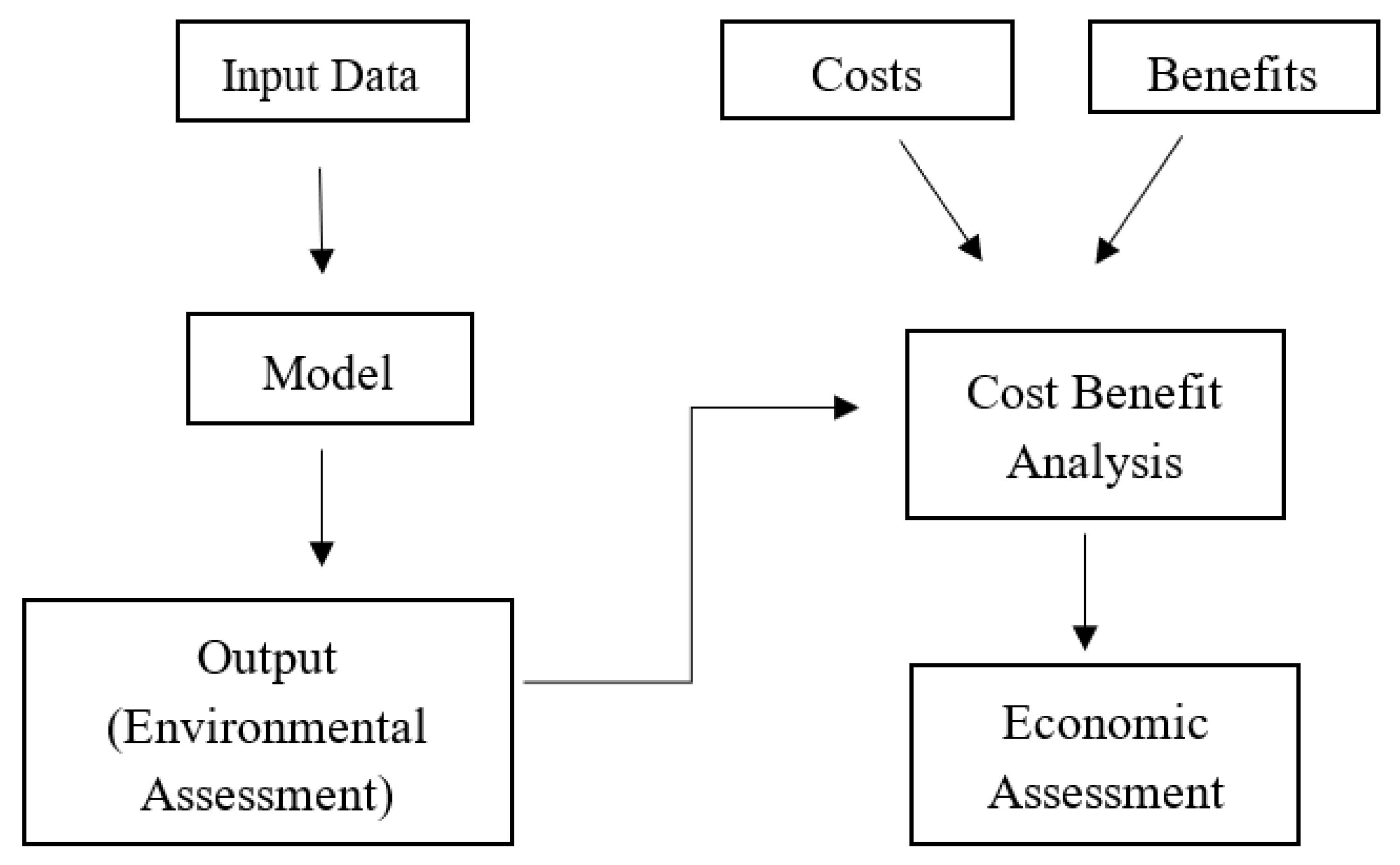
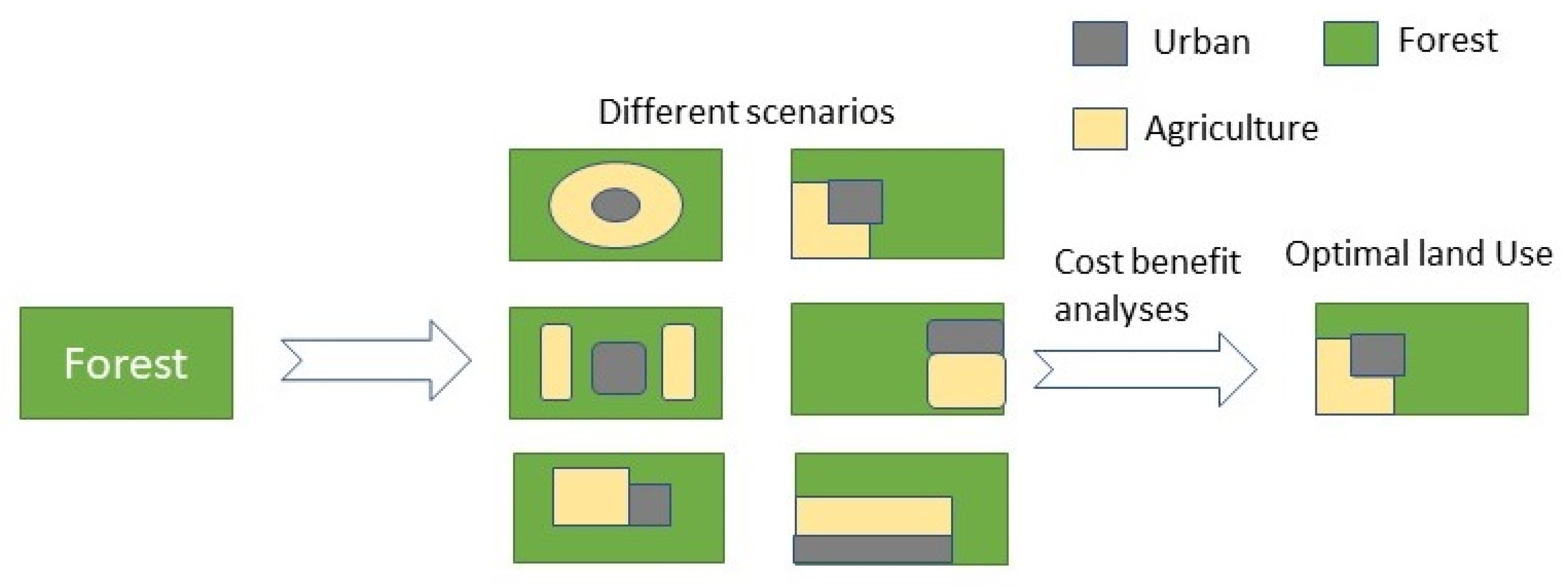
:1. Introduction
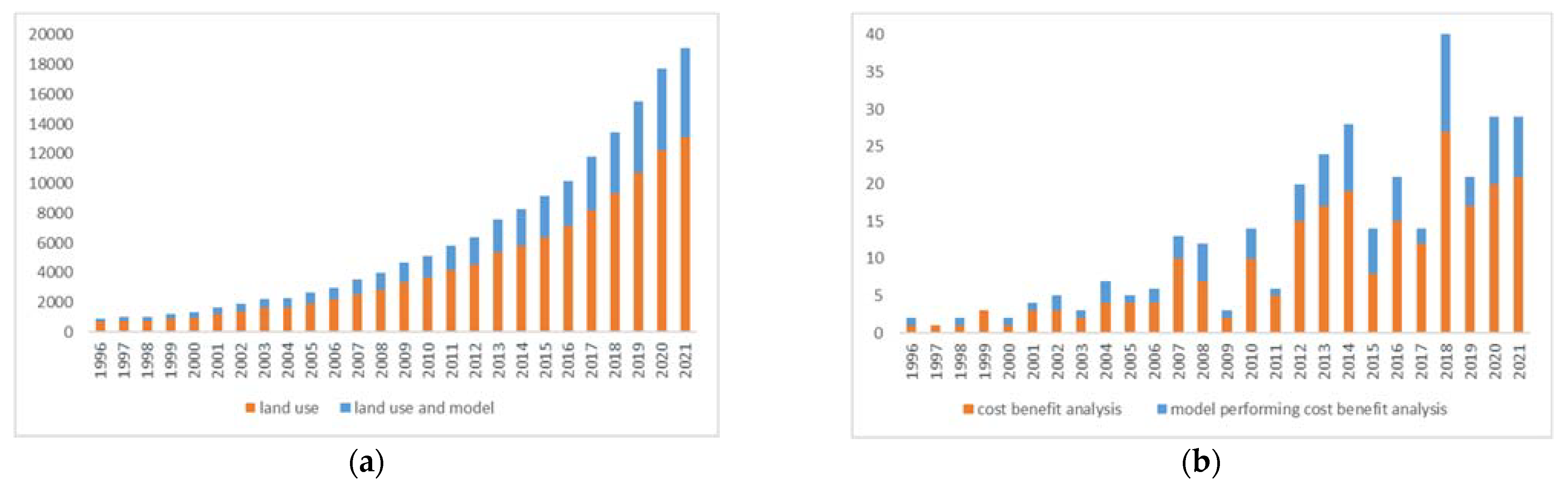
2. Literature Search
3. Results and Discussion
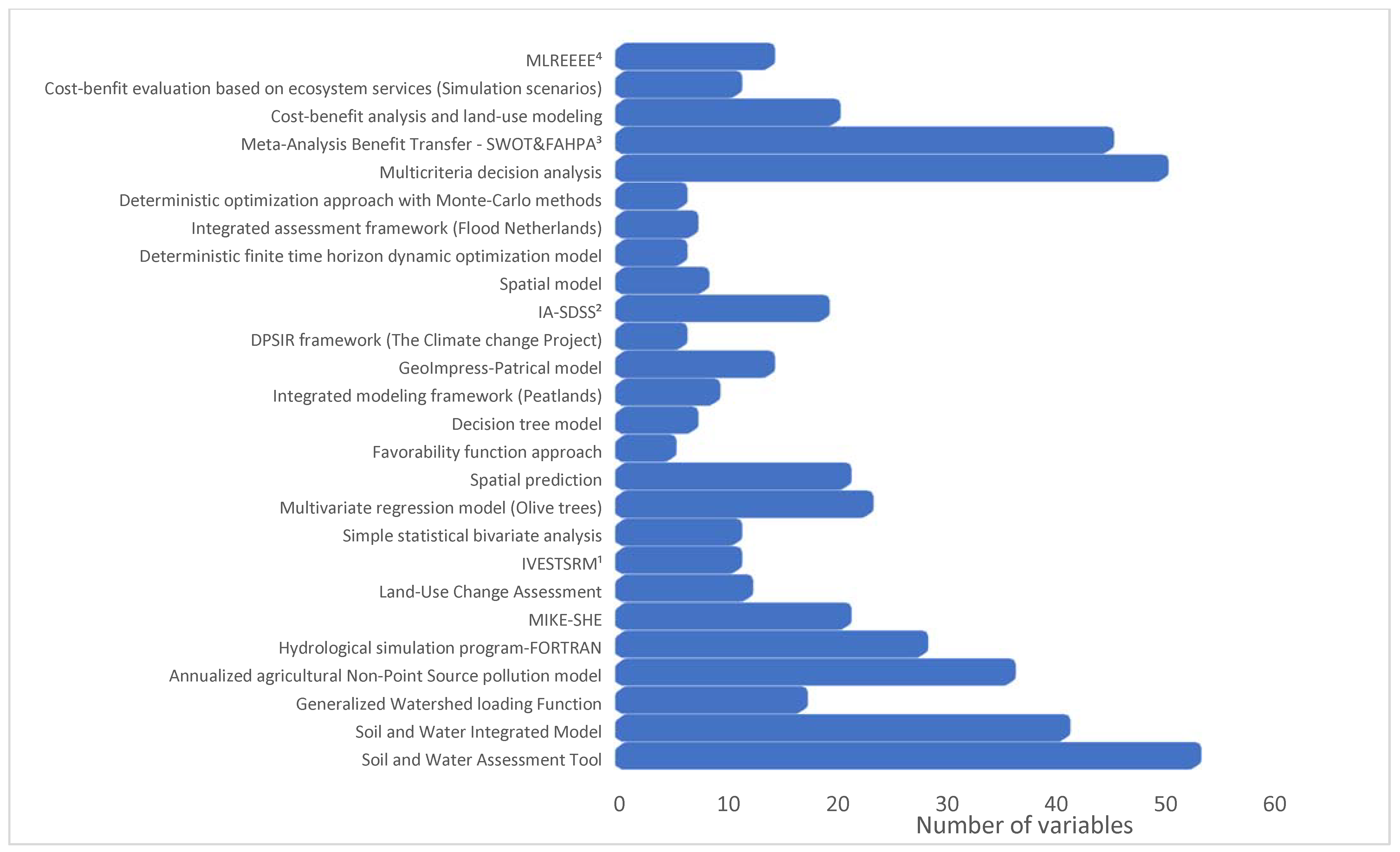
3.1. Analysis of Selected Land-Use-Based Models
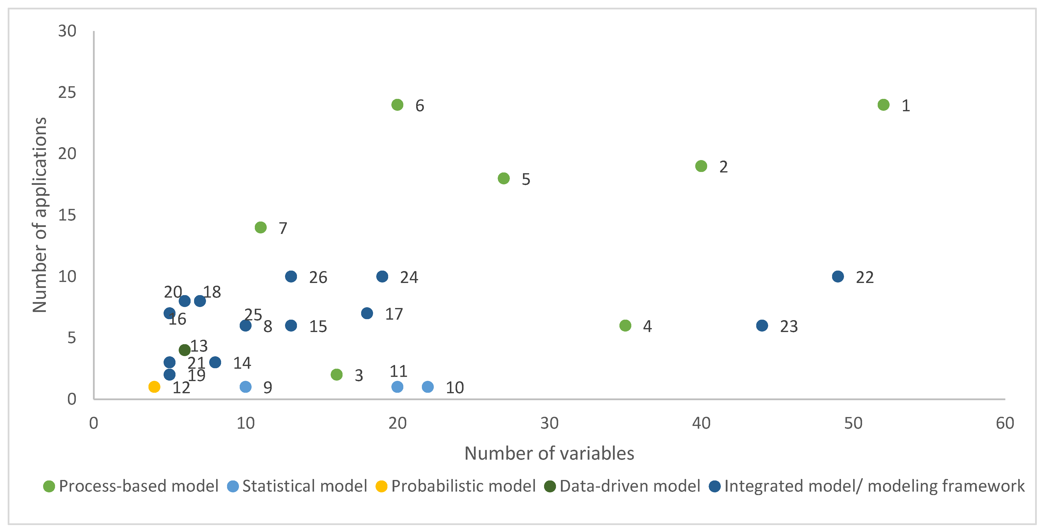
3.1.1. Input Variables and Data Needed
3.1.2. User Convenience
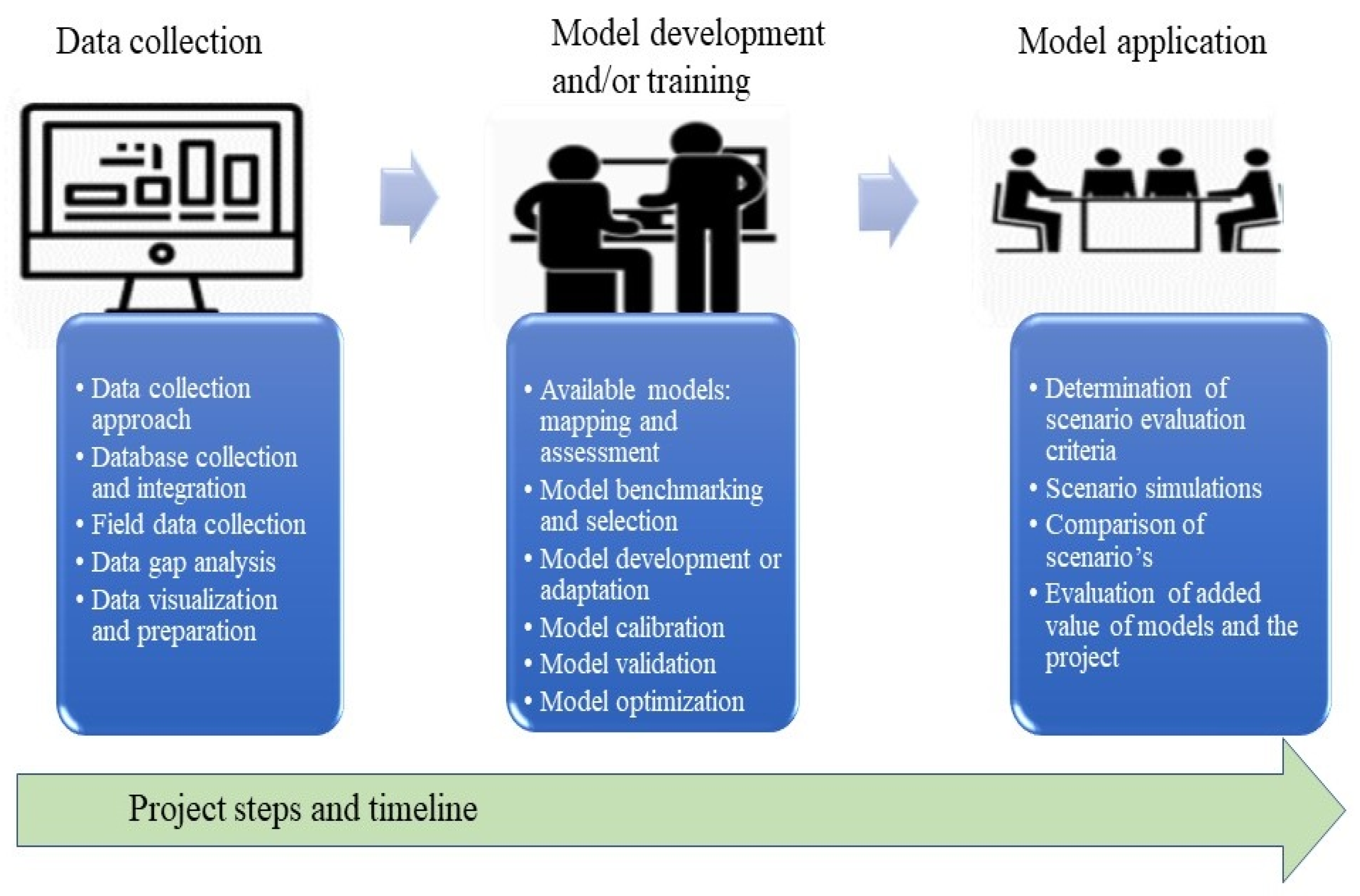
3.2. Steps in Modeling
3.2.1. Data Collection
3.2.2. Model Development and/or Training
3.2.3. Model Application
3.3. SWOT Analysis
3.3.1. Strengths
3.3.2. Weaknesses
3.3.3. Opportunities
3.3.4. Threats
3.4. River Basin Models in the Context of Sustainable River Basin Management
4. Conclusions
Supplementary Materials
Author Contributions
Funding
Institutional Review Board Statement
Informed Consent Statement
Data Availability Statement
Conflicts of Interest
References
- Foley, J.A.; DeFries, R.; Asner, G.P.; Barford, C.; Bonan, G.; Carpenter, S.R.; Chapin, F.S.; Coe, M.T.; Daily, G.C.; Gibbs, H.K. Global consequences of land use. Science 2005, 309, 570–574. [Google Scholar] [CrossRef] [PubMed] [Green Version]
- Hölting, L.; Beckmann, M.; Volk, M.; Cord, A.F. Multifunctionality assessments–More than assessing multiple ecosystem functions and services? A quantitative literature review. Ecol. Indic. 2019, 103, 226–235. [Google Scholar] [CrossRef]
- Auzins, A.; Geipele, I.; Stamure, I. Measuring land-use efficiency in land management. Adv. Mater. Res. 2013, 804, 205–210. [Google Scholar] [CrossRef]
- Laurance, W.F.; Cochrane, M.A.; Bergen, S.; Fearnside, P.M.; Delamônica, P.; Barber, C.; D’angelo, S.; Fernandes, T. The future of the Brazilian Amazon. Science 2001, 291, 438–439. [Google Scholar] [CrossRef] [PubMed] [Green Version]
- Ellis, E.C.; Wang, S. Sustainable traditional agriculture in the Tai Lake Region of China. Agric. Ecosyst. Environ. 1997, 61, 177–193. [Google Scholar] [CrossRef]
- Forio, M.A.E.; Villa-Cox, G.; Van Echelpoel, W.; Ryckebusch, H.; Lock, K.; Spanoghe, P.; Deknock, A.; De Troyer, N.; Nolivos-Alvarez, I.; Dominguez-Granda, L.; et al. Bayesian Belief Network models as trade-off tools of ecosystem services in the Guayas River Basin in Ecuador. Ecosyst. Serv. 2020, 44, 101124. [Google Scholar] [CrossRef]
- Gonzalez-Redin, J.; Luque, S.; Poggio, L.; Smith, R.; Gimona, A. Spatial Bayesian belief networks as a planning decision tool for mapping ecosystem services trade-offs on forested landscapes. Environ. Res. 2016, 144, 15–26. [Google Scholar] [CrossRef]
- Cord, A.F.; Bartkowski, B.; Beckmann, M.; Dittrich, A.; Hermans-Neumann, K.; Kaim, A.; Lienhoop, N.; Locher-Krause, K.; Priess, J.; Schröter-Schlaack, C.; et al. Towards systematic analyses of ecosystem service trade-offs and synergies: Main concepts, methods and the road ahead. Ecosyst. Serv. 2017, 28, 264–272. [Google Scholar] [CrossRef]
- Tilman, D.; Fargione, J.; Wolff, B.; D’antonio, C.; Dobson, A.; Howarth, R.; Schindler, D.; Schlesinger, W.H.; Simberloff, D.; Swackhamer, D. Forecasting agriculturally driven global environmental change. Science 2001, 292, 281–284. [Google Scholar] [CrossRef] [Green Version]
- Vitousek, P.M.; Mooney, H.A.; Lubchenco, J.; Melillo, J.M. Human domination of Earth’s ecosystems. Science 1997, 277, 494–499. [Google Scholar] [CrossRef] [Green Version]
- Matson, P.A.; Parton, W.J.; Power, A.G.; Swift, M.J. Agricultural intensification and ecosystem properties. Science 1997, 277, 504–509. [Google Scholar] [CrossRef] [PubMed] [Green Version]
- Wackernagel, M.; Schulz, N.B.; Deumling, D.; Linares, A.C.; Jenkins, M.; Kapos, V.; Monfreda, C.; Loh, J.; Myers, N.; Norgaard, R. Tracking the ecological overshoot of the human economy. Proc. Natl. Acad. Sci. USA 2002, 99, 9266–9271. [Google Scholar] [CrossRef] [PubMed] [Green Version]
- Pielke Sr, R.A.; Marland, G.; Betts, R.A.; Chase, T.N.; Eastman, J.L.; Niles, J.O.; Niyogi, D.D.S.; Running, S.W. The influence of land-use change and landscape dynamics on the climate system: Relevance to climate-change policy beyond the radiative effect of greenhouse gases. Philos. Trans. R. Soc. London. Ser. A Math. Phys. Eng. Sci. 2002, 360, 1705–1719. [Google Scholar] [CrossRef] [PubMed]
- Vörösmarty, C.J.; Green, P.; Salisbury, J.; Lammers, R.B. Global water resources: Vulnerability from climate change and population growth. Science 2000, 289, 284–288. [Google Scholar] [CrossRef] [Green Version]
- Postel, S.L.; Daily, G.C.; Ehrlich, P.R. Human appropriation of renewable fresh water. Science 1996, 271, 785–788. [Google Scholar] [CrossRef]
- Bennett, E.M.; Carpenter, S.R.; Caraco, N.F. Human impact on erodable phosphorus and eutrophication: A global perspective: Increasing accumulation of phosphorus in soil threatens rivers, lakes, and coastal oceans with eutrophication. BioScience 2001, 51, 227–234. [Google Scholar] [CrossRef]
- Pearce, D.W.; Nash, C. The Social Appraisal of Projects: A Text in Cost-Benefit Analysis; Halsted Press: Sydney, Australia, 1981. [Google Scholar] [CrossRef]
- Dixon, J.A.; Hufschmidt, M.M. Economic Valuation Techniques for the Environment; a Case Study Workbook; Johns Hopkins Univ. Press: Baltimore, MD, USA, 1986. [Google Scholar]
- De Groot, R.S.; Alkemade, R.; Braat, L.; Hein, L.; Willemen, L. Challenges in integrating the concept of ecosystem services and values in landscape planning, management and decision making. Ecol. Complex. 2010, 7, 260–272. [Google Scholar] [CrossRef]
- Boardman, A.E.; Greenberg, D.H.; Vining, A.R.; Weimer, D.L. Cost-Benefit Analysis: Concepts and Practice; Cambridge University Press: Cambridge, UK, 2018. [Google Scholar]
- Levin, H.; Belfield, C. Cost-benefit analysis and cost-effectiveness analysis. Educ. Econ. 2010, 5, 197–201. [Google Scholar]
- Jeswani, H.K.; Azapagic, A.; Schepelmann, P.; Ritthoff, M. Options for broadening and deepening the LCA approaches. J. Clean. Prod. 2010, 18, 120–127. [Google Scholar] [CrossRef]
- Venkatachalam, L. The contingent valuation method: A review. Environ. Impact Assess. Rev. 2004, 24, 89–124. [Google Scholar] [CrossRef]
- Atkinson, G.; Mourato, S. Environmental cost-benefit analysis. Annu. Rev. Environ. Resour. 2008, 33, 317–344. [Google Scholar] [CrossRef]
- Newcomer, K.E.; Hatry, H.P.; Wholey, J.S. Cost-effectiveness and cost-benefit analysis. In Handbook of Practical Program Evaluation, Fourth; Wiley Online Library: Hoboken, NJ, USA, 2015; pp. 636–672. [Google Scholar] [CrossRef]
- Brouwer, R.; Van Ek, R. Integrated ecological, economic and social impact assessment of alternative flood control policies in the Netherlands. Ecol. Econ. 2004, 50, 1–21. [Google Scholar] [CrossRef]
- DeAngelis, D.L.; Yurek, S. Spatially explicit modeling in ecology: A review. Ecosystems 2017, 20, 284–300. [Google Scholar] [CrossRef]
- Jakeman, A.J.; El Sawah, S.; Guillaume, J.H.; Pierce, S.A. Making progress in integrated modelling and environmental decision support. In Proceedings of the International Symposium on Environmental Software Systems, Wageningen, The Netherlands, 5–7 February 2017; pp. 15–25. [Google Scholar]
- Fatichi, S.; Vivoni, E.R.; Ogden, F.L.; Ivanov, V.Y.; Mirus, B.; Gochis, D.; Downer, C.W.; Camporese, M.; Davison, J.H.; Ebel, B. An overview of current applications, challenges, and future trends in distributed process-based models in hydrology. J. Hydrol. 2016, 537, 45–60. [Google Scholar] [CrossRef] [Green Version]
- Hutson, J.; Correll, R. Easy to Use Pesticide Fate/Effects Models and Statistical Tools. In Integrated Analytical Approaches for Pesticide Management; Elsevier: Amsterdam, The Netherlands, 2018; pp. 185–196. [Google Scholar]
- Solomatine, D.; See, L.M.; Abrahart, R. Data-driven modelling: Concepts, approaches and experiences. Pract. Hydroinformatics 2009, 68, 17–30. [Google Scholar]
- Solomatine, D.P.; Ostfeld, A. Data-driven modelling: Some past experiences and new approaches. J. Hydroinformatics 2008, 10, 3–22. [Google Scholar] [CrossRef] [Green Version]
- Ruokolainen, L.; Lindén, A.; Kaitala, V.; Fowler, M.S. Ecological and evolutionary dynamics under coloured environmental variation. Trends Ecol. Evol. 2009, 24, 555–563. [Google Scholar] [CrossRef]
- Guisan, A.; Zimmermann, N.E. Predictive habitat distribution models in ecology. Ecol. Model. 2000, 135, 147–186. [Google Scholar] [CrossRef]
- Everaert, G.; Holguin Gonzalez, J.; Goethals, P. Selecting relevant predictors: Impact of variable selection on model performance, uncertainty and applicability of models in environmental decision making. In Proceedings of the 6th Biannial meeting of the International Environmental Modelling and Software Society (iEMSs 2012): Managing resources of a limited planet: Pathways and visions under uncertainty, Leipzig, Germany, 11 January 2012; pp. 1603–1611. [Google Scholar]
- Forio, M.A.E.; Mouton, A.; Lock, K.; Boets, P.; Nguyen, T.H.T.; Ambarita, M.N.D.; Musonge, P.L.S.; Dominguez-Granda, L.; Goethals, P.L. Fuzzy modelling to identify key drivers of ecological water quality to support decision and policy making. Environ. Sci. Policy 2017, 68, 58–68. [Google Scholar] [CrossRef]
- Zuur, A.F.; Ieno, E.N.; Elphick, C.S. A protocol for data exploration to avoid common statistical problems. Methods Ecol. Evol. 2010, 1, 3–14. [Google Scholar] [CrossRef]
- Tuo, Y.; Chiogna, G.; Disse, M. A Multi-Criteria Model Selection Protocol for Practical Applications to Nutrient Transport at the Catchment Scale. Water 2015, 7, 2851–2880. [Google Scholar] [CrossRef] [Green Version]
- Sun, L.; Lu, W.; Yang, Q.; Martín, J.D.; Li, D. Ecological Compensation Estimation of Soil and Water Conservation Based on Cost-Benefit Analysis. Water Resour. Manag. 2013, 27, 2709–2727. [Google Scholar] [CrossRef]
- Strehmel, A.; Schmalz, B.; Fohrer, N. Evaluation of land use, land management and soil conservation strategies to reduce non-point source pollution loads in the three gorges region, China. Environ. Manag. 2016, 58, 906–921. [Google Scholar] [CrossRef]
- Liu, R.; Zhang, P.; Wang, X.; Wang, J.; Yu, W.; Shen, Z. Cost-effectiveness and cost-benefit analysis of BMPs in controlling agricultural nonpoint source pollution in China based on the SWAT model. Environ. Monit. Assess. 2014, 186, 9011–9022. [Google Scholar] [CrossRef] [PubMed]
- Rocha, J.; Roebeling, P.; Rial-Rivas, M.E. Assessing the impacts of sustainable agricultural practices for water quality improvements in the Vouga catchment (Portugal) using the SWAT model. Sci. Total Environ. 2015, 536, 48–58. [Google Scholar] [CrossRef] [PubMed]
- Mtibaa, S.; Hotta, N.; Irie, M. Analysis of the efficacy and cost-effectiveness of best management practices for controlling sediment yield: A case study of the Joumine watershed, Tunisia. Sci. Total Environ. 2018, 616–617, 1–16. [Google Scholar] [CrossRef]
- Thorsen, M.; Refsgaard, J.; Hansen, S.; Pebesma, E.; Jensen, J.; Kleeschulte, S. Assessment of uncertainty in simulation of nitrate leaching to aquifers at catchment scale. J. Hydrol. 2001, 242, 210–227. [Google Scholar] [CrossRef]
- Liu, H.; Yi, Y.; Blagodatsky, S.; Cadisch, G. Impact of forest cover and conservation agriculture on sediment export: A case study in a montane reserve, south-western China. Sci. Total Environ. 2020, 702, 134802. [Google Scholar] [CrossRef]
- Udayakumara, E.P.N.; Gunawardena, P. Modelling soil erosion and hydropower linkages of Rantambe reservoir, Sri Lanka: Towards payments for ecosystem services. Modeling Earth Syst. Environ. 2022, 8, 1617–1634. [Google Scholar] [CrossRef]
- Conforti, M.; Robustelli, G.; Muto, F.; Critelli, S. Application and validation of bivariate GIS-based landslide susceptibility assessment for the Vitravo river catchment (Calabria, south Italy). Nat. Hazards 2012, 61, 127–141. [Google Scholar] [CrossRef]
- Noori, O.; Panda, S.S. Site-specific management of common olive: Remote sensing, geospatial, and advanced image processing applications. Comput. Electron. Agric. 2016, 127, 680–689. [Google Scholar] [CrossRef]
- Qiu, Y.; Fu, B.-j.; Wang, J.; Chen, L.; Meng, Q.; Zhang, Y. Spatial prediction of soil moisture content using multiple-linear regressions in a gully catchment of the Loess Plateau, China. J. Arid Environ. 2010, 74, 208–220. [Google Scholar] [CrossRef]
- Chung, C.-J.F.; Fabbri, A.G. Validation of spatial prediction models for landslide hazard mapping. Nat. Hazards 2003, 30, 451–472. [Google Scholar] [CrossRef]
- Crossman, N.D.; Connor, J.D.; Bryan, B.A.; Summers, D.M.; Ginnivan, J. Reconfiguring an irrigation landscape to improve provision of ecosystem services. Ecol. Econ. 2010, 69, 1031–1042. [Google Scholar] [CrossRef]
- Van Hardeveld, H.; Driessen, P.; Schot, P.; Wassen, M. An integrated modelling framework to assess long-term impacts of water management strategies steering soil subsidence in peatlands. Environ. Impact Assess. Rev. 2017, 66, 66–77. [Google Scholar] [CrossRef]
- Ferrer, J.; Pérez-Martín, M.A.; Jiménez, S.; Estrela, T.; Andreu, J. GIS-based models for water quantity and quality assessment in the Júcar River Basin, Spain, including climate change effects. Sci. Total Environ. 2012, 440, 42–59. [Google Scholar] [CrossRef] [PubMed]
- Pouget, L.; Escaler, I.; Guiu, R.; Mc Ennis, S.; Versini, P.A. Global Change adaptation in water resources management: The Water Change project. Sci. Total Environ. 2012, 440, 186–193. [Google Scholar] [CrossRef]
- Wang, J.; Chen, J.; Ju, W.; Li, M. IA-SDSS: A GIS-based land use decision support system with consideration of carbon sequestration. Environ. Model. Softw. 2010, 25, 539–553. [Google Scholar] [CrossRef]
- Zarei, A.; Dadashpoor, H.; Amini, M. Determination of the optimal land use allocation pattern in Nowshahr County, Northern Iran. Environ. Dev. Sustain. 2016, 18, 37–56. [Google Scholar] [CrossRef]
- Cerdá, E.; Martín-Barroso, D. Optimal control for forest management and conservation analysis in dehesa ecosystems. Eur. J. Oper. Res. 2013, 227, 515–526. [Google Scholar] [CrossRef]
- Monge, J.J.; Daigneault, A.J.; Dowling, L.J.; Harrison, D.R.; Awatere, S.; Ausseil, A.-G. Implications of future climatic uncertainty on payments for forest ecosystem services: The case of the East Coast of New Zealand. Ecosyst. Serv. 2018, 33, 199–212. [Google Scholar] [CrossRef]
- Mwambo, F.M.; Fürst, C.; Nyarko, B.K.; Borgemeister, C.; Martius, C. Maize production and environmental costs: Resource evaluation and strategic land use planning for food security in northern Ghana by means of coupled emergy and data envelopment analysis. Land Use Policy 2020, 95, 104490. [Google Scholar] [CrossRef]
- Jahanifar, K.; Amirnejad, H.; Azadi, H.; Adenle, A.A.; Scheffran, J. Economic analysis of land use changes in forests and rangelands: Developing conservation strategies. Land Use Policy 2019, 88, 104003. [Google Scholar] [CrossRef]
- Pan, Y.; Wu, J.; Zhang, Y.; Zhang, X.; Yu, C. Simultaneous enhancement of ecosystem services and poverty reduction through adjustments to subsidy policies relating to grassland use in Tibet, China. Ecosyst. Serv. 2021, 48, 101254. [Google Scholar] [CrossRef]
- Li, M.; Liu, S.; Liu, Y.; Sun, Y.; Wang, F.; Dong, S.; An, Y. The cost–benefit evaluation based on ecosystem services under different ecological restoration scenarios. Environ. Monit. Assess. 2021, 193, 398. [Google Scholar] [CrossRef]
- Bertoni, D.; Aletti, G.; Cavicchioli, D.; Micheletti, A.; Pretolani, R. Estimating the CAP greening effect by machine learning techniques: A big data ex post analysis. Environ. Sci. Policy 2021, 119, 44–53. [Google Scholar] [CrossRef]
- Goethals, P.L.; Forio, M.A.E. Advances in ecological water system modeling: Integration and leanification as a basis for application in environmental management. Water 2018, 10, 1219. [Google Scholar] [CrossRef] [Green Version]
- Guo, Y.; Fang, G.; Xu, Y.-P.; Tian, X.; Xie, J. Identifying how future climate and land use/cover changes impact streamflow in Xinanjiang Basin, East China. Sci. Total Environ. 2020, 710, 136275. [Google Scholar] [CrossRef]
- Box, G.E.; Draper, N.R. Empirical Model-Building and Response Surfaces; John Wiley & Sons, Inc.: Hoboken, NJ, USA, 1986; Volume 424. [Google Scholar]
- Catchment Hydrology, C. Series on Model Choice: 1: General Approaches to Modelling and Practical Issues of Model Choice. Cooperative Research Centre for Catchment Hydrology, 2005. Available online: https://scholar.google.be/scholar?hl=en&as_sdt=0%2C5&q=Catchment+Hydrology%2C+C.+Series+on+model+choice%3A+1%3A+General+approaches+to+modelling+and+practical+issues+of+model+choice.+Cooperative+Research+Centre+for+Catchment+Hydrology&btnG= (accessed on 15 July 2022).
- Bertrand-Krajewski, J.-L. Stormwater pollutant loads modelling: Epistemological aspects and case studies on the influence of field data sets on calibration and verification. Water Sci. Technol. 2007, 55, 1–17. [Google Scholar] [CrossRef]
- Michener, W.K.; Jones, M.B. Ecoinformatics: Supporting ecology as a data-intensive science. Trends Ecol. Evol. 2012, 27, 85–93. [Google Scholar] [CrossRef] [Green Version]
- Porter, J.H.; Ramsey, K. Integrating ecological data: Tools and techniques. In Proceedings of the 6th World Multi-Conference on Systematics, Cybernetics and Informatics, Orlando, FL, USA, 14–18 July 2002; pp. 396–401. [Google Scholar]
- Kelling, S.; Hochachka, W.M.; Fink, D.; Riedewald, M.; Caruana, R.; Ballard, G.; Hooker, G. Data-intensive science: A new paradigm for biodiversity studies. BioScience 2009, 59, 613–620. [Google Scholar] [CrossRef]
- Hackett, E.J.; Parker, J.N.; Conz, D.; Rhoten, D.; Parker, A. Ecology transformed: NCEAS and changing patterns of ecological research. In Scientific Collaboration on the Internet; MIT Press: Cambridge, MA, USA, 2008; pp. 277–296. [Google Scholar]
- Weiss, D.J.; Atkinson, P.M.; Bhatt, S.; Mappin, B.; Hay, S.I.; Gething, P.W. An effective approach for gap-filling continental scale remotely sensed time-series. ISPRS J. Photogramm. Remote Sens. 2014, 98, 106–118. [Google Scholar] [CrossRef] [PubMed] [Green Version]
- Lerner, B.; Boose, E.; Osterweil, L.J.; Ellison, A.; Clarke, L. Provenance and quality control in sensor networks. In Proceedings of the Environmental Information Management Conference 2011 (EIM 2011), Santa Barbara, CA, USA, 28–29 September 2011; pp. 98–103. [Google Scholar]
- Missier, P.; Ludäscher, B.; Bowers, S.; Dey, S.; Sarkar, A.; Shrestha, B.; Altintas, I.; Anand, M.K.; Goble, C. Linking multiple workflow provenance traces for interoperable collaborative science. In Proceedings of the 5th Workshop on Workflows in Support of Large-Scale Science, New Orleans, LA, USA, 14 November 2010; pp. 1–8. [Google Scholar]
- Osterweil, L.J.; Clarke, L.A.; Ellison, A.M.; Boose, E.; Podorozhny, R.; Wise, A. Clear and precise specification of ecological data management processes and dataset provenance. IEEE Trans. Autom. Sci. Eng. 2009, 7, 189–195. [Google Scholar] [CrossRef] [Green Version]
- Moriasi, D.N.; Arnold, J.G.; Van Liew, M.W.; Bingner, R.L.; Harmel, R.D.; Veith, T.L. Model evaluation guidelines for systematic quantification of accuracy in watershed simulations. Trans. ASABE 2007, 50, 885–900. [Google Scholar] [CrossRef]
- Refsgaard, J.C. Parameterisation, calibration and validation of distributed hydrological models. J. Hydrol. 1997, 198, 69–97. [Google Scholar] [CrossRef]
- Engel, B.; Storm, D.; White, M.; Arnold, J.; Arabi, M. A hydrologic/water quality model Applicati1 1. JAWRA J. Am. Water Resour. Assoc. 2007, 43, 1223–1236. [Google Scholar] [CrossRef]
- Gan, T.Y.; Dlamini, E.M.; Biftu, G.F. Effects of model complexity and structure, data quality, and objective functions on hydrologic modeling. J. Hydrol. 1997, 192, 81–103. [Google Scholar] [CrossRef]
- Boyle, D.P.; Gupta, H.V.; Sorooshian, S. Toward improved calibration of hydrologic models: Combining the strengths of manual and automatic methods. Water Resour. Res. 2000, 36, 3663–3674. [Google Scholar] [CrossRef]
- Birattari, M.; Kacprzyk, J. Tuning Metaheuristics: A Machine Learning Perspective; Springer: Berlin/Heidelberg, Germany, 2009; Volume 197. [Google Scholar]
- Maher, M.; Sakr, S. Smartml: A meta learning-based framework for automated selection and hyperparameter tuning for machine learning algorithms. In Proceedings of the EDBT: 22nd International Conference on Extending Database Technology, Lisbon, Portugal, 26–29 March 2019. [Google Scholar]
- Schratz, P.; Muenchow, J.; Iturritxa, E.; Richter, J.; Brenning, A. Hyperparameter tuning and performance assessment of statistical and machine-learning algorithms using spatial data. Ecol. Model. 2019, 406, 109–120. [Google Scholar] [CrossRef] [Green Version]
- Loucks, D.P.; Van Beek, E. Water Resource Systems Planning and Management: An Introduction to Methods, Models, and Applications; Springer: Berlin/Heidelberg, Germany, 2017. [Google Scholar]
- Kishita, Y.; Hara, K.; Uwasu, M.; Umeda, Y. Research needs and challenges faced in supporting scenario design in sustainability science: A literature review. Sustain. Sci. 2016, 11, 331–347. [Google Scholar] [CrossRef]
- Greiner, R.; Puig, J.; Huchery, C.; Collier, N.; Garnett, S.T. Scenario modelling to support industry strategic planning and decision making. Environ. Model. Softw. 2014, 55, 120–131. [Google Scholar] [CrossRef] [Green Version]
- Schwarz, P. The Art of the Long View: Planning for the Future in an Uncertain World; Currency Doubleday Publisher: New York, NY, USA, 2012; Available online: https://books.google.be/books?hl=en&lr=&id=T-r36bIZA44C&oi=fnd&pg=PR13&dq=The+art+of+the+long+view:+planning+for+the+future+in+an+uncertain+world&ots=1T_gUrSYR0&sig=gjkk17nV0LHhE9HUJwYO6yrcjTY#v=onepage&q=The%20art%20of%20the%20long%20view%3A%20planning%20for%20the%20future%20in%20an%20uncertain%20world&f=false (accessed on 15 July 2022).
- Van der Heijden, K. Scenarios: The Art of Strategic Conversation; John Wiley & Sons: Hoboken, NJ, USA, 2011. [Google Scholar]
- Strauch, M.; Cord, A.F.; Pätzold, C.; Lautenbach, S.; Kaim, A.; Schweitzer, C.; Seppelt, R.; Volk, M. Constraints in multi-objective optimization of land use allocation—Repair or penalize? Environ. Model. Softw. 2019, 118, 241–251. [Google Scholar] [CrossRef]
- Ding, T.; Liang, L.; Zhou, K.; Yang, M.; Wei, Y. Water-energy nexus: The origin, development and prospect. Ecol. Model. 2020, 419, 108943. [Google Scholar] [CrossRef]
- Aguilera, P.A.; Fernández, A.; Fernández, R.; Rumí, R.; Salmerón, A. Bayesian networks in environmental modelling. Environ. Model. Softw. 2011, 26, 1376–1388. [Google Scholar] [CrossRef]
- Chan, T.U.; Hart, B.T.; Kennard, M.J.; Pusey, B.J.; Shenton, W.; Douglas, M.M.; Valentine, E.; Patel, S. Bayesian network models for environmental flow decision making in the Daly River, Northern Territory, Australia. River Res. Appl. 2012, 28, 283–301. [Google Scholar] [CrossRef]
- Nguyen, T.H.T.; Everaert, G.; Boets, P.; Forio, M.A.E.; Bennetsen, E.; Volk, M.; Hoang, T.H.T.; Goethals, P.L. Modelling tools to analyze and assess the ecological impact of hydropower dams. Water 2018, 10, 259. [Google Scholar] [CrossRef] [Green Version]
- Arnold, J.G.; Moriasi, D.N.; Gassman, P.W.; Abbaspour, K.C.; White, M.J.; Srinivasan, R.; Santhi, C.; Harmel, R.; Van Griensven, A.; Van Liew, M.W. SWAT: Model use, calibration, and validation. Trans. ASABE 2012, 55, 1491–1508. [Google Scholar] [CrossRef]
- Jacoub, G.; Westrich, B. Modelling transport dynamics of contaminated sediments in the headwater of a hydropower plant at the Upper Rhine River. Acta Hydrochim. Et Hydrobiol. 2006, 34, 279–286. [Google Scholar] [CrossRef]
- Li, R.; Chen, Q.; Duan, C. Ecological hydrograph based on Schizothorax chongi habitat conservation in the dewatered river channel between Jinping cascaded dams. Sci. China Technol. Sci. 2011, 54, 54–63. [Google Scholar] [CrossRef]
- Forio, M.A.; Goethals, P.L.M. An Integrated Approach of Multi-Community Monitoring and Assessment of Aquatic Ecosystems to Support Sustainable Development. Sustainability 2020, 12, 5603. [Google Scholar] [CrossRef]
- Goethals, P.L.; Dedecker, A.P.; Gabriels, W.; Lek, S.; De Pauw, N. Applications of artificial neural networks predicting macroinvertebrates in freshwaters. Aquat. Ecol. 2007, 41, 491–508. [Google Scholar] [CrossRef] [Green Version]
- Hoang, T.H.; Mouton, A.; Lock, K.; De Pauw, N.; Goethals, P.L. Integrating data-driven ecological models in an expert-based decision support system for water management in the Du river basin (Vietnam). Environ. Monit. Assess. 2013, 185, 631–642. [Google Scholar] [CrossRef] [PubMed]
- Boets, P.; Lock, K.; Messiaen, M.; Goethals, P.L. Combining data-driven methods and lab studies to analyse the ecology of Dikerogammarus villosus. Ecol. Inform. 2010, 5, 133–139. [Google Scholar] [CrossRef]


| Models | Data Needed | User Convenience | References | |
|---|---|---|---|---|
| Process-Based Models | ||||
| 1 | Soil and Water Assessment Tool | 52 | L | Tuo, et al. [38], Sun, et al. [39], Strehmel, et al. [40], Liu, et al. [41], Rocha, et al. [42], Mtibaa, et al. [43] |
| 2 | Soil and Water Integrated Model | 40 | L | Tuo, Chiogna and Disse [38] |
| 3 | Generalized Watershed loading Function | 16 | L | Tuo, Chiogna and Disse [38] |
| 4 | Annualized agricultural Non-Point Source pollution model | 35 | L | Tuo, Chiogna and Disse [38] |
| 5 | Hydrological simulation program-FORTRAN | 27 | L | Tuo, Chiogna and Disse [38] |
| 6 | MIKE-SHE | 20 | L | Thorsen, et al. [44] |
| 7 | Land Use Change Assessment | 11 | M | Liu, et al. [45] |
| 8 | Integrated Valuation of Ecosystem Services and Trade-offs Sediment Retention model | 10 | L | Udayakumara and Gunawardena [46] |
| Statistical models | ||||
| 9 | Simple statistical bivariate analysis | 10 | H | Conforti, et al. [47] |
| 10 | Multivariate regression model (Olive trees) | 22 | H | Noori and Panda [48] |
| 11 | Spatial prediction | 20 | H | Qiu, et al. [49] |
| Probabilistic models | ||||
| 12 | Favorability function approach | 4 | L | Chung and Fabbri [50] |
| Data-driven models | ||||
| 13 | Decision tree model | 6 | H | Crossman, et al. [51] |
| Integrated models/modeling frameworks | ||||
| 14 | Integrated modeling framework (peatlands) | 8 | L | Van Hardeveld, et al. [52] |
| 15 | GeoImpress-Patrical model | 13 | L | Ferrer, et al. [53] |
| 16 | DPSIR framework (The Climate change Project) | 5 | M | Pouget, et al. [54] |
| 17 | Integrated assessment framework and spatial decision support system (IA-SDSS) | 18 | L | Wang, et al. [55] |
| 18 | Spatial model | 7 | M | Zarei, et al. [56] |
| 19 | Deterministic finite time horizon dynamic optimization model | 5 | L | Cerdá and Martín-Barroso [57] |
| 20 | Integrated assessment framework (flood Netherlands) | 6 | M | Brouwer and Van Ek [26] |
| 21 | Deterministic optimization approach with Monte Carlo methods | 5 | L | Monge, et al. [58] |
| 22 | Multicriteria decision analysis | 49 | L | Mwambo, et al. [59] |
| 23 | Meta-Analysis Benefit Transfer—Strengths Weaknesses Opportunities Threats and Fuzzy Analytic Hierarchical process analysis | 44 | L | Jahanifar, et al. [60] |
| 24 | Cost-benefit analysis and land use modeling | 19 | L | Pan, et al. [61] |
| 25 | Cost-benefit evaluation based on ecosystem services (Simulation scenarios) | 10 | M | Li, et al. [62] |
| 26 | Multinomial logistic regression and environmental and economic effect estimations | 13 | H | Bertoni, et al. [63] |
| Strengths Expert knowledge and empirical data can be used Analyses of various (spatially explicit) scenarios Applicable to various scales Provides time and spatial-specific output Some models includes both economic and environmental costs and benefits | Weaknesses Lack of model validation Presence of errors in data Limited data availability Models are too complex and some are too simple Some models are unable to incorporate other factors affecting the spatial variables such as land use Assumptions (e.g., spatial generalization) are used for the estimation of economic impacts |
| Opportunities Spatial explicit models becoming more reliable Spatial data availability and quality are increasing Modeling is advancing The growing interest in river basin modeling | Threats Data collection is expensive Limited data availability Over or under prediction Results (e.g., land use changes) of some scenarios are unfeasible environmentally or/and economically |
Publisher’s Note: MDPI stays neutral with regard to jurisdictional claims in published maps and institutional affiliations. |
© 2022 by the authors. Licensee MDPI, Basel, Switzerland. This article is an open access article distributed under the terms and conditions of the Creative Commons Attribution (CC BY) license (https://creativecommons.org/licenses/by/4.0/).
Share and Cite
Ghafoor, J.; Forio, M.A.E.; Goethals, P.L.M. Spatially Explicit River Basin Models for Cost-Benefit Analyses to Optimize Land Use. Sustainability 2022, 14, 8953. https://doi.org/10.3390/su14148953
Ghafoor J, Forio MAE, Goethals PLM. Spatially Explicit River Basin Models for Cost-Benefit Analyses to Optimize Land Use. Sustainability. 2022; 14(14):8953. https://doi.org/10.3390/su14148953
Chicago/Turabian StyleGhafoor, Jawad, Marie Anne Eurie Forio, and Peter L. M. Goethals. 2022. "Spatially Explicit River Basin Models for Cost-Benefit Analyses to Optimize Land Use" Sustainability 14, no. 14: 8953. https://doi.org/10.3390/su14148953