
Solving the Green Open Vehicle Routing Problem Using a Membrane-Inspired Hybrid Algorithm


Abstract
:1. Introduction
- (1)
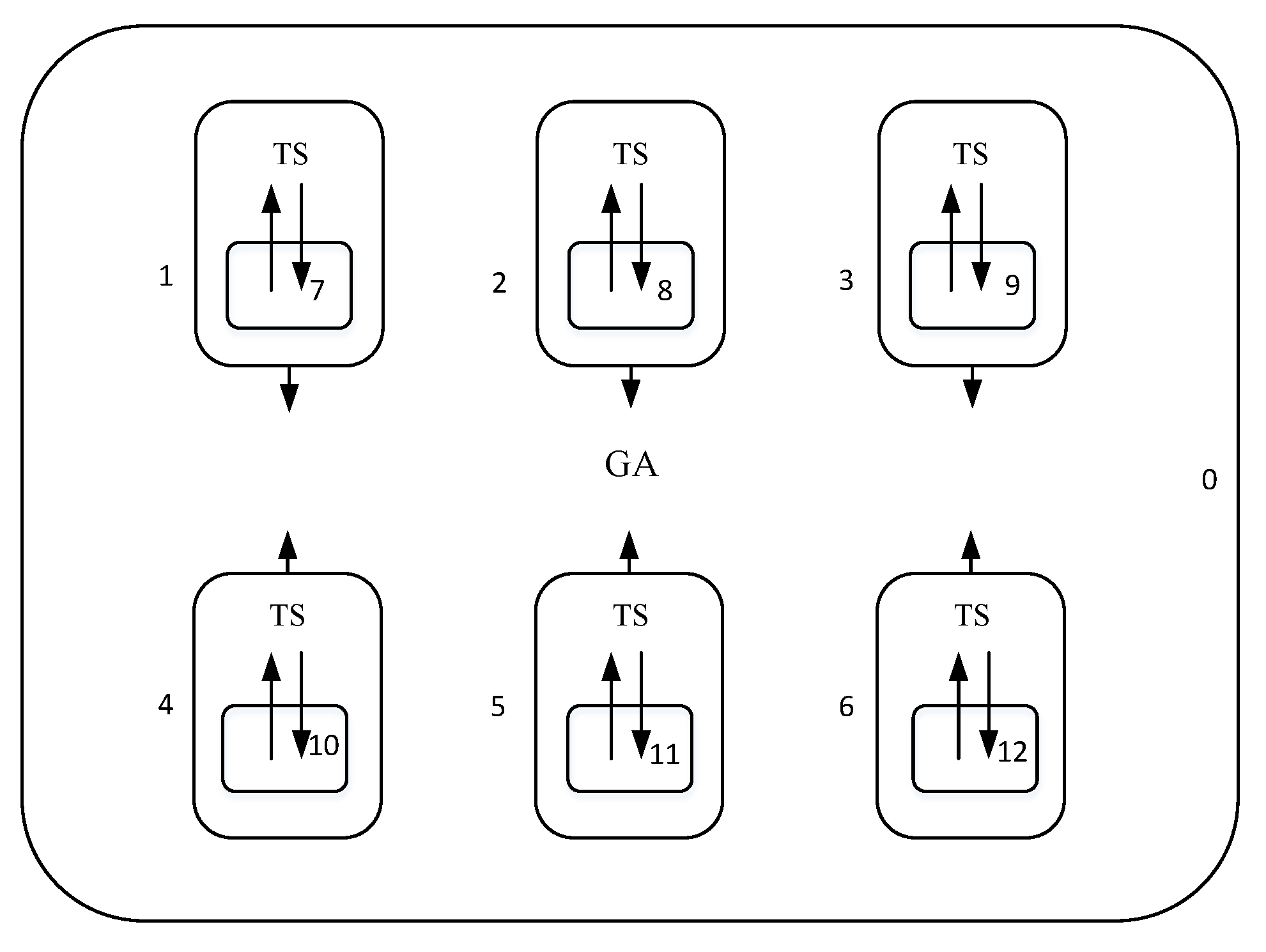
- A novel three-level nested membrane structure is designed with respective algorithms. To be specific, the skin membrane acts as the first level, where a genetic algorithm is mainly exploited to search for solutions to the routing problems. Six adjacent inner membranes act as the second level, where different tabu search algorithms are exploited to find tentative solutions. The elementary membrane in each level-2 membrane acts as the third level, where neighbourhood search operations are exploited to facilitate adjusting the search direction of the corresponding level-2 membrane.
- (2)
- Communication channels between the level-2 membranes and their inner membranes are designed to exchange solutions to favourably find better solutions. Communication channels also exist between the skin membrane and the level-2 membranes, where the crossover operator in the genetic operators is leveraged to retain satisfactory gene segments. In addition, the tabu search with different attractors is adopted to help the genetic algorithm escape from the local optimum. The convergence curve cliffs after each communication justify the effectiveness of the communication channels.
- (3)
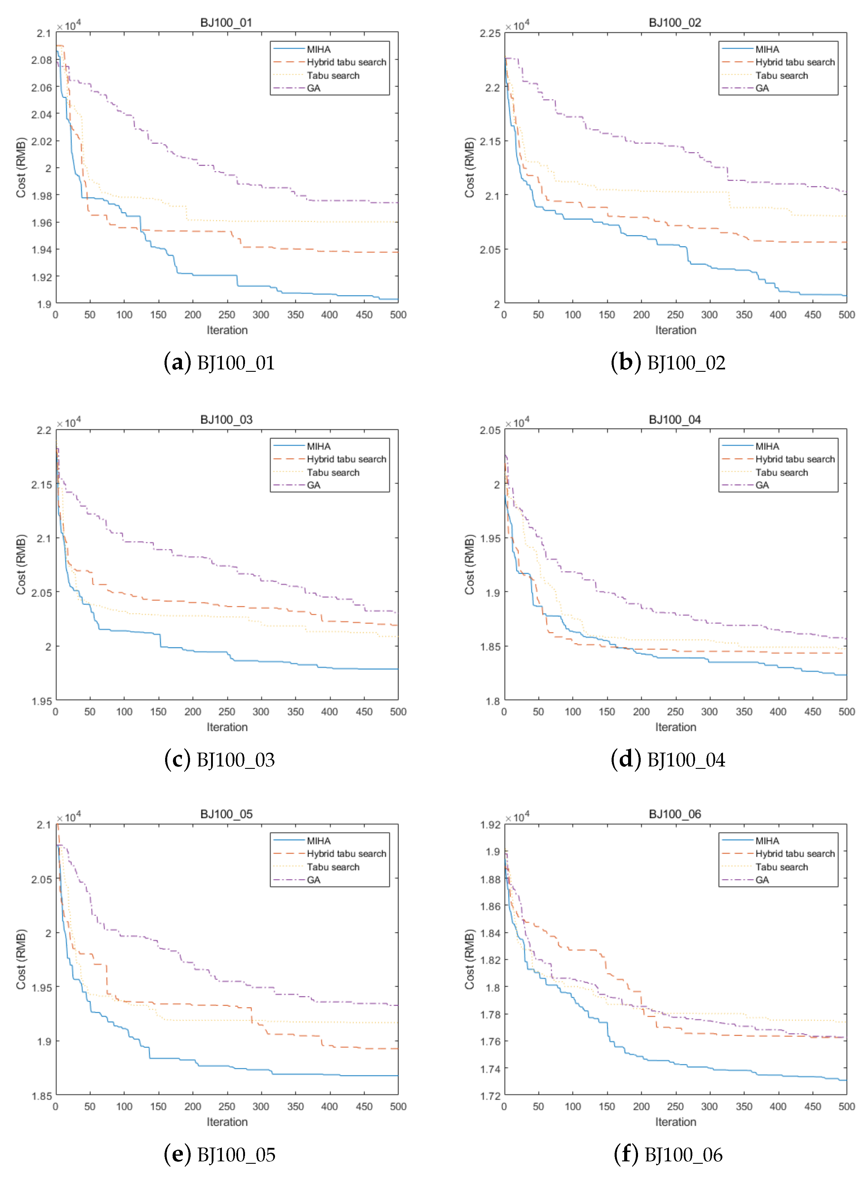
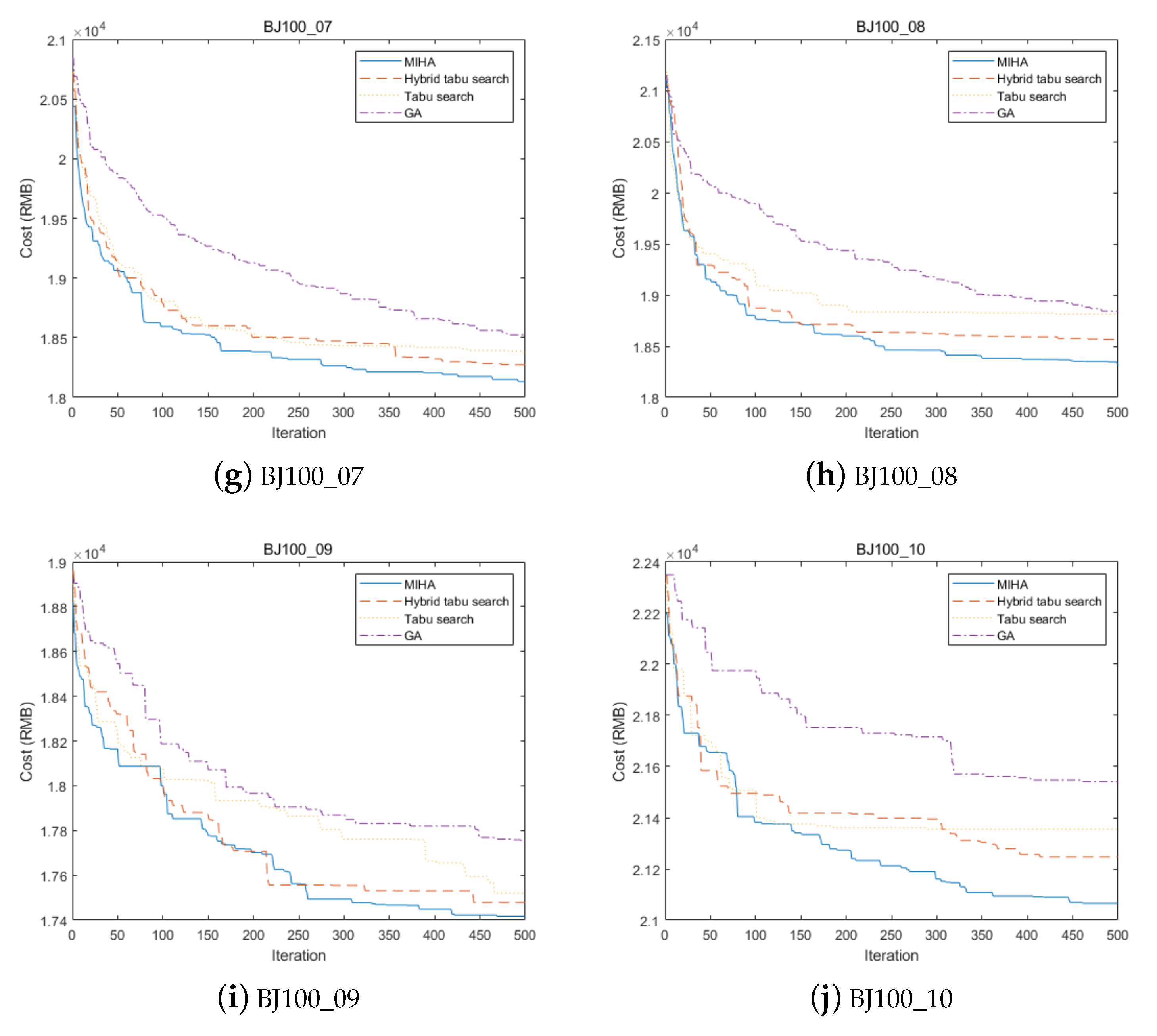
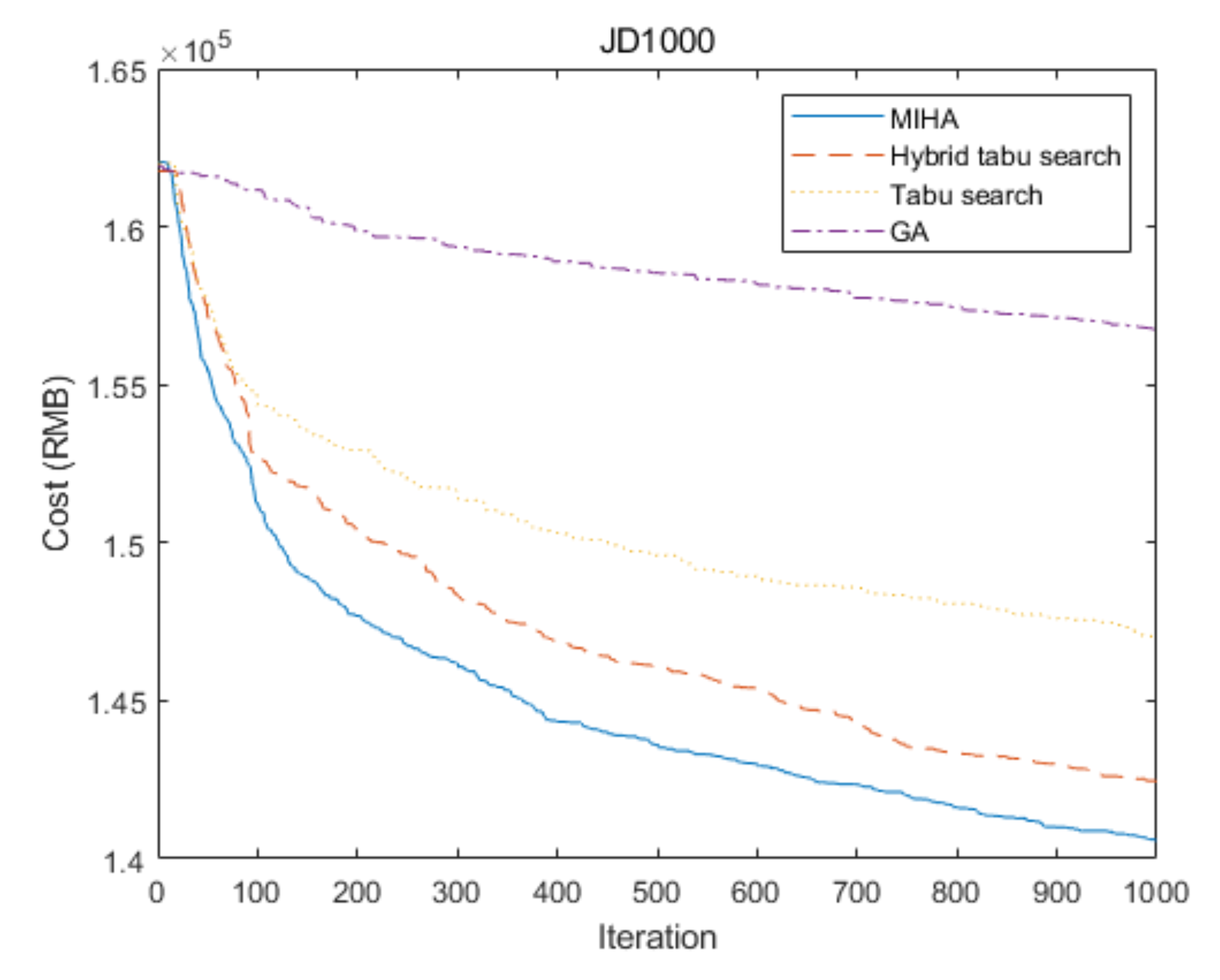
- Experiments are carried out on large-scale real-world problem instances, i.e., a Beijing 100-nodes set and a Jingdong 1000-nodes instance. The results demonstrate that our method significantly outperformed the hybrid tabu search [17], tabu search, and genetic algorithm, respectively. In particular, the computation time observed when comparing the performance on the Jingdong 1000-nodes instances and the Beijing 100-nodes instances further demonstrates the superiority of our algorithm in solving large-scale problems.
2. Related Work
2.1. Algorithms for the OVRP
2.2. Membrane Algorithms
3. Problem Formulation
4. The Proposed Method
| Algorithm 1 Pseudo-code of MIHA |
| Require: maximum number of iterations , iteration number before MCA |
| Ensure:. |
|
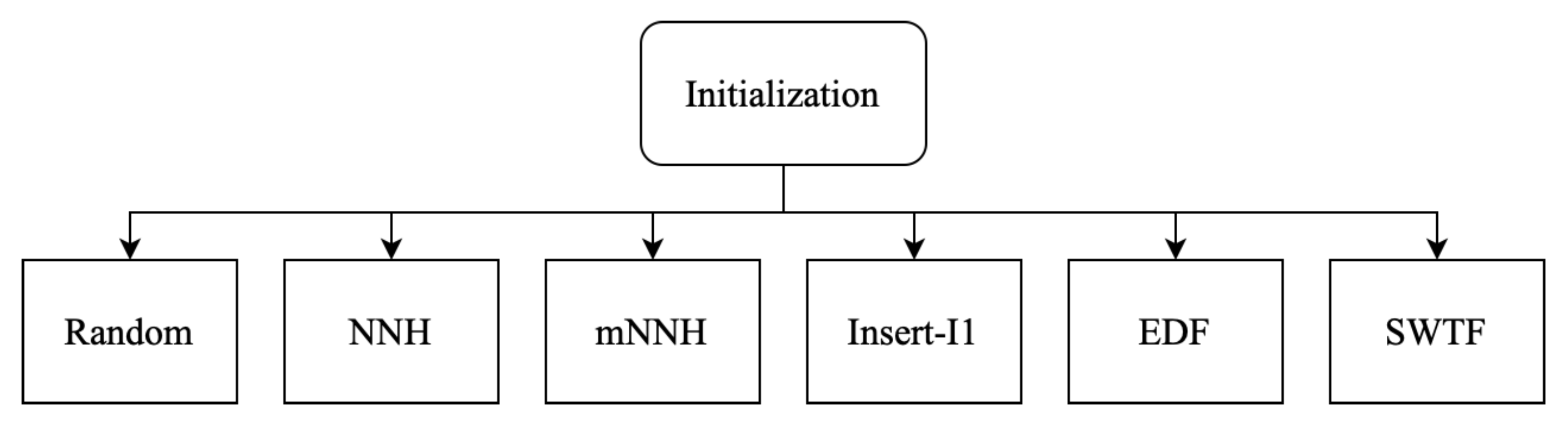
4.1. Initialisation
| Algorithm 2 Pseudo-code of initialisation |
| Require: Operators: Random, NNH, mNNH, , EDF, SWTF |
| Ensure: Implement the initialisation of MIHA |
|
- (1)
- Random heuristic: It randomly chooses routes that satisfy constraints (5)–(17).
- (2)
- Nearest neighbourhood heuristic (NNH): It generates a set of routes according to the distance from the current node. The nearest customer to the depot is chosen as the start node of the first route. Then it chooses an unassigned customer , who is nearest to . It repeats the same procedure until no feasible candidate nodes for the current route can be found. This also means that the current route is completed. Then, it allocates a new vehicle for the next route and constructs the route in a similar way until all customer nodes are assigned.
- (3)
- Modified nearest neighbourhood heuristic (mNNH): It generates a set of routes according to both the demand of the next customer and the distance from the current node. During the shipping process, a vehicle can offload payload after servicing customer i. The unit distance payload of customer j on arc is defined as . The mNNH creates a number of routes sequentially by considering the as an objective. First, it chooses the customer c that satisfies , where represents the unassigned customer set, which includes the initial current node of the first route. Next, the feasible customer that satisfies is selected as the next node c and added to the current route. Then, it repeats choosing the next node and appending it to the current route. If no more feasible nodes can be added, the current route is completed, and another route will be constructed in a similar way until all customers have been assigned.
- (4)
- Insert heuristic: As first proposed by Solomon [47], the customer is chosen based on the Equations (19) and (20) and then inserted to the route according to the insert heuristics. Moreover, the feasible and desired position of the selected in the route is decided by Equations (21) and (22) as follows, where is the new time for service to begin at customer j, given that u is on the route. The main idea is to use several criteria to insert a new customer into the current partial route at every iteration.
- (5)
- Earliest deadline first heuristic: It selects the customer with the earliest (or tightest) deadline for service at each step.
- (6)
- Shortest waiting time first heuristic: It selects the customer with the shortest waiting time.
4.2. GA in Skin Membrane
4.2.1. Crossover Operator
4.2.2. Mutation Operator
- (1)
- Random: This operation randomly removes a customer node from a given route and inserts it into another feasible position of the origin route.
- (2)
- Split-longest: This operation searches for the route with the highest total cost and breaks the route into two parts at a random point.
- (3)
- Merge-shortest: This operation searches for the two routes of the chromosome with the smallest total cost and appends one to the other.
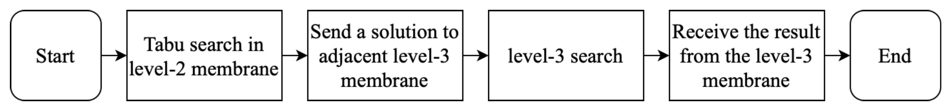
4.3. Tabu Search in Level-2 Membranes
| Algorithm 3 Level-2 Membrane Search Algorithm |
|
- (1)
- Random operator: It randomly exchanges the position of two nodes of a given solution, provided that no constraint is violated.
- (2)
- High-cost-node operator: It removes a high-cost customer node defined as , where i is the preceding customer and j is the succeeding customer, and inserts the node into another position.
- (3)
- Long-wait-time operator: It relocates the customer with a long wait time node defined as , where is the arrival time of customer u.
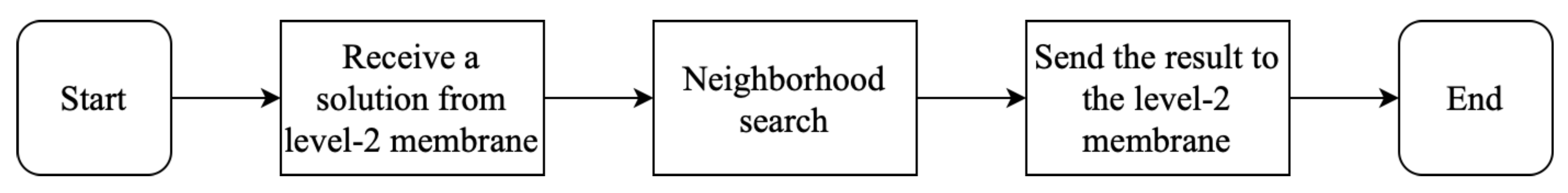
4.4. Neighbourhood Search in Level-3 Membranes
| Algorithm 4 Level-3 Membrane Search Algorithm |
|
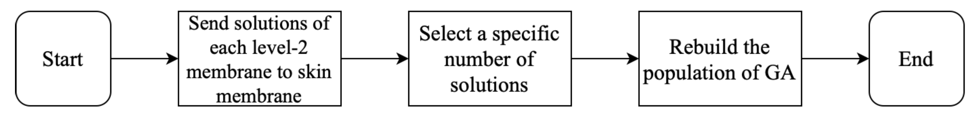
4.5. Communications between the Level-2 Membrane and Skin Membrane
| Algorithm 5 Membrane Communication Algorithm |
|
4.6. Speed Optimisation
| Algorithm 6 Speed and Departure-time Optimisation Algorithm (SDTOA) |
|
5. Computational Results
5.1. Parameter Analysis
5.1.1.
5.1.2.
5.2. Effectiveness of Search in Level-3 Membranes
5.3. Effectiveness of Tabu Search
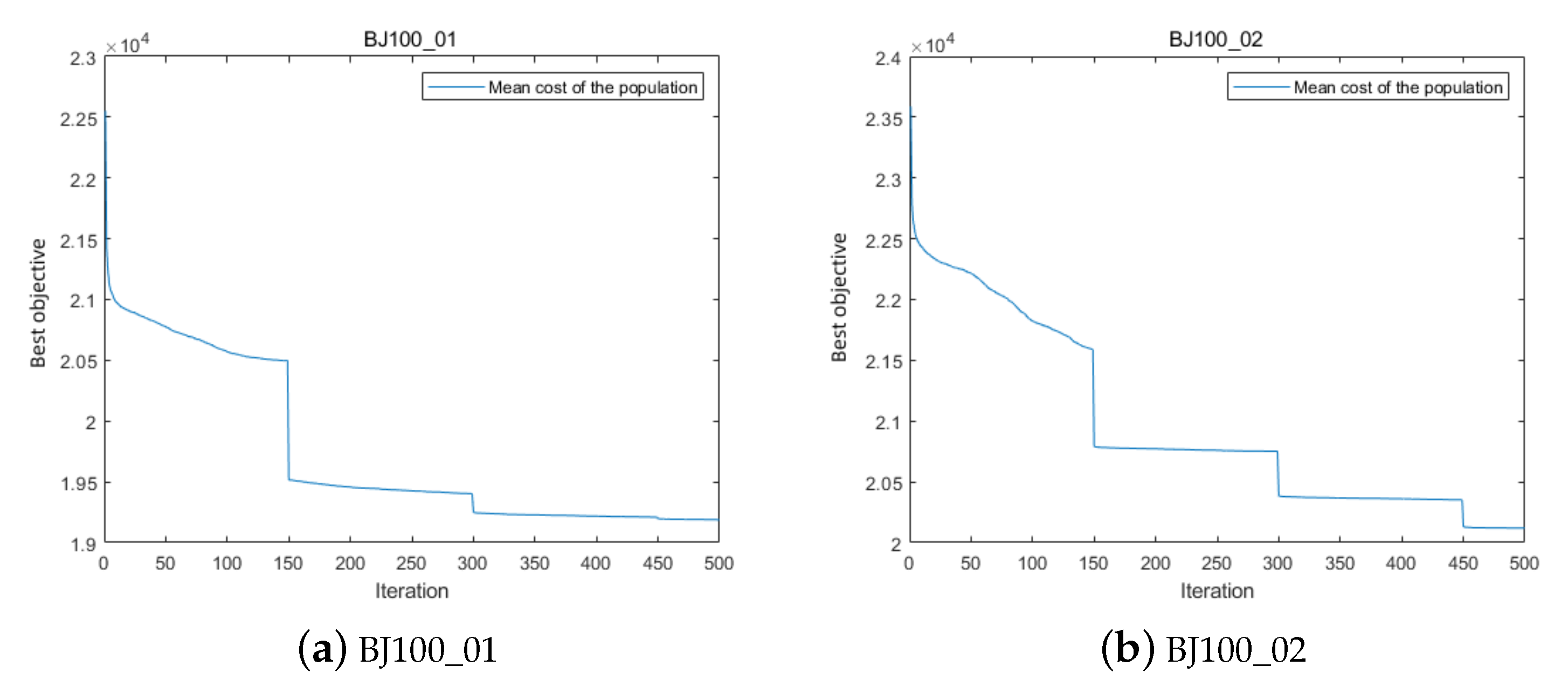
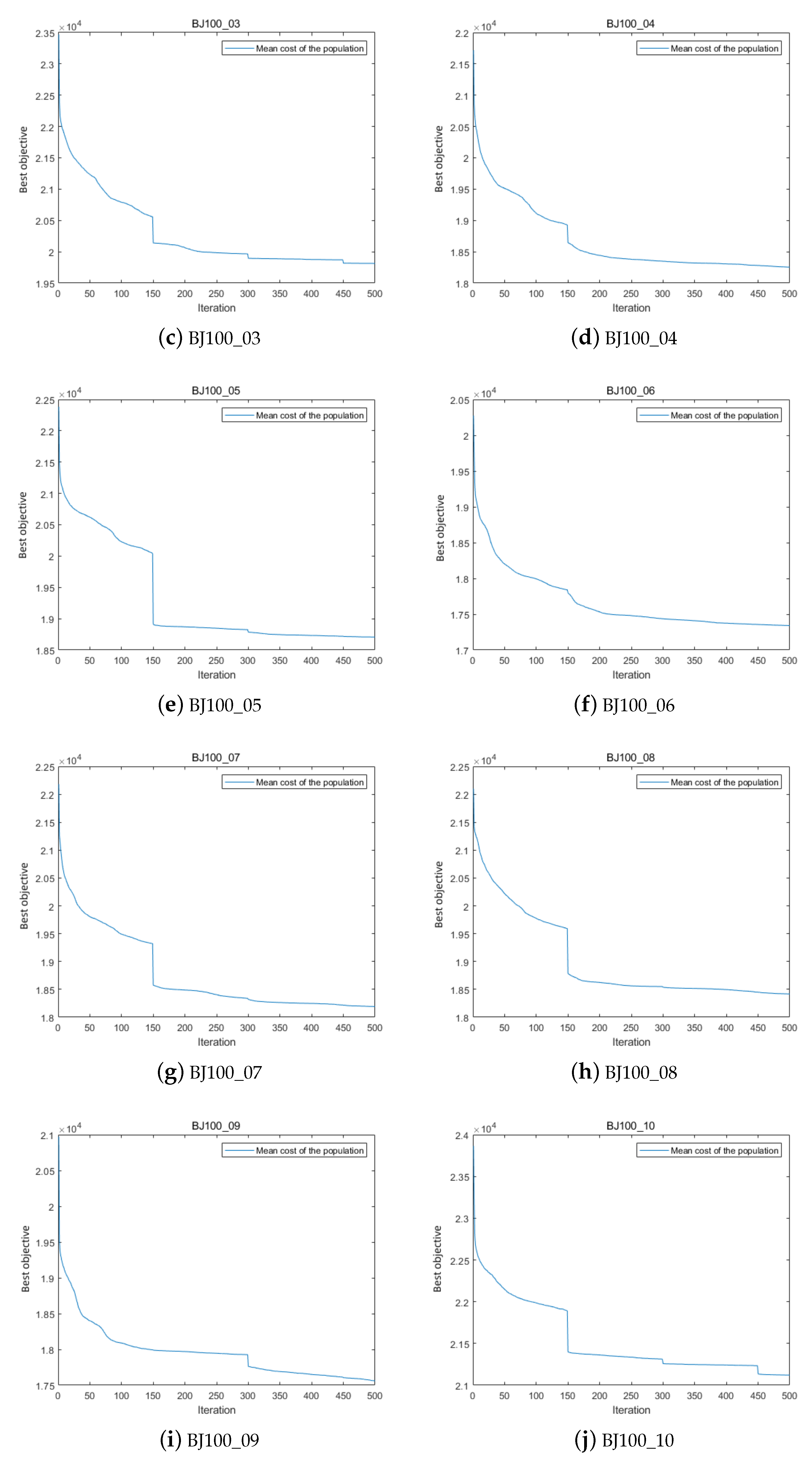
5.4. Effectiveness of GA in Skin Membrane
5.5. Effectiveness of the Membrane Structure
5.6. Computational Result of Larger-Scale Problems
5.7. Comparison with Other Algorithms
6. Conclusions
Author Contributions
Funding
Institutional Review Board Statement
Informed Consent Statement
Data Availability Statement
Conflicts of Interest
Notations
| G | Complete directed graph |
| N | Node set |
| Customer set | |
| A | Arc set |
| Q | Vehicle capacity |
| w | The weight of a vehicle |
| The demand of customer i | |
| The time cost of the route ending with i | |
| The actual starting time for serving node i | |
| The length of arc | |
| The amount of freight flow on arc | |
| Binary flag variable 1 | |
| Binary flag variable 2 | |
| The travel speed of vehicle r on arc | |
| The time window of customer i |
References
- Dantzig, G.B.; Ramser, R.H. The truck dispatching problem. Manag. Sci. 1959, 6, 80–91. [Google Scholar] [CrossRef]
- Long, J.; Sun, Z.; Pardalos, P.M.; Hong, Y.; Zhang, S.; Li, C. A hybrid multi-objective genetic local search algorithm for the prize-collecting vehicle routing problem. Inf. Sci. 2019, 478, 40–61. [Google Scholar] [CrossRef]
- Zhang, D.; Cai, S.; Ye, F.; Si, Y.; Nguyen, T.T. A hybrid algorithm for a vehicle routing problem with realistic constraints. Inf. Sci. 2017, 394, 167–182. [Google Scholar] [CrossRef]
- Toth, P.; Vigo, D. The Vehicle Routing Problem; Society for Industrial and Applied Mathematics: Philadelphia, PA, USA, 2002; p. 9. [Google Scholar]
- Repoussis, P.P.; Tarantilis, C.D.; Ioannou, G. The open vehicle routing problem with time windows. J. Oper. Res. 2007, 58, 355–367. [Google Scholar] [CrossRef]
- Moghdani, R.; Salimifard, K.; Demir, E.; Benyettou, A. The green vehicle routing problem: A systematic literature review. J. Clean. Prod. 2021, 279, 123691. [Google Scholar] [CrossRef]
- Bodin, L.; Golden, B.; Assad, A.; Ball, M. Routing and scheduling of vehicles and crews: The state of the art. Comput. Oper. Res. 1983, 10, 63–211. [Google Scholar]
- Brandao, J. A tabu search heuristic algorithm for open vehicle routing problem. Eur. J. Oper. Res. 2004, 157, 552–564. [Google Scholar] [CrossRef]
- Fleszar, K.; Osman, I.H.; Hindi, K.S. A variable neighbourhood search algorithm for the open vehicle routing problem. Eur. J. Oper. Res. 2009, 195, 803–809. [Google Scholar] [CrossRef]
- Tarantilis, C.D.; Ioannou, G.; Kiranoudis, C.T.; Prastacos, G.P. Solving the open vehicle routing problem via a single parameter meta-heuristic algorithm. J. Oper. Res. 2005, 56, 588–596. [Google Scholar] [CrossRef]
- MirHassani, S.; Abolghasemi, N. A particle swarm optimization algo-rithm for open vehicle routing problem. Expert Syst. Appl. 2011, 38, 11547–11551. [Google Scholar] [CrossRef]
- Li, X.; Tian, P.; Leung, S. An ant colony optimization metaheuristic hybridized with tabu search for the open vehicle routing problem. J. Oper. Res. Soc. 2009, 60, 1012–1025. [Google Scholar] [CrossRef]
- Repoussis, P.P.; Tarantilis, C.D.; Braysy, O.; Ioannou, G. A hybrid evolution strategy for the open vehicle routing problem. Comput. Oper. Res. 2010, 37, 443–455. [Google Scholar] [CrossRef]
- Ashtineh, H.; Pishvaee, M. Alternative Fuel Vehicle-Routing Problem: A life cycle analysis of transportation fuels. J. Clean. Prod. 2019, 219, 166–182. [Google Scholar] [CrossRef]
- Yu, Y.; Wang, S.; Wang, J.; Huang, M. A branch-and-price algorithm for the heterogeneous fleet green vehicle routing problem with time windows. Transp. Res. Part B Methodol. 2019, 122, 511–527. [Google Scholar] [CrossRef]
- Wang, L.; Lu, J. A memetic algorithm with competition for the capacitated green vehicle routing problem. IEEE/CAA J. Autom. Sin. 2019, 6, 516–526. [Google Scholar] [CrossRef]
- Niu, Y.; Yang, Z.; Chen, P.; Xiao, J. Optimizing the green open vehicle routing problem with time windows by minimizing comprehensive routing cost. J. Clean Prod. 2018, 171, 962–971. [Google Scholar] [CrossRef]
- Pan, L.; Păun, G.; Pérez-Jimxexnez, M.J. Spiking neural P systems with neuron division and budding. Sci. China Inf. Sci. 2011, 54, 1596–1607. [Google Scholar] [CrossRef] [Green Version]
- Păun, G. Computing with membranes. J. Comput. Syst. Sci. 2000, 61, 108–143. [Google Scholar] [CrossRef] [Green Version]
- Sosík, P. P systems attacking hard problems beyond NP: A survey. J. Membr. Comput. 2019, 1, 198–208. [Google Scholar] [CrossRef] [Green Version]
- Applications of Membrane Computing; Ciobanu, G.; Pérez-Jimxexnez, M.J.; Păun, G. (Eds.) Springer: Berlin/Heidelberg, Germany, 2006; Volume 287, pp. 73–100. [Google Scholar]
- Derigs, U.; Reuter, K. A simple and efficient tabu search heuristic for solving the open vehicle routing problem. J. Oper. Res. Soc. 2009, 60, 1658–1669. [Google Scholar] [CrossRef]
- Fu, Z.; Eglese, R.; Li, L. Corrigendum to the paper: A new tabu search heuristic for the open vehicle routing problem. J. Oper. Res. Soc. 2006, 57, 1017–1018. [Google Scholar] [CrossRef] [Green Version]
- Russell, R.; Chiang, W.; Zepeda, D. Integrating multi-product production and distribution in newspaper logistics. Comput. Oper. Res. 2008, 35, 1576–1588. [Google Scholar] [CrossRef]
- Pisinger, D.; Ropke, S. A general heuristic for vehicle routing problems. Comput. Oper. Res. 2007, 34, 2403–2435. [Google Scholar] [CrossRef]
- Salari, M.; Toth, P.; Tramontani, A. An ILP improvement procedure for the open vehicle routing problem. Comput. Oper. Res. 2010, 37, 2106–2120. [Google Scholar] [CrossRef] [Green Version]
- Zachariadis, E.; Kiranoudis, T. An open vehicle routing problem metaheuristic for examining wide solution neighbourhoods. Comput. Oper. Res. 2010, 37, 712–723. [Google Scholar] [CrossRef] [Green Version]
- Tarantilis, C.D.; Ioannou, G.; Kiranoudis, C.T.; Prastacos, G.P. A threshold accepting approach to the open vehicle routing problem. RAIRO Oper. Res. 2004, 38, 345–360. [Google Scholar] [CrossRef] [Green Version]
- Wang, W.; Wu, B.; Zhao, Y.; Feng, D. Particle swarm optimization for open vehicle routing problem. In International Conference on Intelligent Computing: Part II; Huang, D.S., Li, K., Irwin, G.W., Eds.; Springer: Berlin/Heidelberg, Germany, 2006; pp. 999–1007. [Google Scholar]
- Zhen, T.; Zhu, Y.; Zhang, Q. A particle swarm optimization algorithm for the open vehicle routing problem. In Proceedings of the 2009 International Conference on Environmental Science and Information Application Technology, Wuhan, China, 4–5 July 2009; pp. 560–563. [Google Scholar]
- Li, X.; Tian, P. An ant colony system for the open vehicle routing problem. In Lecture Notes in Computer Science (ANTS 2006); Dorigo, M., Ed.; Springer: Berlin/Heidelberg, Germany, 2006; Volume 4150, pp. 356–363. [Google Scholar]
- Pan, L.; Fu, Z. A clonal selection algorithm for open vehicle routing problem. In Proceedings of the 2009 Third International Conference on Genetic and Evolutionary Computing, Guilin, China, 14–17 October 2009; pp. 786–790. [Google Scholar]
- Yu, S.; Ding, C.; Zhu, K. A hybrid GA-TS algorithm for open routing optimization of coal mines material. Expert Syst. Appl. 2011, 38, 10568–10573. [Google Scholar] [CrossRef]
- Barbuti, R.; Bove, P.; Milazzo, P.; Pardini, G. Minimal probabilistic P systems for modelling ecological systems. Theor. Comput. Sci. 2015, 608, 36–56. [Google Scholar] [CrossRef]
- Lucie, C.; Erzsĕbet, C.; Ludxexk, C.; Petr, S. P colonies. J. Membr. Comput. 2019, 1, 178–197. [Google Scholar]
- Niu, Y.; Zhang, Y.; Zhang, J. Running cells with decision-making mechanism: Intelligence decision P System for evacuation simulation. Int. J. Comput. Commun. 2018, 13, 865–880. [Google Scholar] [CrossRef]
- Sakellariou, I.; Stamatopoulou, I.; Kefalas, P. Using membranes to model a multi-agent system towards underground metro station crowd behaviour simulation. In Proceedings of the ECAI 2012 Workshop, Montpellier, France, 28 August 2012; pp. 5–10. [Google Scholar]
- Nishida, T.Y. Membrane algorithms: Approximate algorithms for NP-complete optimization problems. In Applications of Membrane Computing; Springer: Berlin/Heidelberg, Germany, 2006; pp. 303–314. [Google Scholar]
- Zhang, G.; Liu, C.; Rong, H. Analyzing radar emitter signals with membrane algorithms. Math. Comput. Model. 2010, 52, 1997–2010. [Google Scholar] [CrossRef]
- Zhang, G.; Rong, H.; Neri, F.; Pérez-Jimxexnez, M.J. An optimization spiking neural P system for approximately solving combinatorial optimization problems. Int. J. Neural. Syst. 2014, 24, 1440006. [Google Scholar] [CrossRef] [PubMed]
- Zhang, G.; Rong, H.; Cheng, J.; Qin, Y. A population-membrane-system-inspired evolutionary algorithm for distribution network reconfiguration. J. Electron. 2014, 23, 437–441. [Google Scholar]
- Barth, M.; Boriboonsomsin, K. Energy and emissions impacts of a freeway-based dynamic eco-driving system. Transp. Res. Part D 2009, 14, 400–410. [Google Scholar] [CrossRef]
- Barth, M.; Younglove, T.; Scora, G. Development of a Heavy-Duty Diesel Modal Emissions and Fuel Consumption Model; Technical Report; UCB-ITSPRR-2005-1, California PATH Program; Institute of Transportation Studies, University of California at Berkeley: Berkeley, CA, USA, 2005. [Google Scholar]
- Scora, M.; Barth, G. Comprehensive Modal Emission Model (CMEM), Version 3.01, User Guide. Technical Report. 2006. Available online: http://www.cert.ucr.edu/cmem/docs/CMEM_User_Guide_v3.01d.pdf (accessed on 17 February 2014).
- Koç, Ç.; Bektaş, T.; Jabali, O.; Laporte, G. The fleet size and mix pollution-routing problem. Transp. Res. Part B Methodol. 2014, 70, 239–254. [Google Scholar] [CrossRef]
- Tan, K.C.; Cheong, C.K.; Goh, C.K. Solving multi-objective vehicle routing problem with stochastic demand via evolutionary computation. Eur. J. Oper. Res. 2007, 177, 813–839. [Google Scholar] [CrossRef]
- Solomon, M.M. Algorithms for the vehicle routing and scheduling problems with time window constraints. Oper. Res. 1987, 35, 254–265. [Google Scholar] [CrossRef] [Green Version]
- Kramer, M.; Maculan, N.; Subramanian, A.; Vidal, T. A speed and departure time optimization algorithm for the pollution-routing problem. Eur. J. Oper. Res. 2015, 247, 782–787. [Google Scholar] [CrossRef] [Green Version]
- Li, J.; Xin, L.; Cao, Z.; Lim, A.; Song, W.; Zhang, J. Heterogeneous Attentions for Solving Pickup and Delivery Problem via Deep Reinforcement Learning. IEEE Trans. Intell. Transp. Syst. 2021, 23, 2306–2315. [Google Scholar] [CrossRef]
- Wu, Y.; Song, W.; Cao, Z.; Zhang, J.; Lim, A. Learning Improvement Heuristics for Solving Routing Problems. IEEE Trans. Neural Netw. Learn. Syst. 2021, 1–13. [Google Scholar] [CrossRef]
- Xin, L.; Song, W.; Cao, Z.; Zhang, J. Step-wise deep learning models for solving routing problems. IEEE Trans. Ind. Inform. 2020, 17, 4861–4871. [Google Scholar] [CrossRef]
- Shi, C.; Zhang, Z.; Ji, C.; Li, X.; Di, L.; Wu, Z. Potential improvement in combustion and pollutant emissions of a hydrogen-enriched rotary engine by using novel recess configuration. Chemosphere 2022, 299, 134491. [Google Scholar] [CrossRef]
- Shi, C.; Ji, C.; Ge, Y.; Wang, S.; Wang, H.; Yang, J. Parametric analysis of hydrogen two-stage direct-injection on combustion characteristics, knock propensity, and emissions formation in a rotary engine. Fuel 2021, 287, 119418. [Google Scholar] [CrossRef]
- Menaga, D.; Revathi, S. Least lion optimisation algorithm (LLOA) based secret key generation for privacy preserving association rule hiding. IET Inf. Secur. 2018, 12, 332–340. [Google Scholar] [CrossRef]
- Fathollahi-Fard, A.M.; Hajiaghaei-Keshteli, M.; Tavakkoli-Moghaddam, R. Red deer algorithm (RDA): A new nature-inspired meta-heuristic. Soft Comput. 2020, 24, 14637–14665. [Google Scholar] [CrossRef]


| Notation | Description | Typical Value |
|---|---|---|
| Diesel engine efficiency | 0.45 | |
| Rolling resistance coefficient | 0.01 | |
| Density of air (kg/m) | 1.2041 | |
| Conversion factor (g/s to litre/s) | 737 | |
| Heating value of the typical diesel fuel (kilojoule/g) | 44 | |
| g | Constant of gravitation (m/s) | 9.81 |
| Vehicle drive train efficiency | 0.45 | |
| Fuel-to-air mass ratio | 1 | |
| Acceleration (m/s) | 0 | |
| Angle of the road | 0 | |
| Highest speed (m/s) | 27.8 (or 100 km/h) | |
| Lowest speed (m/s) | 5.5 (or 20 km/h) | |
| Cost of fuel and CO emissions (GBP/litre) | 1.4 | |
| Cost of driver wage (GBP/s) | 0.0022 | |
| Q | Vehicle capacity (kg) | 4000 |
| w | Vehicle curb weight (kg) | 3500 |
| f | Vehicle fixed cost (GBP/day) | 0 |
| V | Engine displacement (litre) | 4.5 |
| k | Engine friction factor (kilojoule/rev/litre) | 0.25 |
| Engine speed (rev/s) | 38.34 | |
| A | Area of frontal surface (m) | 7.0 |
| Aerodynamics drag coefficient | 0.6 |
| Notation | B | Typical Values |
|---|---|---|
| Iterations between MCAs | 150 | |
| Maximum iteration number | 500 | |
| Probability of level-3 search | 0.8 | |
| Archive size | 100 | |
| Neighbourhood size | 100 | |
| L | Tabu-list size | 30 |
| P | Population size | 100 |
| Rate of mutation | 0.8 | |
| Rate of crossover | 0.2 | |
| parameters |
| Best Solution | Mean Solution | Worst Solution | SD | ET | |
|---|---|---|---|---|---|
| 0 | 10,875.6553 | 10,928.4416 | 10,957.5933 | 22.3405 | 98.4386 |
| 0.1 | 10,882.5664 | 10,935.8356 | 10,978.9560 | 25.6220 | 99.7357 |
| 0.2 | 10,897.0627 | 10,922.4866 | 10,946.9486 | 14.2856 | 106.7122 |
| 0.3 | 10,894.6855 | 10,935.1849 | 10,981.7598 | 22.6840 | 114.1316 |
| 0.4 | 10,893.8999 | 10,927.5347 | 10,960.1311 | 20.8581 | 132.3853 |
| 0.5 | 10,870.5658 | 10,927.1250 | 10,965.2899 | 28.0809 | 139.0837 |
| 0.6 | 10,893.7139 | 10,922.8795 | 10,946.2359 | 19.7116 | 153.5391 |
| 0.7 | 10,859.4377 | 10,918.7540 | 10,956.2807 | 23.5941 | 158.2609 |
| 0.8 | 10,849.7328 | 10,907.9905 | 10,959.0818 | 28.7783 | 172.7458 |
| 0.9 | 10,885.8673 | 10,922.2359 | 10,945.8091 | 16.2176 | 172.7154 |
| 1 | 10,864.7334 | 10,914.4491 | 10,939.8273 | 21.2864 | 179.3093 |
| Best Solution | Mean Solution | Worst Solution | SD | ET | |
|---|---|---|---|---|---|
| 15 | 10,887.9339 | 10,915.9258 | 10,933.9978 | 12.4846 | 180.9297 |
| 25 | 10,887.3386 | 10,907.1512 | 10,946.9533 | 17.9590 | 179.3292 |
| 50 | 10,864.7334 | 10,914.4491 | 10,939.8273 | 21.2864 | 179.3093 |
| 75 | 10,887.7475 | 10,914.0151 | 10,947.0650 | 18.9695 | 175.5044 |
| 100 | 10,899.9133 | 10,917.2956 | 10,930.3250 | 9.1312 | 174.3383 |
| 125 | 10,881.1171 | 10,913.0205 | 10,956.5405 | 19.0231 | 180.1102 |
| 150 | 10,847.0901 | 10,900.6532 | 10,947.3101 | 26.0596 | 150.6687 |
| 175 | 10,866.3854 | 10,908.5777 | 10,944.5708 | 23.6946 | 158.3528 |
| 200 | 10,878.1705 | 10,911.7143 | 10,945.2829 | 18.0546 | 184.6337 |
| Instance | Best Solution | Mean Solution | Worst Solution | SD | ET | |
|---|---|---|---|---|---|---|
| MIHA | BJ60_01 | 10,864.7334 | 10,914.4491 | 10,939.8273 | 21.2864 | 179.3093 |
| BJ60_02 | 10,217.4691 | 10,310.1949 | 10,395.6818 | 54.3404 | 167.1625 | |
| BJ60_03 | 11,321.6848 | 11,423.8391 | 11,489.1644 | 53.3224 | 168.3861 | |
| BJ60_04 | 11,800.7563 | 11,847.7284 | 11,915.0534 | 31.7880 | 179.6456 | |
| BJ60_05 | 10,890.8377 | 10,909.8830 | 10,947.0117 | 14.5797 | 190.0507 | |
| BJ60_06 | 11,875.3018 | 11,916.5380 | 11,942.8835 | 21.5401 | 157.5884 | |
| BJ60_07 | 12,528.3080 | 12,634.5020 | 12,685.8953 | 54.0499 | 138.2126 | |
| BJ60_08 | 11,783.3490 | 11,867.4716 | 11,932.7904 | 45.1478 | 162.5045 | |
| BJ60_09 | 11,573.5410 | 11,705.3953 | 11,908.5312 | 107.6724 | 173.2149 | |
| BJ60_10 | 12,939.9900 | 13,196.1938 | 13,269.0754 | 90.2917 | 161.0214 | |
| Average | 11,579.5971 | 11,672.6195 | 11,742.5914 | 49.4019 | 167.7096 | |
| MIHA | BJ60_01 | 10,876.9472 | 10,929.2492 | 10,959.7533 | 23.8597 | 99.9533 |
| BJ60_02 | 10,354.6481 | 10,439.4020 | 10,529.0454 | 47.3483 | 98.3095 | |
| BJ60_03 | 11,417.6826 | 11,510.4497 | 11,651.4713 | 77.5482 | 99.3993 | |
| BJ60_04 | 11,810.6944 | 11,850.3646 | 11,947.2880 | 36.0053 | 104.0135 | |
| BJ60_05 | 10,900.3834 | 10,930.1086 | 10,996.6298 | 29.6276 | 115.6167 | |
| BJ60_06 | 11,884.6734 | 11,934.8017 | 11,994.1760 | 37.2390 | 100.8201 | |
| BJ60_07 | 12,570.4124 | 12,737.4635 | 12,916.3772 | 116.3777 | 88.5942 | |
| BJ60_08 | 11,816.6496 | 11,865.4873 | 11,937.1039 | 42.1579 | 94.7336 | |
| BJ60_09 | 11,652.5596 | 11,744.5783 | 11,860.8162 | 74.2931 | 92.3574 | |
| BJ60_10 | 13168.2194 | 13,240.3696 | 13,322.1267 | 43.8999 | 85.6219 | |
| Average | 11,645.2870 | 11,718.2275 | 11,811.4788 | 52.8356 | 97.9418 |
| Instance | Best Solution | Mean Solution | Worst Solution | SD | ET | |
|---|---|---|---|---|---|---|
| MIHA | BJ60_01 | 10,864.7334 | 10,914.4491 | 10,939.8273 | 21.2864 | 179.3093 |
| BJ60_02 | 10,217.4691 | 10,310.1949 | 10,395.6818 | 54.3404 | 167.1625 | |
| BJ60_03 | 11,321.6848 | 11,423.8391 | 11,489.1644 | 53.3224 | 168.3861 | |
| BJ60_04 | 11,800.7563 | 11,847.7284 | 11,915.0534 | 31.7880 | 179.6456 | |
| BJ60_05 | 10,890.8377 | 10,909.8830 | 10,947.0117 | 14.5797 | 190.0507 | |
| BJ60_06 | 11,875.3018 | 11,916.5380 | 11,942.8835 | 21.5401 | 157.5884 | |
| BJ60_07 | 12,528.3080 | 12,634.5020 | 12,685.8953 | 54.0499 | 138.2126 | |
| BJ60_08 | 11,783.3490 | 11,867.4716 | 11,932.7904 | 45.1478 | 162.5045 | |
| BJ60_09 | 11,573.5410 | 11,705.3953 | 11,908.5312 | 107.6724 | 173.2149 | |
| BJ60_10 | 12,939.9900 | 13,196.1938 | 13,269.0754 | 90.2917 | 161.0214 | |
| Average | 11,579.5971 | 11,672.6195 | 11,742.5914 | 49.4019 | 167.7096 | |
| MIHA | BJ60_01 | 10,887.9165 | 10,928.7764 | 10,958.6152 | 22.1538 | 179.1811 |
| BJ60_02 | 10,350.4335 | 10,433.3471 | 10,569.4033 | 66.3863 | 165.9635 | |
| BJ60_03 | 11,410.8506 | 11,546.6879 | 11,693.6700 | 83.6334 | 183.0199 | |
| BJ60_04 | 11,808.0504 | 11,876.0743 | 12,002.3412 | 60.3121 | 190.7105 | |
| BJ60_05 | 10,893.5351 | 10,908.2957 | 10,941.6042 | 15.4682 | 213.1253 | |
| BJ60_06 | 11,930.4763 | 11,993.7405 | 12,040.6174 | 29.2162 | 162.8483 | |
| BJ60_07 | 12,790.4131 | 12,945.8023 | 13,093.2836 | 95.8863 | 150.9155 | |
| BJ60_08 | 11,840.7762 | 11,980.0637 | 12,070.6884 | 64.6119 | 170.2074 | |
| BJ60_09 | 11,700.6390 | 12,040.8509 | 12,195.6716 | 140.5182 | 169.8237 | |
| BJ60_10 | 13,352.3191 | 13,452.7316 | 13,528.2388 | 54.9095 | 152.6279 | |
| Average | 11,696.5410 | 11,810.6370 | 11,909.4134 | 63.3096 | 173.8423 |
| Instance | Best Solution | Mean Solution | Worst Solution | SD | ET | |
|---|---|---|---|---|---|---|
| MIHA | BJ60_01 | 10,864.7334 | 10,914.4491 | 10,939.8273 | 21.2864 | 179.3093 |
| BJ60_02 | 10,217.4691 | 10,310.1949 | 10,395.6818 | 54.3404 | 167.1625 | |
| BJ60_03 | 11,321.6848 | 11,423.8391 | 11,489.1644 | 53.3224 | 168.3861 | |
| BJ60_04 | 11,800.7563 | 11,847.7284 | 11,915.0534 | 31.7880 | 179.6456 | |
| BJ60_05 | 10,890.8377 | 10,909.8830 | 10,947.0117 | 14.5797 | 190.0507 | |
| BJ60_06 | 11,875.3018 | 11,916.5380 | 11,942.8835 | 21.5401 | 157.5884 | |
| BJ60_07 | 12,528.3080 | 12,634.5020 | 12,685.8953 | 54.0499 | 138.2126 | |
| BJ60_08 | 11,783.3490 | 11,867.4716 | 11,932.7904 | 45.1478 | 162.5045 | |
| BJ60_09 | 11,573.5410 | 11,705.3953 | 11,908.5312 | 107.6724 | 173.2149 | |
| BJ60_10 | 12,939.9900 | 13,196.1938 | 13,269.0754 | 90.2917 | 161.0214 | |
| Average | 11,579.5971 | 11,672.6195 | 11,742.5914 | 49.4019 | 167.7096 | |
| MIHA | BJ60_01 | 10,889.6733 | 10,920.5130 | 10,947.4318 | 20.3041 | 162.6233 |
| BJ60_02 | 10,267.1195 | 10,333.7142 | 10,415.6234 | 49.4848 | 149.6058 | |
| BJ60_03 | 11,349.3097 | 11,473.1526 | 11,595.0291 | 77.7908 | 149.0490 | |
| BJ60_04 | 11,804.8311 | 11,843.4759 | 11,937.9748 | 39.7545 | 150.1856 | |
| BJ60_05 | 10,898.5533 | 10,917.0069 | 10,942.3023 | 14.3160 | 168.1142 | |
| BJ60_06 | 11,882.7327 | 11,939.8357 | 11,973.6663 | 30.1972 | 170.9655 | |
| BJ60_07 | 12,534.6436 | 12,658.8725 | 12,849.5941 | 85.0550 | 129.9516 | |
| BJ60_08 | 11,806.8383 | 11,876.4740 | 11,934.8815 | 39.6358 | 138.7723 | |
| BJ60_09 | 11,630.3241 | 11,687.7664 | 11,850.7900 | 63.9084 | 140.8432 | |
| BJ60_10 | 13,120.3543 | 13,262.1483 | 13,355.0285 | 75.4520 | 128.9989 | |
| Average | 11,618.4380 | 11,691.2960 | 11,780.2322 | 49.5899 | 148.9109 |
| Instance | Best Solution | Mean Solution | Worst Solution | SD | ET | |
|---|---|---|---|---|---|---|
| MIHA | BJ60_01 | 10,864.7334 | 10,914.4491 | 10,939.8273 | 21.2864 | 179.3093 |
| BJ60_02 | 10,217.4691 | 10,310.1949 | 10,395.6818 | 54.3404 | 167.1625 | |
| BJ60_03 | 11,321.6848 | 11,423.8391 | 11,489.1644 | 53.3224 | 168.3861 | |
| BJ60_04 | 11,800.7563 | 11,847.7284 | 11,915.0534 | 31.7880 | 179.6456 | |
| BJ60_05 | 10,890.8377 | 10,909.8830 | 10,947.0117 | 14.5797 | 190.0507 | |
| BJ60_06 | 11,875.3018 | 11,916.5380 | 11,942.8835 | 21.5401 | 157.5884 | |
| BJ60_07 | 12,528.3080 | 12,634.5020 | 12,685.8953 | 54.0499 | 138.2126 | |
| BJ60_08 | 11,783.3490 | 11,867.4716 | 11,932.7904 | 45.1478 | 162.5045 | |
| BJ60_09 | 11,573.5410 | 11,705.3953 | 11,908.5312 | 107.6724 | 173.2149 | |
| BJ60_10 | 12,939.9900 | 13,196.1938 | 13,269.0754 | 90.2917 | 161.0214 | |
| Average | 11,579.5971 | 11,672.6195 | 11,742.5914 | 49.4019 | 167.7096 | |
| MIHA | BJ60_01 | 11,328.7061 | 11,450.7661 | 11,645.5626 | 102.4337 | 16.3996 |
| BJ60_02 | 10,706.7220 | 10,825.8266 | 10,952.4319 | 77.1375 | 16.0414 | |
| BJ60_03 | 12,036.9001 | 12,135.7632 | 12,194.5568 | 54.3717 | 15.1175 | |
| BJ60_04 | 12,367.3172 | 12,561.4857 | 12,854.7533 | 147.9147 | 17.2651 | |
| BJ60_05 | 11,232.0918 | 11,294.0261 | 11,371.0893 | 52.7390 | 16.8575 | |
| BJ60_06 | 12,288.4131 | 12,446.6655 | 12,589.8602 | 89.2907 | 16.7956 | |
| BJ60_07 | 13,243.3081 | 13,393.8310 | 13,479.3281 | 84.1279 | 13.8604 | |
| BJ60_08 | 12,172.4397 | 12,363.8495 | 12,507.0350 | 110.1176 | 13.1230 | |
| BJ60_09 | 12,293.5838 | 12,422.8764 | 12,574.3870 | 75.6798 | 14.9571 | |
| BJ60_10 | 13,356.4703 | 13,585.7384 | 13,783.8378 | 130.1142 | 13.2258 | |
| Average | 12,102.5952 | 12,248.0829 | 12,395.2842 | 92.3927 | 15.3643 |
| Instance | Best Solution | Mean Solution | Worst Solution | SD | ET |
|---|---|---|---|---|---|
| BJ100_01 | 19,067.0291 | 19,198.1247 | 19,286.2464 | 77.2545 | 177.5238 |
| BJ100_02 | 20,054.6213 | 20,212.3116 | 20,335.2703 | 79.4795 | 177.5122 |
| BJ100_03 | 19,611.4194 | 19,739.1057 | 19,807.4854 | 69.5798 | 187.4094 |
| BJ100_04 | 18,185.2382 | 18,288.2393 | 18,365.8098 | 66.8545 | 183.9430 |
| BJ100_05 | 18,450.2424 | 18,650.0880 | 18,721.6565 | 78.3719 | 177.8560 |
| BJ100_06 | 17,185.9916 | 17,292.5207 | 17,429.9383 | 100.3186 | 191.1868 |
| BJ100_07 | 18,018.7958 | 18,130.9018 | 18,231.9109 | 58.4036 | 203.7468 |
| BJ100_08 | 18,077.4404 | 18,245.1333 | 18,386.8610 | 102.6939 | 190.7556 |
| BJ100_09 | 17,317.3479 | 17,414.3330 | 17,513.4761 | 57.2721 | 181.7808 |
| BJ100_10 | 20,888.4245 | 20,996.4199 | 21,191.1938 | 87.1091 | 165.4292 |
| Average | 18,685.6551 | 18,816.7178 | 18,926.9849 | 77.7338 | 183.7144 |
| Algorithm | Best Solution | Mean Solution | Worst Solution | SD | ET |
|---|---|---|---|---|---|
| MIHA | 140,577.0284 | 141,085.6778 | 141,823.7589 | 365.4070 | 2331.9363 |
| Instance | BJ60 | BJ100 | JD1000 |
|---|---|---|---|
| ET | 150.6687 | 183.7144 | 2331.9363 |
Publisher’s Note: MDPI stays neutral with regard to jurisdictional claims in published maps and institutional affiliations. |
© 2022 by the authors. Licensee MDPI, Basel, Switzerland. This article is an open access article distributed under the terms and conditions of the Creative Commons Attribution (CC BY) license (https://creativecommons.org/licenses/by/4.0/).
Share and Cite
Niu, Y.; Yang, Z.; Wen, R.; Xiao, J.; Zhang, S. Solving the Green Open Vehicle Routing Problem Using a Membrane-Inspired Hybrid Algorithm. Sustainability 2022, 14, 8661. https://doi.org/10.3390/su14148661
Niu Y, Yang Z, Wen R, Xiao J, Zhang S. Solving the Green Open Vehicle Routing Problem Using a Membrane-Inspired Hybrid Algorithm. Sustainability. 2022; 14(14):8661. https://doi.org/10.3390/su14148661
Chicago/Turabian StyleNiu, Yunyun, Zehua Yang, Rong Wen, Jianhua Xiao, and Shuai Zhang. 2022. "Solving the Green Open Vehicle Routing Problem Using a Membrane-Inspired Hybrid Algorithm" Sustainability 14, no. 14: 8661. https://doi.org/10.3390/su14148661