Estimating the Demand Function for Residential City Gas in South Korea: Findings from a Price Sensitivity Measurement Experiment

Abstract

The main cooking and heating fuel in the urban area of South Korea is city gas (CG), whose main ingredient is natural gas. A total of 34 operators in the country supply residential CG (RCG) in the form of a regional monopoly. Both the government and the operators need information on the demand function for RCG to establish policies and business plans. In response to this need, this article empirically estimates the demand function for RCG. There are two difficulties in securing data necessary for this estimation. First, since all RCG operators are private and most past performance data are trade secrets, the data required for the estimation are not usually available. Second, the prices of RCG are strongly controlled by local governments and price management authorities rather than determined in the marketplace. To overcome these two difficulties, this study applied the price sensitivity measurement experiment and a survey on RCG demand was conducted with 886 households nationwide. More specifically, each household was asked about current RCG usage and rates and then how they would adjust demand for the four alternative rising RCG prices. Therefore, a total of five observations were obtained for each household. The total number of observations used in this study was 4430. The estimated demand function for RCG held statistical significance. In addition, the price and income elasticities of demand were obtained as −0.570 and 0.038, respectively, securing statistical significance. The demand for RCG was inelastic to both price change and income change. This information can be useful in various fields of policymaking related to RCG.

1. Introduction

In South Korea, liquefied petroleum gas (LPG) began to be imported and used in the 1950s; in the 1960s, LPG was produced internally with the establishment of an oil refinery, and the use of LPG increased. In the 1970s, oil refineries were established one after another, allowing them to produce LPG in large quantities. Accordingly, LPG was supplied as residential city gas (RCG) from 1971, with Seoul as the starting point. Prior to that, briquettes were mainly used, but due to frequent briquette gas poisoning accidents and urban air pollution problems, fuel switching from coal to LPG took place.

Then South Korea experienced two oil shocks in the 1970s. The sharp rise in oil product prices led to the closure of factories and the suspension of passenger cars. Therefore, in the 1980s, the need to diversify energy sources while lowering excessive dependence on oil emerged. Thus, fuel replacement from LPG to natural gas (NG) was promoted. In October 1980, the government decided to promote the liquefied NG (LNG) project and made the introduction of LNG a basic policy. The basic plan for the overall LNG project, including long-term demand forecasting for LNG introduction and decisions on appropriate introduction volume, introduction timing, and location of production bases, was approved at the 11th Economic Ministers’ Council in April 1981.

After that, countries were selected to supply imported LNG, and an NG production base for LNG storage and vaporization was built in Pyeongtaek, Gyeonggi Province. As construction of the main pipe network and the regional pipe network was completed, the supply of city gas (CG) began with LNG to the Seoul Metropolitan area in February 1987. Since the main cooking and heating fuel before the CG supply began was kerosene or LPG, there was a serious air pollution problem [1,2]. Therefore, the supply of LNG-based CG played a major role in preventing air pollution in the area, because the people preferred CG, which is relatively clean and convenient to use among fossil fuels [3,4].

CG operators have continuously invested since the late 1980s and, at the end of 2020, the number of RCG consumers reached 19 million. CG consumption was 25,558 million m³ a year, showing a penetration rate of 83%. Since there are still small and medium-sized urban areas that want to receive RCG but cannot be supplied, CG operators are continuously expanding their investment in areas without piping networks. In addition, as the CG pipe network, which has been installed for 40 years, becomes superannuated, the project to replace the old pipe network with a new one is actively underway.

RCG will play a role as a cooking and heating fuel for a considerable period of time, although there will be ups and downs in the future due to the implementation of carbon neutrality, in that RCG is a kind of fossil fuel. There are currently 34 CG operators in the country. Each has an exclusive supply area. In other words, the country has adopted a regional monopoly system in which only one CG operator exists in one region. As a result, there has been no competition, and there has been little need for academic research on the demand for RCG.

However, RCG is expected to compete fiercely with other energy sources such as electricity. For example, gas stoves are being replaced by induction cooktops, and CG-based individual heating is being replaced by district heating or electric heating [5,6]. Thus, both the government and CG operators have recently begun to ask for information on the demand function for RCG. In the process of establishing policies to supply CG to areas where it is not currently supplied, and in establishing future strategies for CG, CG operators have a great interest in changes in demand caused by price or income changes. In other words, a demand function for RCG is required [7,8,9,10,11].

Consequently, the most important objective of this article is to obtain the price and income elasticities of RCG demand by empirically estimating the RCG demand function. However, in the process of securing the data necessary for this estimation, two major difficulties occurred. First, the data required for the estimation are not usually available because RCG operators are all private, and most past performance data are trade secrets. Second, RCG prices are strongly controlled by local governments and price management authorities rather than determined in the marketplace. In other words, there are two problems: difficulty in securing data and the possibility of contamination of available data.

This research attempts to overcome these two problems by applying price sensitivity measurement (PSM) using the data obtained through a survey. To this end, a survey on RCG demand was conducted with 886 households nationwide. Each household was asked in the survey about current RCG usage and expenditure, and then how they would adjust the demand for the four alternatives related to rising RCG prices. Therefore, a total of five observations could be obtained for each household. The total number of observations used in this study was 4430 (=886 × 5).

Since this is the first attempt to analyze the demand function for RCG by applying PSM, the authors believe that this article can make a significant contribution to the literature. Of course, any errors that arise from this judgment are entirely our own. The subsequent composition of the article is as follows. The next section explains the methodology. Section 3 contains the main analysis results. Section 4 discusses the results. Conclusions are reported in Section 5.

2. Methodology

2.1. Review of Previous Related Studies

In this subsection, the authors will examine previous studies dealing with the demand for NG, not limited to CG. Examining the literature, there were three types of research. The first type analyzed the relationship between the price of NG and the supply of NG. For instance, Cordano and Zellou [12] looked into the periodic behavior of NG prices and revealed that there were three super cycles in NG prices in the United States from 1948 to 2017. In Asia and Europe, on the other hand, there was one super cycle between 1988 and 2014. Gong et al. [13] developed an index that could evaluate NG supply stability and then applied it to countries in the Asia–Pacific region. This type of research does not provide special implications for this research dealing with the demand function for RCG.

The second type of study estimated the demand function for residential NG in a country setting. For example, Yoo et al. [14] dealt with the estimation of the demand function for NG in Seoul, South Korea. Cross-sectional data collected through the survey were used, 0.335 and −0.243 being obtained as income and price elasticities, respectively. Payne et al. [15] calculated the long-run price elasticity of NG demand in Illinois, United States, as −0.264. Wadud et al. [16] found that the short- and long-run income elasticities of NG demand in Bangladesh were 0.33 and 1.47, respectively. Using time series data, Dagher [17] estimated the price elasticity of NG demand in Colorado, United States, as −0.09. Ota et al. [18] discovered that the price elasticity of NG in Japan was −0.24 to −0.21.

Gautam et al. [19] showed that the price elasticity of residential NG demand was −0.14 in Northeastern United States. Alberini et al. [20] reported that the price elasticity of residential NG demand was −0.16 in Ukraine. Kostakis et al. [21] analyzed that the price elasticity of residential NG in Greece was −0.60. Filippini and Kumar [22] found that the price elasticity of NG in the Swiss household sector was −0.73 using panel data from 2010 to 2014. Li et al. [23] estimated the demand function for NG in an urban area in China, and the price elasticity was −1.667.

The third type of study estimated the demand function for NG using national data from several countries. For example, Burke and Yang [24] reported that data from 44 countries for 34 years from 1978 to 2011 were used to derive a demand function for NG and long-run price elasticity of −1.25 was found. Malzi and Ettahir [25] estimated the demand function for NG per capita using data from 29 countries from 2005 to 2016. Malzi et al. [26] dealt with the estimation of the demand function for residential NG using multinational data from 1980 to 2016 and found that the price elasticity was negative.

Therefore, this study is similar to the attempt by Yoo et al. [14]. However, this study differs from the latter in several ways. First, Yoo et al. [14] used data collected in 2005, while the data used in this study targets 2018. This study deals with more recent data. Second, Yoo et al. [14] used revealed preference (RP) data based on past performance related to residential NG, while this study uses both RP data and stated preference (SP) data obtained by asking about consumption changes according to hypothetical price changes. Third, Yoo et al. [14] limited the spatial scope to Seoul, South Korea, but this study aims for more generalized results since it targets all of South Korea.

2.2. Method

As briefly mentioned in the introduction, the background to applying the PSM in this study encountered two major issues. First, it was not possible to collect some of the data essential for the estimation of the demand function. All 34 RCG operators in South Korea are private companies: data on the sales volume and sales amount of RCG are difficult to access from the outside and are trade secrets. In the end, the only solution to cope with this complication was to obtain the necessary data through a survey of individual customers.

Second, RCG charges are not determined in the marketplace because they are strongly controlled by central and local governments in terms of price management. In South Korea, RCG is supplied through the following process: a public company called Korea Gas Corporation (KOGAS) introduces NG from abroad and supplies it exclusively to 34 CG companies. The CG companies charge individual customers with a certain margin on the wholesale price of CG purchased by the KOGAS. When individual CG companies submit cost data to the government, the government reviews and determines the retail price of CG. The government will therefore intervene not only in the wholesale prices supplied by the KOGAS to CG companies but also in retail prices to consumers.

Therefore, since the retail price of CG is determined by the government rather than by the marketplace based on the principle of supply and demand, it can be seen as a distorted price, not a market price. The CG demand function obtained with these prices and consumption data can also be distorted. In the end, when SP data are obtained by asking consumers rather than RP data, undistorted information can be collected and an undistorted demand function can be derived from it.

The technique of obtaining the demand function by using the SP data collected from a survey is called PSM. This technique was first proposed by Lewis and Shoemaker [27] and was applied to the estimating the tourism demand function. In addition, Raab et al. [28] adopted the PSM method to predict demand for restaurant use. Lim et al. [29] utilized the PSM method to analyze the demand function for residential heat. The application procedure of the PSM method consists of three main steps. In step one, hypothetical price change alternatives are established. In step two, data are collected by asking respondents how to change demand for each alternative through a field survey. In step three, the demand function is estimated from the collected data.

2.3. Step 1: Establishing Hypothetical Price Change Alternatives

In order to apply the PSM technique, alternatives related to hypothetical changes in prices must be established. Setting too many alternatives makes it difficult for respondents to respond while setting too few alternatives results in too little information for each respondent. In this study, the average price was calculated by first asking about RCG expenditure and the amount of RCG used during 2018: dividing the former by the latter calculates the average price. Based on this, four alternatives related to an increase in the price were established, the list of alternatives being 10%, 20%, 50%, and 100%.

For instance, it was asked how much demand would be reduced if the current price of RCG was raised by 10%. Of course, there may be consumers who respond to price increases by increasing demand, but these consumers are not reasonable. Thus, these responses were excluded from consideration as violating the law of demand presented in microeconomics. Considering the demand change response to the four hypothetical price changes and the current consumption response, a total of five observations were obtained for each respondent.

2.4. Step 2: Collecting Data through a Survey

As explained above, since this study uses RP data and SP data together, conducting a survey is essential. Two things must be determined for the implementation of the survey. First, the survey method should be chosen. Important factors to consider in this process are securing the representativeness of the sample and effective delivery of questions to the respondents to induce SP answers. This research employed experienced interviewers belonging to a specialized survey company to visit the respondents’ homes, check the CG bill, and ask both RP and SP questions directly, using the method by which the respondents filled the questionnaire.

Second, the number of households surveyed should be determined. This number relates to the cost of carrying out the survey. If a sufficient budget is secured, the number can be increased. However, it is difficult to increase the number if the budget for the survey is not sufficient. In this study, the number of households surveyed was set to be 1000. Since RCG is supplied mainly to urban areas, 1000 households were randomly sampled for cities across the country. Of those, 114 households did not use CG. Therefore, data from 886 households were finally collected.

2.5. Step 3: Analyzing Collected Data

The type of demand function considered in this study is a double logarithm. However, a natural log is not taken for binary-valued variables with zero or one among the variables. The binary-valued variables are usually called dummy variables. Let each observation be $t=1,2,\cdots ,T$. This study formalizes the demand function of RCG as follows:

$$\ln RC{G}_t=a_0+{\displaystyle \sum }_{i=1}^I{b}_i\ln X_{i,t}+{\displaystyle \sum }_{j=1}^J{c}_i{Z}_{j,t}+{\epsilon }_t$$

(1)

where $RCG$ denotes the demand for RCG, $X$ indicates continuous variables, $I$ is the number of variables, $Z$ implies dummy variables, $J$ is the number of variables, $a$, $b$’s, and $c$’s are the parameters, and ${\epsilon }_t$ is the disturbance term.

The method of estimating the demand function commonly applied when estimating Equation (1) is the least squares (LS) method. However, since the LS method has the characteristics of mean regression, it may be vulnerable to outliers and not robust. Therefore, the least absolute deviations (LAD) method, with the nature of median regression, is also applied [30]. The LAD method is known to produce a robust estimator. If the estimation results based on the LS method do not differ from those based on the LAD method, the estimation results applying the LS method can be used. However, if there is a significant difference, it may be better to use the estimation results applying the LAD method.

3. Results

3.1. Data

This article’s object is to estimate the demand function for RCG, which necessarily requires information about the price and usage of RCG. However, as mentioned above, there are two difficulties in securing that information. First, it is quite difficult to obtain the data for estimating the demand function for RCG. Data on the RCG demand of the private RCG supply companies is currently not available because it is treated as commercially sensitive information. Second, RCG prices are strongly controlled by local governments and price management authorities, it is perceived as distorted. Therefore, the authors need to obtain data on undistorted price and demand if they are to estimate the demand function. To this end, a survey on RCG demand in response to four hypothetical increases in the price for RCG (10%, 20%, 50%, and 100%) was conducted.

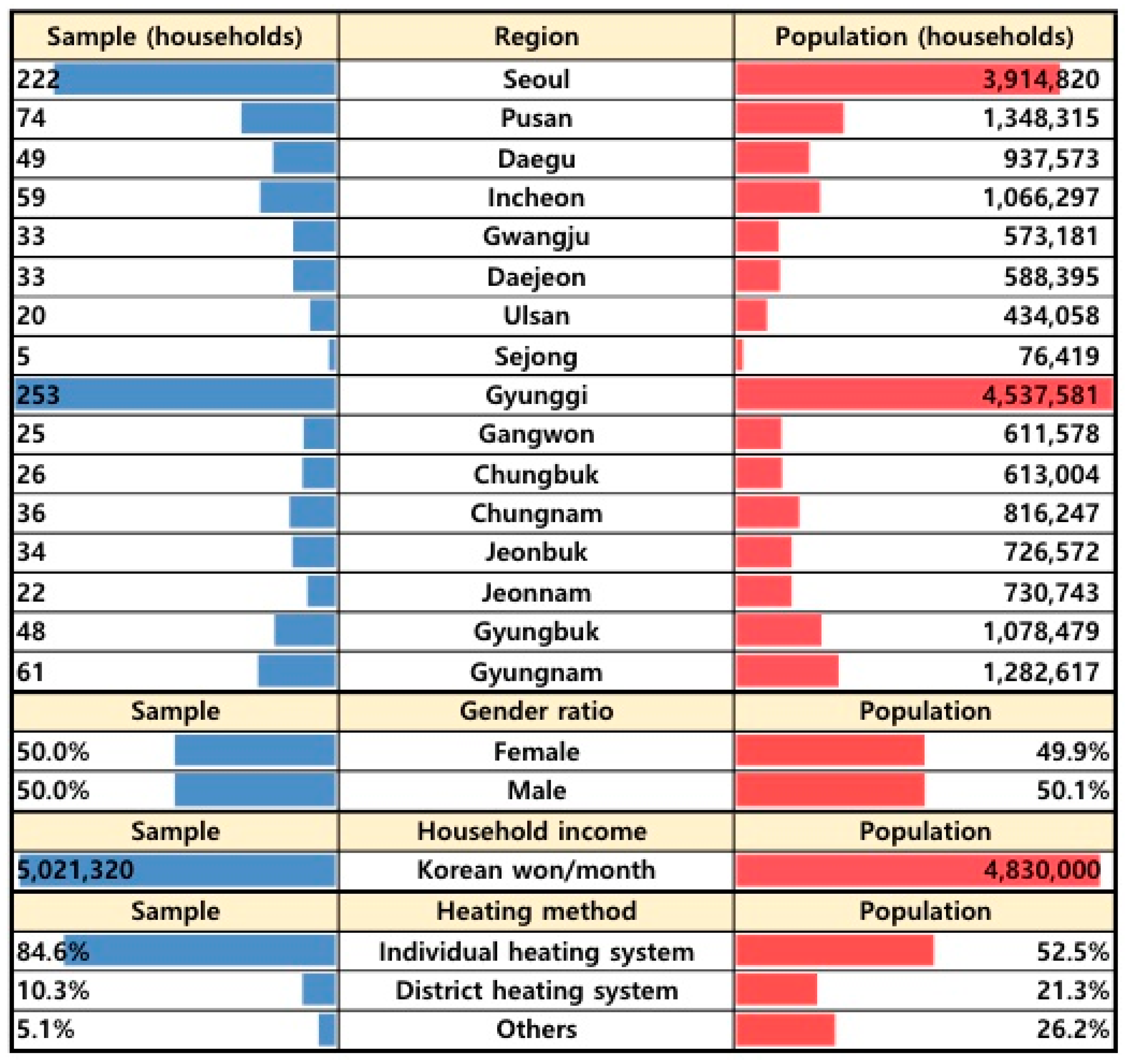
The survey for data collection was conducted in October 2019. The data for RCG use targets 2018. The authors tried to ensure the representativeness of the sample by conducting sampling based on the census data gathered in 2015 by Statistics Korea. In this regard, a comparison of the characteristics of the sample with those of the population is shown in Figure 1. It can be seen that there is not much difference between the values for the sample and those for the population.

As explained above, 114 out of 1000 households were non-consumers of RCG. The remaining 886 households used CG for cooking. Of these, 776 households also used CG for heating. Therefore, the number of households using CG only for cooking was 110. All households answered the questions about four hypothetical price changes without much difficulty. However, since some households did not keep their CG bill, information on CG usage and charges in 2018 was not obtained. In this case, the missing RP data for CG demand and price were replaced with the average value of the data for the responded households.

Table 1. Description of variables in the model.

Variables	Definitions	Minimum	Maximum	Skewness	Kurtosis	Median	First Quartile	Third Quartile	Mean	Standard Deviation	Expected Sign
RCG	Household consumption of residential city gas (RCG) per month (unit: m3)	2.40	333.00	1.10	2.91	55.00	33.00	74.00	57.33	34.47
P	Price of RCG (unit: KRW per m3)	88.24	2666.67	0.95	0.47	1028.57	875.00	1333.33	1132.56	340.95	(−)
Y	Household income per month (unit: KWR 1 million = USD 870)	1.00	20.00	1.23	3.91	4.80	3.50	6.00	5.02	2.15	(+)
F	Number of members in the respondent household	1.00	7.00	−0.27	−0.19	4.00	2.00	4.00	3.30	1.11	(+)
D	Whether the respondent uses RCG only for cooking (0 = no; 1 = yes)	0.00	1.00	−2.28	3.20	1.00	1.00	1.00	0.88	0.33	(−)
H	Whether the heating method of the household is an individual heating system (0 = no; 1 = yes)	0.00	1.00	−2.30	3.27	1.00	1.00	1.00	0.87	0.33	(+)
M	Whether the respondent resides in the Seoul Metropolitan area (0 = no; 1 = yes)	0.00	1.00	−0.14	−1.98	1.00	0.00	1.00	0.53	0.50	(?)

contains information on the definition, mean, and standard deviation of each variable used for the estimation of Equation (1). The RCG is defined as the average monthly CG usage during 2018. A total of six variables are considered in the list of independent variables, and these variables were selectively applied when estimating Equation (1). The first three variables were used by taking natural logarithms because they were continuous variables with positive values. As the next three variables were dummy variables, their original values were used. $P$, $Y$, and $F$ denote the average price of CG per m³, the average monthly income of respondent households, and the total number of members of respondent households, respectively. In addition, $D$, $H$, and $M$ indicate whether respondents’ households use CG only for cooking, whether respondents’ households use an individual heating system, and whether the respondent lives in the Seoul Metropolitan area.

3.2. Results

Table 2. Estimation results using least squares method.

Variables 1	Model 1	Model 2	Model 3	Model 4	Model 5	Model 6
Constant	8.194 * (27.04)	7.388 * (40.57)	7.271 * (37.22)	6.742 * (33.35)	7.424 * (40.74)	7.316 * (37.39)
$\ln P$	−0.676 * (−17.85)	−0.567 * (−25.25)	−0.566 * (−25.18)	−0.576 * (−24.52)	−0.572 * (−25.44)	−0.570 * (−25.36)
$\ln Y$	0.058 * (2.31)	0.035 * (2.07)	0.035 * (2.07)	0.199 * (12.83)	0.038 * (2.23)	0.038 * (2.23)
$\ln F$		0.359 * (20.00)	0.358 * (19.97)		0.361 * (20.13)	0.361 * (20.11)
D		−1.764 * (−88.64)	−1.660 * (−25.41)	−1.626 * (−23.83)	−1.745 * (−84.32)	−1.650 * (−25.25)
H			0.109 # (1.66)	0.122 # (1.79)		0.100 (1.52)
M				−0.033 * (−2.32)	−0.045 * (−3.30)	−0.044 * (−3.23)
F-values	161.30 *	2278.22 *	1823.84 *	1602.88 *	1828.82 *	1524.85 *
(p-values)	(0.000)	(0.000)	(0.000)	(0.000)	(0.000)	(0.000)
Adjusted-R2	0.068	0.673	0.673	0.644	0.674	0.674
Standard error of regression	0.7319	0.4335	0.4334	0.4523	0.4330	0.4330
Akaike information criterion	4904.9	2585.8	2585.4	2773.9	2581.4	2581.2
RMS%E 2	32.131	13.905	13.899	14.421	13.862	13.857
Sample size	4430	4430	4430	4430	4430	4430

¹ Explained in Table 1. ² RMS%E denotes the root mean square percent error. * and ^# denote statistical significance at the 5% and 10% levels, respectively. t-values are given in parentheses below the estimates.

contains the results based on the LS estimation method. A total of six models were set up where the selection of independent variables was different. The p-values corresponding to the F-value for all models are less than 0.01. Thus, all models are statistically significant. To select the appropriate one among these six models, a total of three pieces of information are used: adjusted-R², standard errors of regression (SER), and Akaike information criterion (AIC). In general, a larger adjusted-R² is preferred, and a smaller SER and AIC. In addition, to comparing the predictive power among models, the root mean square percent error (RMS%E) is estimated for all models. The model with this smallest value can be considered the model with the highest predictive power.

Interestingly, Model 6 has the largest adjusted-R², the smallest SER, the smallest AIC, and the smallest RMS%E. The price elasticity of demand was obtained as −0.570, securing statistical significance. Since its absolute value is less than 1, it can be seen that demand is inelastic in relation to price change. The income elasticity was found to be 0.038, holding statistical significance. Thus, demand is also inelastic in respect of income change.

Table 3. Estimation results using least absolute deviations method.

Variables 1	Model 1	Model 2	Model 3	Model 4	Model 5	Model 6
Constant	7.631 * (35.31)	6.821 * (47.74)	6.644 * (43.37)	6.511 * (41.08)	6.787 * (47.46)	6.636 * (43.26)
$\ln P$	−0.648 * (−24.00)	−0.509 * (−28.87)	−0.509 * (−28.91)	−0.518 * (−28.14)	−0.510 * (−28.94)	−0.512 * (−29.02)
$\ln Y$	0.144 * (8.09)	0.062 * (4.71)	0.063 * (4.73)	0.163 * (13.40)	0.071 * (5.32)	0.069 * (5.24)
$\ln F$		0.359 * (25.47)	0.357 * (25.38)		0.370 * (26.32)	0.366 * (26.01)
D		−1.807 * (−115.75)	−1.626 * (−31.73)	−1.598 * (−29.87)	−1.798 * (−110.77)	−1.623 * (−31.67)
H			0.182 * (3.54)	0.179 * (3.34)		0.175 (3.40)
M				−0.015 (−1.32)	−0.036 * (−3.38)	−0.037 * (−3.48)
F-values	258,565.4 *	575,844.1 *	576,797.9 *	532,772.7 *	576,797.2 *	578,049.2 *
(p-values)	(0.000)	(0.000)	(0.000)	(0.000)	(0.000)	(0.000)
Adjusted-R2	0.065	0.672	0.672	0.643	0.672	0.673
Standard error of regression	0.7503	0.4342	0.4341	0.4533	0.4340	0.4338
Akaike information criterion	4624.1	2728.3	2725.9	2913.1	2724.8	2722.2
RMS%E 2	34.643	13.869	13.888	14.560	13.818	13.842
Sample size	4430	4430	4430	4430	4430	4430

¹ Explained in Table 1. ² RMS%E denotes the root mean square percent error. * denotes statistical significance at the 5%. t-values are given in parentheses below the estimates.

reports the results from estimating the RCG demand function using the LAD estimation method. The Wald statistics are computed under the null hypothesis that all coefficient estimates are zero. Since the p-values corresponding to the Wald statistics are less than 0.01 in all six models, all models guarantee statistical significance. The model with the largest adjusted-R², the smallest SER, the smallest AIC, and the smallest RMS%E was Model 6. The price and income elasticities of demand were revealed as –0.512 and 0.069, respectively, and both had statistical significance. The qualitative interpretation of the magnitude of these two elasticities is not different from the estimation results using the LS method.

The two important hypotheses formulated in this study are as follows. The first hypothesis is that the price elasticity of RCG demand is less than zero. This hypothesis aims to confirm whether the law of demand presented in microeconomics is established. The law of demand means that the demand for a particular good is inversely proportional to the price of that good. If the law of demand is secured, the price elasticity must be negative. A one-sided t-test may be applied to determining whether the hypothesis is satisfied. When the test statistic is T, the rejection area at the significance level of 5% is T > 1.645. Since the test statistic of Model 6 in Table 2 is calculated as −25.36 and is not included in the reject area, the hypothesis cannot be rejected. Therefore, at a significance level of 5%, the RCG satisfies the law of demand. Lowering the significance level to 1% or raising it to 10% does not change this finding.

The second hypothesis is that the income elasticity of demand is greater than zero. According to microeconomics, for a normal good, not an inferior good, the income elasticity of the demand for it must be greater than zero. In other words, the demand for a normal good must increase as income increases. RCG is clearly a normal good. Thus, the hypothesis should not be rejected. Similarly, a one-sided t-test applies to determining whether the hypothesis is met or not. When the test statistic is T, the rejection area at the significance level of 5% is T < −1.645. Because the test statistic of Model 6 in Table 2 is computed as 2.23 and is not contained in the reject area, the hypothesis is not rejected. At the significance level of 5%, RCG can be said to be a normal good. Even if the significance level is lowered to 1% or raised to 10%, this qualitative conclusion remains the same.

4. Discussion

In this section, the results presented above will be discussed from three angles. First, we consider which of the estimation results should be selected from those using the LS method and those using the LAD method. Since the dependent variables are the same regardless of the estimation method, the results with smaller SER and smaller AIC can be adopted. As Model 6 was adopted in both Table 2 and Table 3, the estimation results of Model 6 are compared. Using the LS method, the SER and AIC are 0.4330 and 2581.2, respectively. Using the LAD method, they are 0.4338 and 2722.2, respectively. The former values are smaller than the latter. Therefore, subsequent discussions in this study are based on the results of applying the LS estimation method to Model 6.

Second, policy implications deriving from the estimated demand function can be discussed. As mentioned earlier, the price elasticity of demand has a negative value of −0.570. This means that RCG satisfies the law of demand presented in microeconomics. In addition, its absolute value is less than 1. Therefore, RCG demand is inelastic in relation to price change. This is a good representation of the demand characteristics of RCG—it is difficult to reduce cooking or heating significantly even if the price of RCG rises significantly, and it is difficult to increase cooking or heating significantly even if the price falls significantly. Using this elasticity value, it is possible to predict changes in demand when raising or lowering the price of RCG in the future.

Because the income elasticity of demand is 0.038, which is positive and statistically significant, RCG is clearly a normal good. However, the value is less than 0.1. Although the estimated income elasticity has statistical significance, its actual value is quite low. This means that even if income increases or decreases a lot, demand for RCG will only increase or decrease a little. Therefore, demand for RCG will increase as income increases, but the scope of the increase is tiny. It can be predicted that even if income increases with economic growth in the future, the increase in demand for RCG will be limited.

Third, it is possible to use the estimated demand function and assess the benefits of using RCG. From a microeconomics point of view, the benefits arising from the consumption of a particular good are the flipside of the demand function for that good. This area is divided into consumer surplus and consumer expenditure. Consumer expenditure is easily determined, while consumer surplus is generally not easily obtained. This is because consumer surplus can be measured only when there is a price at which demand becomes zero and the level of the price is identified. If the price is difficult to find, it is difficult to determine the consumer surplus quantitatively. Accordingly, Alexander et al. [31] developed and presented a formula for calculating the consumer surplus, $CS$, as follows.

$$CS=-\frac{P_0{Q}_0}{2\mu }$$

(2)

where $P_0$ and $Q_0$ refer to the current price and consumption, respectively, and $\mu$ is the price elasticity of demand. Therefore, the numerator on the right side of equation (2) is consumer expenditure. Information on $\mu$ is required to compute Equation (2). As mentioned earlier, the price elasticity was obtained as –0.570. The consumption benefits of RCG can be derived as follows:

$$P_0{Q}_0+CS=P_0{Q}_0-\frac{P_0{Q}_0}{2\mu }=1.877P_0{Q}_0$$

(3)

Substituting the averages of the consumption variable (RCG) and the price variable (P) presented in Table 1 into $P_0$ and $Q_0$ in Equation (3), we arrive at the consumption benefit of RCG in terms of the average household. Dividing this value by $Q_0$ again, the consumption benefit per unit of RCG is derived as KRW 2125.82 per m³. This value is useful for computing the economic benefits arising from enforcing a new RCG supply project: in other words, the economic benefit of carrying out the project to supply 1 million m³ of RCG every year amounts to around KRW 2.1 billion.

5. Conclusions

Both the government and the 34 CG operators are seeking information on the demand function for RCG. However, in obtaining the demand function, researchers face two complications: (a) difficulty obtaining RCG transaction data; and (b) the possibility of distortion of market prices. To overcome these complications, this study attempted to employ the PSM technique to estimate the RCG demand function. To this end, the average price was derived by asking each household about its current RCG consumption and expenditure, and SP data were collected by asking four times about the demand change for the hypothetical price change alternative from this average price. Therefore, one set RP data and four sets of SP data were collected for each household.

In short, 4430 observations on price and demand for RCG from 886 households nationwide were analyzed. Six demand function models were established and estimated. The LAD estimation method and the LS estimation method were applied. The price and income elasticities from the adopted demand function were –0.570 and 0.038, respectively, and showed statistical significance. Since RCG has the property of being an essential good, the absolute value of price elasticity was less than 1.0. Although RCG is a normal good, demand responds to income change quite inelastically. These findings showed the essential nature of RCG.

The purpose of this study was to estimate the RCG demand function in South Korea. The authors think that this estimation has some significance not only in terms of research for scientific knowledge but also in terms of deriving important implications. This study made two contributions in terms of research. First, the PSM technique to overcome some difficulties in securing data for estimating the RCG demand function was successfully applied. The PSM technique was mainly applied in the tourism field, and it was confirmed in this study that it could be useful in dealing with energy demand. Second, the authors attempted to derive the final demand function by attempting various efforts to apply two estimation methods and various criteria for choosing a proper model. More specifically, not only the LS estimation method but also the LAD estimation method were used, and a total of four criteria such as adjusted-R², SER, AIC, and RMS%E were employed.

Furthermore, this study has three significances in terms of policy. First, the price elasticity of RCG demand was found to be −0.570, securing statistical significance. NG tends to have greater international price volatility than other energies. Since NG must be secured stably for a stable supply of RCG, the government is paying special attention to the need for NG terminals, tanks, and pipelines. Therefore, in a situation where the government is essentially demanding information on the price elasticity, this study disclosed it. Second, the income elasticity of RCG demand was statistically significantly observed as 0.038. Although this value was not large, it was significantly greater than zero. In other words, it was suggested that RCG demand will increase at a relatively modest rate according to future economic growth. Third, the obtained price elasticity information was used to estimate the economic benefit arising from consuming RCG, and the benefit was 1.877 times the price. In South Korea, a new project of supplying RCG continues to be proposed and carried out as the number of households that want to be supplied with RCG but have not yet been supplied reaches 2 to 3 million. Therefore, information about the consumption benefit can be used to compute the economic benefits in assessing the economic feasibility of a new RCG supply project.

This study is significant in applying the PSM technique for the first time in the literature to estimate the demand function of RCG. Nevertheless, future research tasks emerge. The authors hope that five major tasks will follow. First, this study only deals with data on South Korea, but if data on other countries can be obtained and dealt with, a comparative study can be carried out. The comparison may present interesting implications. Second, in this study, a total of six variables, including price and income, were considered in addition to the constant term as independent variables of the demand function, but more variables need to be considered, as there are various factors that may affect demand. It would be better to estimate the demand function while comprehensively reflecting various factors and then derive price and income elasticities.

Third, if regional surveys are conducted and demand functions of RCG are obtained by region, regionally differentiated implications can be derived. In particular, since South Korea has adopted a regional monopoly system in RCG supply, the estimation of the regional demand function of RCG can be quite significant. To this end, efforts must be made to raise the number of the entire observations by securing a sufficient survey budget. Fourth, a study may be conducted to estimate the demand function of electricity or residential heat-based district heating system that is competitive with RCG. A comparison of each result can lead to meaningful implications.

Fifth, it is necessary to estimate the demand function by combining the consumer relationship management data of RCG operators and information on variables collected through a survey using the consumer contact information. In other words, it is necessary to compare the demand function based on the revealed preference data and the demand function based on the stated preference dealt with in this study. If there is no significant difference between the two, it can be confirmed that the stated preference data collected through the PSM technique are also useful in obtaining the demand function. If there is a difference between the two, the cause of the difference can be explored.