1. Introduction
In the last years there has been a systematic action of enterprises to adopt policies that lead to a transition toward a low-carbon economy. Furthermore, the potential investors systematically seek to enclose in their portfolios more environmentally friendly investments. Their activities enhanced a new investment tool, the corporate green bonds. With simple words, these are corporate bonds that are committed exclusively to financing green projects (environmentally and climate-friendly projects). Renewable energy projects in Turkey, hydropower plants in Rampur in India and energy efficiency investments in Tunisia are some examples of successful green bond projects as mentioned by the World Bank green bonds impact report (World Bank, 2017) [
1]. In 2018, the issuance of green bonds was approximately 250 billion USD as estimated by Moody’s, which is expected to touch 1 trillion USD by 2021. Premium of green bonds is different than non- green bonds (Zerbib, 2019) [
2]. There are a variety of factors that affect the green premium such as environmental, social and economic factors (MacAskill et al., 2020) [
3]. The premium is different in the primary and secondary markets. For instance, in the case of the secondary market, green bonds offer up to 70% premium. However, in the case of the primary market, there is no evidence on the percentage of premium. These bonds are growing and evolving rapidly, incorporating changes in the socio-economic environment. Although a considerable number of recent studies highlight the growing interest in green bonds (for instance, Monk and Perkins, 2020 examine in detail the emergence and diffusion of green bonds), very little attention is given to the relationship with commodities (Nguyen et al., 2020, Naeem et al., 2021, Naeem et al., 2021) [
4,
5,
6].
To cover this research gap, in contrast to previous studies, we move to the persistent investigation of a long-term relationship between green bonds and commodities. Furthermore, we include a significantly higher number of commodities and observations. However, for first time in relative research activity we adopt VaR (value at risk) based copulas to describe the asymmetric risk spillover between green bonds and commodities by considering the asymmetric tail distribution. Following the literature on risk spillover between green bonds and the financial market, we further investigate how uncertainty from the commodity market results in risk spillover of green bonds. During COVID-19, the volatility of financial markets increased (Li, 2016) [
7]. Our analysis will open new pathways both for potential corporate green bonds investors (e.g., portfolio design, risk management) and makers of environmental policy (e.g., acceleration of improvement of environmental footprint by enterprises).
We contribute to the emerging strand of studies that examine the causality and dependence between financial and green bond markets during the outbreak of COVID-19 pandemic. In particular, our study has many contributions. First, we include a significantly higher number of commodities and observations. Further, to the best of our knowledge, no other study has applied VaR-based copulas to investigate the dependency structure among green bonds and commodities. We investigated the predictive power of the green bond market on the commodity market during the outbreak of the COVID-19 pandemic. Additionally, we have explained the relationship between green bonds and commodities in the long run, which covers the COVID-19 pandemic period. The study will be beneficial to portfolio managers, who can make use of green bonds to diversify the risk of the commodity market.
We document several interesting findings. First, extreme price movements have no impact on volatility of WTI and agriculture commodities. Second, natural gas and copper exhibit safe heaven properties when paired with green bonds. Third, spillover effect is lowest in the case of energy commodities. Gold has the strongest positive connection with green bonds. Further, there is an insignificant relationship between green bonds and commodities as against the findings of Naeem et al. (2021) and Naeem et al. (2021) [
4,
5]. Additionally, perishable commodities other than lead are transmitting risk to non-perishable commodities. Green bonds have emerged as a net receiver of shocks from the commodity market.
The remainder of the paper is organized as follows.
Section 2 provides a detailed review of the relative literature.
Section 3 introduces the data and the methodological framework.
Section 4 presents the empirical findings, together with a discussion of the results and policy implications. Finally,
Section 5 concludes the paper.
2. Literature Review
First, it deserves mention that a significant part of the relative literature has explored the connectedness of commodities with the energy market (see, for instance, Albulescu et al., 2020; Balli et al., 2019; Mensi et al., 2017; Dutta et al., 2018) [
8,
9,
10,
11].
More precisely, López Cabrera & Schulz (2016) [
12] give emphasis to the volatility spillover between energy and agriculture commodities. The authors calculate the hedging ratios as well using copulas. The study highlighted the transformation in the relationship between energy and agriculture commodities because of the change in consumption pattern of biofuels. Dutta et al. (2018) [
10] points out that positive changes in the crude oil prices have a more severe impact on selected metals as compared to negative changes. Similarly, Mensi et al. (2017) [
11] examined the correlation among commodity indices and found a time-varying asymmetric tail dependence between the pair of cereals as well as between oil, wheat, and corn. Their study highlights the benefits of oil and agriculture commodities as a risk hedging tool. Another prominent study is from Balli et al. (2019) [
9]. The authors used structural VaR to study the impact of risk spillover on daily prices of 22 commodities. They found that the commodities exhibited strong connectedness during the global financial crisis (GFC). Then, Albulescu et al. (2020) [
8] investigated the interconnectedness among the commodity market viz agriculture, metals and energy using copula analysis. Their study also revealed that, during the financial crisis, energy is not a good tool of hedging risk as compared to other commodities.
Despite the short period of development of corporate green bonds, an increasing number of studies emphasize the explanation of their features and performance. For instance, Flammer (2020) [
13] states that, apart from environmental performance, these bonds have financial and ESG implications as well. Supporting this claim, Bofinger et al. (2022) [
14] stated that a firm can enhance its valuation by fulfilling its ESG criteria as a response to positive market sentiment. Earlier, Zerbib (2017) [
15] exhibited that demand of green bonds is comparatively low with respect to conventional bonds. His study also revealed that the rating affects the premium of green bonds. On the same wavelength, Baker et al. (2018) [
16] show that green bonds carry higher premium as compared to other conventional bonds. The premium is even higher when these bonds are certified. Tang & Zhang (2020) [
17] examine how the shareholders are benefitted by the issuance of green bonds. However, in terms of financial performance the return on green bonds was lower as compared to conventional bonds. Moreover, the issuance of green bonds attracts the interest of media which in turn enhances the image of the issuing firm. Finally, Flammer (2021) [
18] shows that investors respond positively to the issuance announcement. This response is stronger for first-time issuers and bonds certified by third parties. Her research differs from the previous research of Tang and Zhang (2020) [
17] because she examines how firm-level outcomes evolve following the issuance of green bonds. Furthermore, her study implies that the issuance of green bonds can help firms to fulfil its social responsibilities. Alonso-Conde and Rojo-Suárez (2020) [
19] have analysed the profitability and solvency of green projects. The study found that green bonds are beneficial for issuers too, apart from fetching higher returns than conventional bonds. In addition, the issuance of green bonds results in an increase in the IRR for shareholders in the energy project financing.
Another significant strand of literature emphasizes the relationship of green bonds with other financial markets. Firstly, the researchers focus on the comparison and relationship with conventional bonds. Hachenberg & Schiereck (2018) [
20] found a close association between them while they revealed that pricing of green bonds is significantly different from non-green bonds. Later, Reboredo et al. (2020) [
21] reported the diversification benefit of green bonds in response to the energy market. Their study also revealed that green bonds are more popular in the UK and US markets. Further, Saeed et al. (2020) [
22] examined the risk and return spillover between clean and dirty energy using mean-based connectedness measures. They showed that green bonds are not affected by the risk-return spillover effects. This feature makes them attractive for diversification unlike conventional energy assets. Afterwards, Nguyen et al. (2021) [
6] found that the interdependency among green bonds and other financial markets increased spontaneously post-GFC. However, the connectedness among green bonds and stocks and green bonds and commodities is weak. Similarly, Liu et al. (2021) [
7] stated that the green bonds market is not completely developed. Naeem et al. (2021) [
5] and Naeem et al. (2021) [
4] have explained the co-movement between green bonds and commodities and found that the spillover among green bonds and commodities is strong during financial crises.
The most recent studies examine the tailed dependency of the green bond market with other asset classes. For instance, Liu et al. (2021) [
23] explored the dependency between green bonds and clean energy markets by using CoVaR. Tailed dependency was found between green bonds and clean energy implying that both markets together experience an up and down trend. They result in a positive link between green bonds and clean energy. Reboredo (2018) [
24] applied copulas to reveal that pricing of green bonds is not clearly affected by the energy and stock returns.
The previous studies use a diverse range of econometric methods to explain the relationship between green bonds and clean energy (Liu, et al., 2021; Zerbib,2016) [
7,
25], cryptocurrencies and oil (Yin, et al., 2021; Gronwald,2019; Okorie, & Lin,2020) [
26,
27,
28], safe haven properties of green bonds (Tang, & Zhang, 2020; Zerbib, 2016) [
17,
25] and commodities connectedness (Albulescu et al., 2020; Balli et al., 2019; Mensi et al., 2017 and Vacha & Barunik, 2012) [
8,
9,
11,
29]. In a prominent research study, Nguyen et al. (2021) [
6] explain the relationship among green bonds and various asset classes, namely conventional bonds, equity, and commodities. In addition, Naeem et al. (2021) [
4] exhibit the dependency between green bonds and commodities in the short term. One of the main contributions of our research with respect to these two papers concerns the persistent investigation of a long-term relationship between green bonds and commodities. Furthermore, we include a significantly higher number of commodities and observations. Additionally, we found an insignificant relationship between green bonds and commodities, both perishable and non-perishable (with select exception). In this context, for the first time in relative research activity we adopt VaR (value at risk) based copulas to capture the connectedness among green bonds and commodities.
3. Data Description and Methodology
In our study we explore the dependence between commodity futures markets and green bond returns based on daily data of ten Bloomberg Commodity Index commodities, which includes Western Texas Intermediate (WTI) crude oil, natural gas, heating oil, silver, gold, copper, lead, corn, wheat, and coffee. Therefore, we provide wide-ranging coverage of commodity markets by investigating three energy commodities, four metals, two base and three main agricultural commodities. The S&P Green Bond Index is used as a proxy for the green bond market. The data for the S&P Green Bond Index were obtained from the S&P Dow Jones Indices while those for commodities were obtained by a database of Bloomberg. The Western Texas Intermediate (WTI) crude oil is a scientific grade of crude oil, being sourced from Texas. It is a high-quality crude oil which can be easily refined. Heating oil, also known as fuel oil, is a petroleum product. Natural gas is a combination of gases in the atmosphere like methane, carbon dioxide and hydrogen sulfide. It is also referred to as fossil gas. Silver and copper are precious and industrial metals. Gold is a rare precious metal which is used for financing, investing and jewelry. Lead is a non-perishable commodity, which is mainly used in batteries and ballast. Corn, coffee and wheat are perishable commodities used for agriculture consumption. The description of the data is provided from the following
Table 1.
The data sample of daily data spans the period between 30 March 2011 to 6 May 2021. The reason behind this time period solely rests on the fact that it comprised many turbulent events, such as the Crimea annexation (2014), Greek Debt Crisis (2015), BREXIT (2016) and COVID-19 (2020).
The contribution of our study is enhanced by the adoption of the copula theory within the framework of Patton (2009) [
30]. In this way, we study the dependency pattern among green bonds and commodities using conditional distribution. Patton (2009) [
30] has defined copulas as follows:
Let
, for r = 1, 2, …,
x be the random variables of
and
is a joint probability function of
, where ω is a support function of
and
(
=
).
is a copula function for each
ϵ
and
ϵ ω.
is unique if ;...; are all continuous. F is a conditional function with marginals , …….,.
F is an n-dimensional conditional distribution function with continuous marginals
,
…….,
and copula
, where
for any
in [0, 1]
and Zϵ ω;
Let R be the maximum loss incurred due to the losses that are caused by two series R1 and R2, so that R = R1 + R2. The total risk R is affected by the dependence between the risk of those two series.
There exists a copula function
:[0, 1]
2 ∈ [0, 1], which depends on parameter value θ, for a given (
R1,
R2) a random vector of risk components with
1 (r
1) = Q(
R1 =
r1) and
2 (
r2) = Q(
R2 =
r2) their respective continuous distribution functions
while
=
H1 (
) and
=
H2 (
) are the values of two random variables
that are uniformly distributed on the interval (0, 1).
Estimation of one or more parameters is necessary to determine the fitness of the copula, which is estimated with the help of pseudo-maximum likelihood as follows:
Finally, value at risk (VaR) for each copula is estimated within the framework of Mendes, 2005 [
31] using the following step
where
denotes the desired level of confidence.
4. Empirical Findings and Discussion
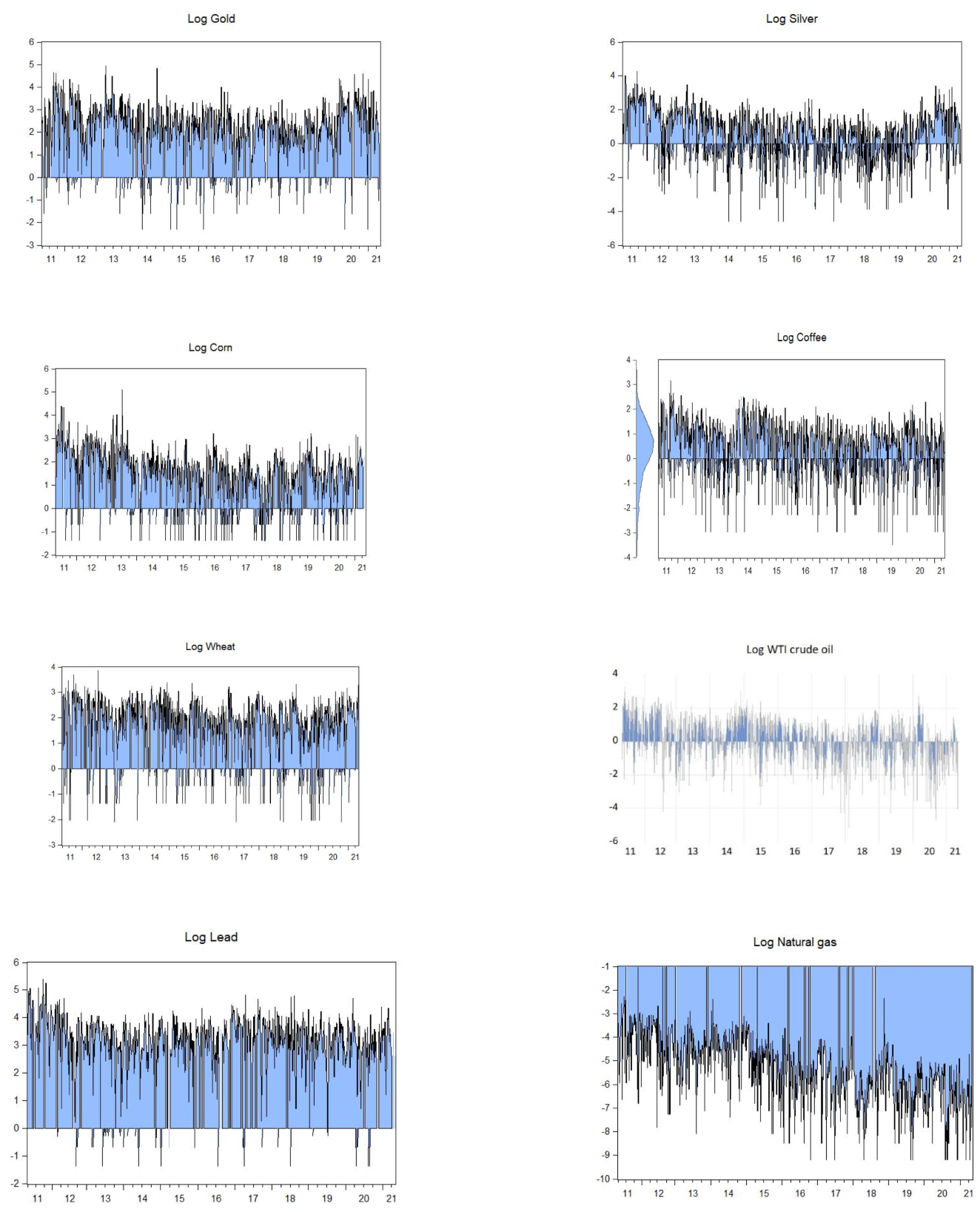
We begin our analysis with a simple illustration that shows the dynamics of logarithmic returns in the commodity market and green bonds (
Figure 1).
Clearly the commodity returns are especially volatile after 2020 with the novel coronavirus outbreak. The gold, silver and agriculture commodity returns display a similar volatility pattern, whereas the copper, lead and metals dynamics show no temporal pattern.
In continuation we provide a descriptive presentation of the data.
Table 2 summarizes the descriptive statistics on the commodities under consideration, and on the S&P Green Bond Index.
Here standard deviation is used as a measure of volatility. The descriptive statistics demonstrate that silver is considerably less volatile than corn and wheat. Lead was found to be the largest receiver of up to four times higher returns than that of other commodities. The average returns are highest for heating oil and lowest for the S&P Green Bond Index. Positive values for skewness are common for all commodities except coffee and wheat. All returns exhibit excess kurtosis.
In the next step we provide Spearman’s rho and Kendall’s tau correlation between green bonds and commodities considering the non-normality of the variables.
We have a positive correlation between green bonds and lead, silver, copper, gold, and wheat. This implies that these markets experience upward and downward trends together. However, the correlation is negative in the case of WTI crude oil, heating oil, natural gas, corn, and coffee, implying that markets move in opposite directions. According to Spearman’s rho and Kendall’s tau, gold and green bonds have the strongest positive connection. The highest negative value is detected between green bonds and heating oil holds.
Correlation is not sufficient to offer a clear direction about the dependency between green bonds and commodities. For this reason, we adopt copulas to capture the connectedness between green bonds and commodities.
Table 3 shows the lower tail and upper tail dependency parameters of various copulas.
Clayton shows the asymmetric dependency at lower tail and Gumbel captures a respective asymmetric dependency at upper tail. According to Liu et al. (2017a) [
7], different copulas exhibit different properties. For instance, Student’s t copula can capture the symmetric tail dependence while Gaussian copulas fail to describe the tail dependence; since most asset classes globally aren’t strictly Gaussian, rather they follow log-normal distribution. Frank copula is used when there exists a greater dependency at both the tails rather than the median.
In
Table 4 we show the AIC and BIC (penalties for reducing errors) values based on the dependency parameters and log-likelihood of Gaussian copulas(α), Student’s t copulas(β), Gumbel copulas(λ), Clayton copulas(γ), and Frank copulas (δ) to explain the dependency among green bonds and various commodities, namely metals, agriculture, and energy.
AIC and BIC values are used as a basis for selecting the best lag combination for each marginal model. Various copulas for each green bonds and commodity pair are compared on the values log-likelihood, BIC, and AIC. For heating oil and coffee, the AIC and BIC values were highest for the Clayton copula(γ) and AIC and BIC values were highest for the Gaussian copula(α) in the case of lead and copper. On the other hand, in the case of WTI crude oil, silver, gold, and wheat, the AIC and BIC receive maximum values for the Frank copula(δ) and AIC and BIC values were maximum for the Gumbel copula(λ) in case of corn and natural gas. AIC and BIC values were minimum for the Student’ t copulas(β) in case of all the commodities.
In
Table 5 we provide the value at risk (VaR) at different percentiles for each copula. We show the tailed dependency of maximum risk between green bonds and each commodity. We estimate VaR as the information criteria log-likelihood, BIC and AIC are not sufficient to lead a precise conclusion to which copula is the best fit to the data.
Table 6, shows the VaR values of each commodities against green bonds at 90th, 95th and 99th percentile. As regards lead, the VaR is minimum for the Gumbel copula. In the case of heating oil and natural gas, Student’s t copula has the minimum value at the 90th percentile, while the Frank copulas hold the minimum value at the 95th and 99th percentiles. For silver and gold, the Gumbel copula has the minimum value at the 90th, 95th, and 99th percentiles. In case of copper and wheat, VaR is minimum for Gumbel copulas at 90 percentiles, while the Frank copula holds the minimum value at the 95th and 99th percentiles. VaR value was at minimum for the Frank copula at the 90th, 95th, and 99th percentiles in the case of corn. In the case of coffee, the Clayton copula holds the minimum value at the 90th percentile and at the 95th and 99th percentile the Frank copula has the minimum value. VaR receives the lowest value in case of natural gas and copper when paired with green bonds. On the other hand, lead followed by gold obtains the maximum value of VaR. Therefore, risk becomes minimum for a portfolio with a fusion of green bonds, natural gas, and copper. Contrary to this, lead, gold and agriculture commodities are more volatile when paired with green bonds as their joint probability of VaR is higher.
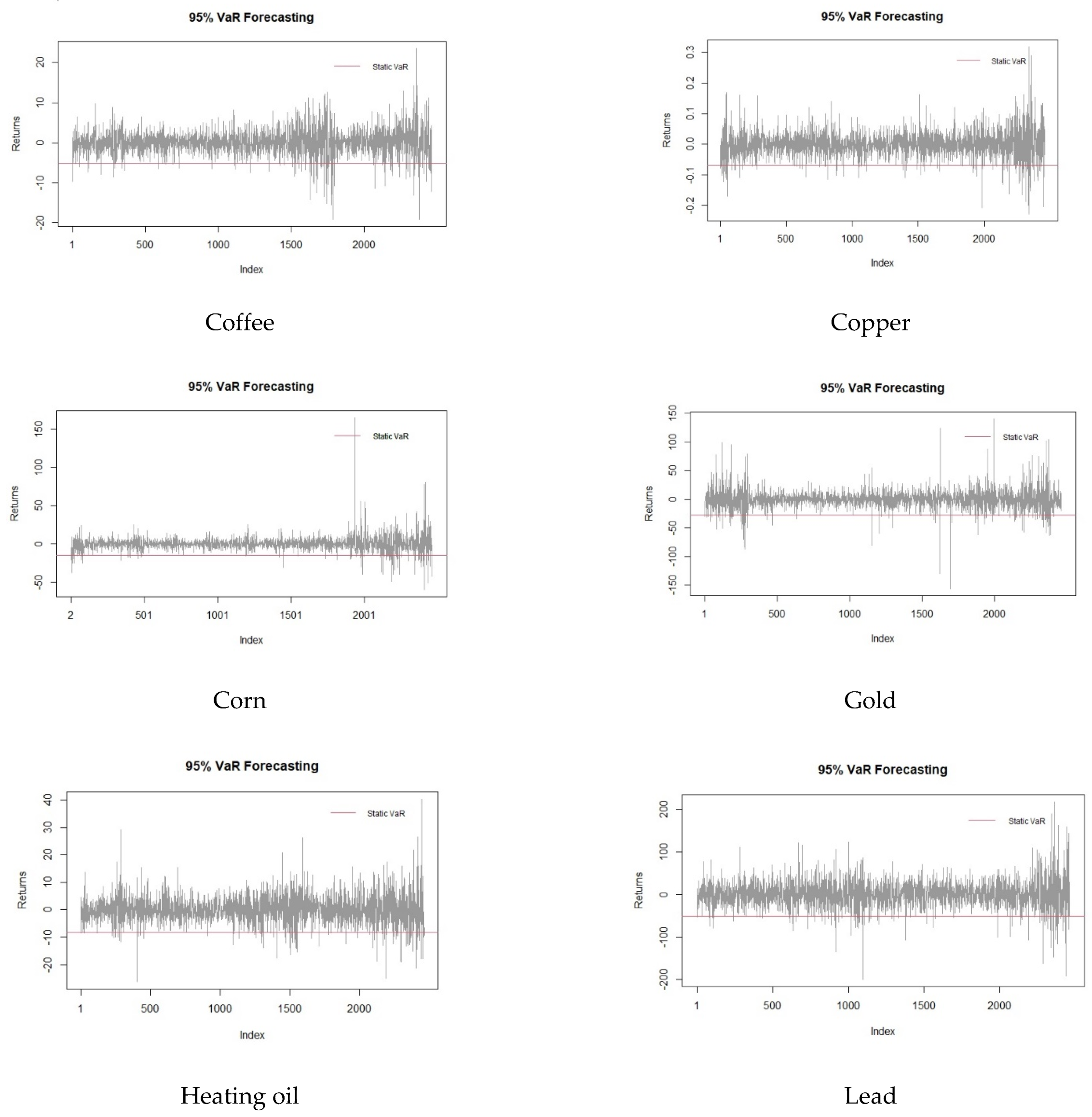
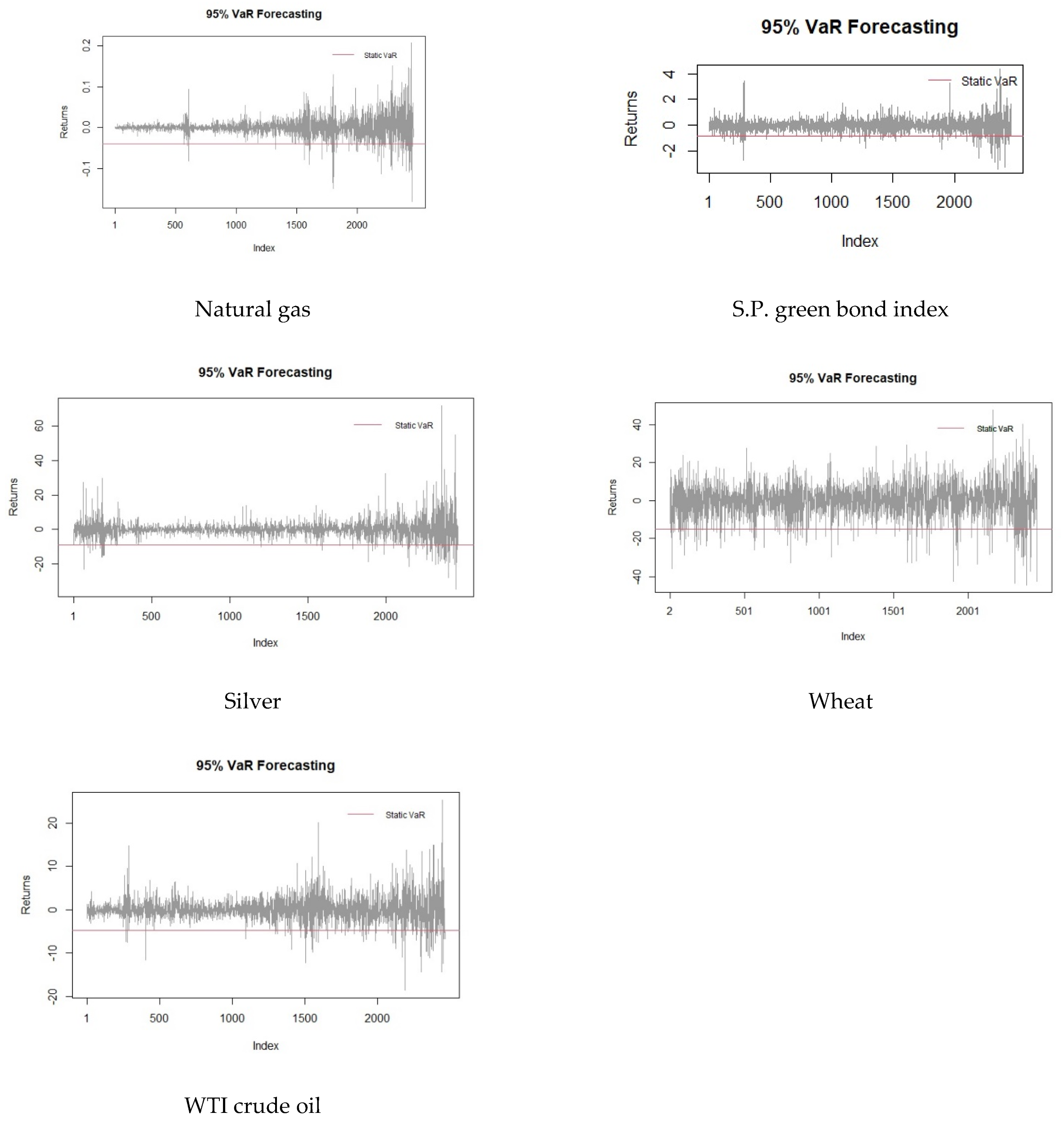
Figure 2 shows at value at risk (VaR) for the selected commodities and green bonds at 95% forecasting. The red line is VaR at a level of 95%. All the points below the red line are at risk at 95%. We can observe that fluctuation increases at the extreme right end for all the commodities and green bonds.
Figure 2 clearly shows gold to be least risky commodity, followed by silver and corn. WTI crude oil is the riskiest commodity, followed by wheat. The graph of lead is similar to heating oil.
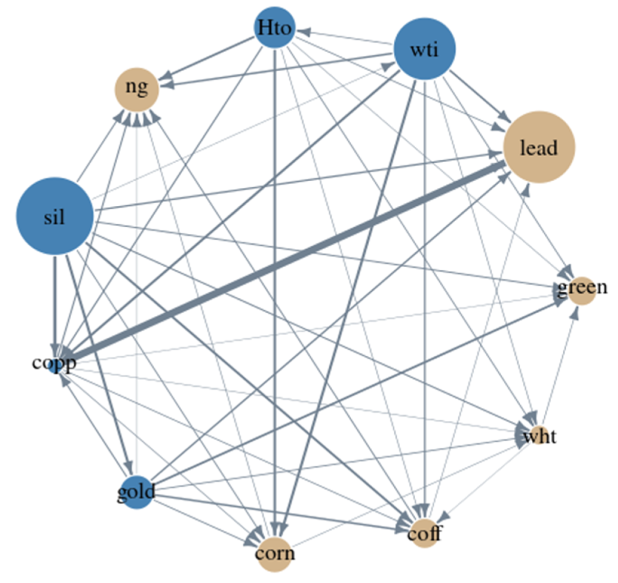
Figure 3 shows the network plot of green bonds and commodities. The figure clearly shows that the connectedness among various commodities and green bonds is very mild. Commodities with yellow nodes depict the effect of the net receiver of shocks, while commodities with blue nodes represent the effect of the net transmitter of shocks. The edges show the connectedness among the commodities and green bonds. Most of the commodities emerged as net receivers of shocks, which comprises of lead, green bonds, coffee, corn, wheat and natural gas, while silver, heating oil, WTI crude oil, copper and gold emerged as net transmitters of shocks. Further, lead and silver emerged as net receiver and transmitter of shocks, respectively. The connectedness was strongest between lead and copper. Lead receives shocks from WTI crude oil, heating oil, silver, gold, and coffee. Green bonds receive shocks from WTI crude oil, heating oil, silver, copper, gold, and wheat. Wheat receives shocks from WTI crude oil, heating oil, silver, copper, gold, and corn, while transmitting shocks to coffee. Coffee receives shocks from WTI crude oil, heating oil, natural gas, silver, copper, gold, and wheat, while transmitting shocks to lead. Corn receives shocks from heating oil, WTI crude oil, silver, copper, and gold, while transmitting shocks to natural gas. Natural gas receives shocks from silver, copper, gold, corn, coffee, WTI crude oil, and heating oil. On the other hand, gold is transmitting shocks to copper, lead, green bonds, wheat, coffee, and corn, while receiving shocks from silver. Copper is transmitting shocks to corn, coffee, natural gas, wheat and green bonds, while receiving shocks from gold, silver, heating oil and WTI crude oil. Heating oil is transmitting shocks to natural gas, copper, corn, coffee, wheat, green bonds, and lead, while receiving shocks from WTI crude oil. WTI crude oil is transmitting shocks to heating oil, natural gas, copper, corn, coffee, wheat, green bonds, and lead, while receiving shocks from silver. In other words, we can say that perishable commodities are receiving shocks from non-perishable commodities barring lead.
5. Concluding Remarks
In recent years, investors have systematically sought to enclose in their portfolios more environmentally friendly investments. Their activities enhanced a new investment tool, namely the corporate green bonds. These bonds are growing and evolving rapidly, incorporating changes in the socio-economic environment. However, studies regarding the relationship with commodities are still limited. To address this limitation, we adopt VaR (value at risk) based copulas to illustrate the asymmetric risk spillover between green bonds and commodities by considering the asymmetric tail distribution. Following the literature on risk spillover between the green bonds and the financial market, we further investigate how uncertainty from the commodity market results in risk spillover of green bonds.
We found an asymmetric spillover effect among commodities (with varying degrees) and green bonds. This dependency structure among various commodities was also found to be very weak. In other words, we can say that green bonds can be used to hedge the risk of commodities to a certain extent. The results indicated metals to be risker in comparison to agriculture and energy commodities. The outcome of the study can aid policymakers and investors to frame sound investment decisions. It can be beneficial to investors who mostly rely on banks to hedge their portfolio risk by fusing green bonds with commodities. As the study includes a large number of commodities, it can aid investors to explore the impingement of these commodities on green bonds for portfolios. The results of the study can be helpful for issuers of green bonds while framing policy decisions. Future research might examine the co-movement of other financial assets on green bonds or the impact of green bonds on the subcategorization of commodities viz energy, metals, and agriculture.
Our study provides various critical findings. First, we identify the asymmetric properties of different copulas of selected commodities. Second, by employing VaR quantiles for each copula, we estimate the dynamic risk spillover (very mild) between green bonds and the commodity market. The results from the network plot reveal an insignificant risk spillover effect from non-perishable commodities (barring lead) market uncertainty to natural gas, corn, copper, wheat, and green bonds. Therefore, we can have our third finding. Non-perishable commodities are transmitting risk to perishable commodities (barring lead). In contrast to the study of Naeem et al. (2021) [
5], risk spillover is comparatively higher regarding lead, gold, and agriculture commodities as against copper and silver. On the other hand, energy commodities have the least spillover effect. Therefore, it is clear that energy commodities exhibit their safe heaven properties when paired with green bonds because their joint probability of risk is minimum.
Apart from portfolio diversification, green bonds also have environmental implications. Our results provide significant implications for market regulators and policymakers. As the investors are immensely beneficious of green bonds, a higher number of private equity bodies will be encouraged to enter the green market. This activity will also motivate industries and manufacturing units to use clean sources of energy in their production process. Second, issuance to green bonds can benefit companies from the corporate social responsibility angle. In conclusion, the expansion of the green bond market offers a viable perspective for enterprises and government towards environmental protection. The present study does not investigate the connectedness of green bonds with specific sub-sets of commodities viz energy, metal and agriculture. In addition, comparative analysis among the different markets on the basis of geographical region is not present. Finally, this study calls for future research. Future research can make a comparison of the connectedness among green assets and commodities during financial crises with non-crisis periods. Researchers can use dynamics of copulas to switch between different regimes. Researchers can further investigate the environmentally friendly financial markets. To this end we can evaluate the performance of these bonds by investigating how each sub-sector of the commodity market is related to green bonds.


