A State-Dependent Approximation Method for Estimating Truck Queue Length at Marine Terminals

Abstract

As international trade and freight volumes increase, there is a growing port congestion problem, leading to the long truck queues at US marine terminal gates. To address this problem, some countermeasures have been proposed and implemented for reducing truck queue length at marine terminals. To assess the effectiveness of these countermeasures, a method for accurately estimating terminal gate truck queue length is needed. This study developed a new method, named the state-dependent approximation method, for estimating the truck queue length at marine terminals. Based on the simulation of the truck queuing system, it was found that it takes several hours for the truck queue length to reach its steady state, and neglecting the queue formation (queue dispersion) processes will cause overestimation (underestimation) of truck queue length. The developed model can take into account the queue formation and dispersion processes, and it can be used to estimate the truck queue length caused by short-term oversaturation at marine terminals. For model evaluation, a simulation-based case study was conducted to evaluate the prediction accuracy of the developed model by comparing its results with the simulated queue lengths and the results of other four existing methods, including the fluid flow model, the M/M/S queuing model, and a simulation-based regression model developed a previous study. The evaluation results indicate that the developed model outperformed the other four modeling methods for different states of queue formation and dispersion processes. In addition, this new method can accurately estimate the truck queue length caused by the short-term system oversaturation during peak hours. Therefore, it will be useful for assessing the effectiveness of the countermeasures that are targeted at reducing the peak-hour congestion at marine terminals.

1. Introduction

As the volumes of international trade and freight increase, traffic congestion at ports is becoming a serious problem. Recently, the times that trucks must wait have continued to increase, and there almost always are long queues of trucks at the gates waiting to enter and leave marine terminals. Sometimes, the congestion even extends to the surrounding networks of roads. This situation seriously hampers the smooth operation of ports and other nearby businesses, resulting in significant economic losses. Thus, some countermeasures have been proposed and implemented to reduce truck queue length at marine terminals, e.g., using a gate appointment system to manage the arrivals of the trucks and applying advanced communication and image processing technologies to reduce the service time at the gate. California Assembly Bill (AB) 2650 required marine port terminals to either extend hours of operation for truck pick-ups and deliveries, establish an appointment system for trucks, or otherwise reduce truck queuing at terminal gate entries [1].

To assess the effectiveness of these countermeasures, a method is needed that can accurately estimate the truck queue length at terminal gates. The existing methods, such as queuing models and fluid flow models, have limitations and cannot provide accurate estimates of the truck queue length when certain conditions exist. For example, the traditional queuing models cannot handle oversaturated situations (when demand exceeds capacity), which occur often during peak hours at marine terminals. Note that, the capacity in this study is referred to as the service capacity of a terminal gate, which is equal to the average service rate per gate booth multiplied by the number of gate booths. In addition, most of the queuing models [2,3,4] do not consider the processes involved in the formation and dispersion of queues. Note that, truck queue length cannot reach its steady-state instantaneously because there are queue formation and dispersion processes that can take many hours [5]. Thus, due to the variations in the truck arrival rate and in the gate service time, the truck queue length may not be able to reach its steady-state before the conditions are changed. Therefore, if the queue formation and dispersion processes are neglected, inaccurate queue length estimation will be produced. To fill these gaps, this study is to develop a new method, named the state-dependent approximation method, for estimating the truck queue length at marine terminals by using the simulation-based, regression-modeling approach. The hypothesis that being test is that the proposed method can provide a more accurate estimation of truck queue length than four selected existing methods. The proposed new method considers both the queue formation and dispersion processes and can also estimate the truck queue length caused by short-term system oversaturation at marine terminals. Thus, it fills several important gaps in the existing methods, which will be discussed in detail in the literature review section as follows.

2. Literature Review

The existing studies used both analytical and simulation approaches to analyze the congestion at the container terminal gates. Some of them focus on the estimation of the truck queue length and waiting time at the terminal gates [2,5,6,7]. Some studies analyzed the impacts of vehicle queue length on the approach roads to the container terminals [8,9]. Some studies investigated different operational strategies, such as truck appointment systems, extending gate hours, and pooled queue strategy, on the reduction of gate congestions [10,11,12,13,14,15]. In this literature review, we focus on the methods for estimating the truck queue length at the terminal gate. In general, there are four typical types of existing methods, i.e., fluid flow models, queuing models, simulation-based models, and simulation-based regression models. An introduction of these existing methods and some representative studies for each method are presented below.

2.1. Fluid Flow Models

The fluid flow method has been used to model many types of queues, including telecommunication queues and vehicle queues at roadway intersections. This method is based on the flow balance principle, i.e., the change in a queue is equal to the inflow of vehicles minus the outflow of vehicles, and it can be expressed mathematically as follows:

$$l_t=\hspace{0.17em}\hspace{0.17em}{l}_{t-1}+{\lambda }_t-{\mu }_t$$

(1)

where $l_t$ is the average queue length in time interval t; ${\lambda }_t$ is the average rate of arrivals in time interval t, and ${\mu }_t$ is the average service rate in time interval t.

Martonosi [16] used a fluid flow model to study the servers that could switch dynamically between the two queues in order to minimize the total waiting time. In Martonosi [16], the basic idea of the fluid flow model is illustrated as Figure 1.

Figure 1 shows that the length of the queue is the difference between the cumulative arrivals (upper curve) and the services (lower curve). This method is simpler and easier to use than other methods. Most importantly, it can estimate the length of the queue in both undersaturated and oversaturated conditions. However, this method is deterministic in nature because it assumes uniform arrival and service rates and it cannot take into account the queue caused by the random fluctuations in the arrival and service rates. For example, Figure 1 shows that, according to the fluid flow model, the queue will develop only if the arrival rate exceeds the service rate (the oversaturated condition). However, the queue will form even if the arrival rate is less than the service rate because of the random fluctuations in the arrival and service rates. Thus, the fluid flow method tends to underestimate the length of the queue.

2.2. Queuing Models

Two types of queuing models, i.e., stationary and non-stationary models, have been used in modeling the length of the queue of trucks at the gates of marine terminals. The stationary queuing models are based on the classical queueing theory, which estimates the length of the steady state queue at given service and arrival rates. These models are useful for determining the steady state performance of a queuing system. Yoon [6] used M/M/1 and M/M/S queuing models to estimate the delay of the truck as containers are inspected at two successive stages of security inspections. Guan [2] applied a multi-server M/Ek/s queuing model to analyze congestion at the container’s terminal gate and to quantify the cost associated with the truck’s waiting. Minh and Huynh [7] expanded the work of Guan [2] by providing design engineers with a methodology to investigate the possible benefit of using a pooled queuing strategy for inbound terminal gate trucks and to determine the optimal number of service gate booths for different truck waiting time threshold. The major problem with the stationary queuing models is that the queue formation and dispersion processes were neglected. Actually, the truck queue length cannot reach its steady state instantaneously and the queue formation or dispersion process can take up to 24 h [5]. As a result, the stationary queuing models can not accurately estimate the time-varying truck queue lengths at marine terminals. In addition, the queuing models cannot handle oversaturated situations, which often occur at congested marine terminals where demand exceeds capacity during peak hours.

To address the problem of time-varying queue length Chen et al. [3] used a non-stationary queuing model to estimate the truck queue lengths at ports. In their model, a time-dependent capacity utilization ratio was used to estimate the time-dependent length of the queue. This time-dependent capacity utilization ratio was derived using the steady state queue-length equation of the stationary queuing model, which is based on the assumption of an undersaturated queuing system. As a result, this model is not applicable to the temporarily oversaturated queuing systems too. Other non-stationary queuing models, such as the pointwise stationary approximation (PSA) model developed by Green and Kolesar [4], also are based on stationary queuing models, thereby inheriting this same problem of the stationary queuing models. Chen et al. [17] applied a multi-serve non-stationary queueing model to analyze the maritime terminal gate system. In order to be able to solve the oversaturated queueing problem, the authors selected the fluid flow based pointwise stationary approximation method and integrating it with the bisection method and a correction factor. However, this model was developed based on the assumption of a specific parameter of the gate service time distribution, which limits the applicability of the model.

2.3. Simulation-Based Models

Numerous studies have used simulation models to investigate the problem of truck congestion at marine terminals. In these studies, the discrete-event simulation and agent-based simulation are two major approaches.

2.4. Discrete-Event Simulation

Discreet-event simulation is one of the most popular techniques in port operation modeling [18]. Azab & Eltawil [19] used a discrete event simulation model FlexSim to study the problem of long Truck Turn Times (TTTs) for external trucks at marine container terminals. In this study, special simulation software for container terminal operations was used to estimate the TTTs and the maximum truck queue lengths for different arrival patterns. Derse and Gocmen [20] used ARENA, a discrete event simulation software, to analyze the operating performance measures of a container terminal system, including ship waiting times, queue time of the processes, the number of the containers at the queue, the usage rate of the resources and the number of the loading-unloading containers. Preston et al. [21] used a discrete-event simulation model in analyzing the future operation of a ferry port considering the increased traffic volumes. Preston et al. [9] also used this model for identifying the critical thresholds for vehicle processing times that would cause the system to become oversaturated.

2.5. Agent-Based Simulation

An agent-based model is another common type of approach for simulating the port operation.

Karafa et al. used an agent-based simulation PARAMICS to investigate the effectiveness of the truck appointment system, as well as extending gate hours. Sherif et al. [22] used an agent-based simulation and solutions by EI Farol model to achieve the steady arrival of trucks and hence less queuing at congestion at port terminal gates. Fleming et al. [13] used agent-based simulation to model the terminal gate system with two different queuing strategies (pooled and non-pooled queues) to evaluate the system’s operational performance in various conditions.

The use of simulation models is an effective approach for investigating the queuing process because it takes into account the random fluctuations in the arrival and service rates, and these models can provide estimates of the queue lengths for various scenarios. The limitations of the simulation-based approach are that (1) conducting the simulation is time-consuming and (2) the results of simulation studies cannot be applied easily to new scenarios that have yet to be simulated. To overcome this problem, an approach, called simulation-based regression modeling, has been used by previous studies.

2.6. Simulation-Based Regression Models

Simulation-based regression models have been developed in several previous studies for modeling the truck queue length at marine terminals. In these studies, a simulation model was developed that could be used initially to simulate the operations at marine terminals and derive the truck queue lengths for different scenarios. Then, based on the results of the simulation, regression models were developed and used to estimate the truck queue lengths in different scenarios. Thus, the regression models are used to generalize the simulation results in order to predict the truck queue lengths beyond the simulated scenarios. Chen and Yang [5] used a microscopic traffic simulation tool, PARAMIC, to simulate a container terminal system and observe the truck queuing process. In their study, they pointed out that “a queue cannot reach its steady state instantaneously,” and, according to its simulation results, it can take up to 24 h for the queue to reach a steady length. Based on this finding, the truck queue length was estimated separately for two different states, i.e., (1) the queue formation state and (2) steady state. For “steady state,” a stationary queuing model, M/G/S, is used to estimate the steady queue length according to the arrival and service rates. For the queue formation state, a set of regression models was developed for estimating the queue lengths during the queue formation process based on the simulation results. It is important to note that this is the first study that pointed out and verified the need for considering the queue-formation process in modeling the truck queue length. However, it only considers the queue formation process without considering the queue dispersion process, which can also affect the accuracy of the queue estimation. In addition, in their study, a model was developed specifically for a given marine terminal with a given number of gate booths (2) at a fixed service rate (40.8 trucks per hour), and these specific conditions limit the applicability of the model.

Our literature review indicated that the existing methods all have their limitations and improvements are needed for accurately estimating the truck queue length at marine terminals. The new method that we proposed in this study is a type of simulation-based regression model.

3. Methodology

This research was conducted to develop a new method, named state-dependent approximation method, for estimating truck queue length at marine terminals. The model was developed based on the method proposed by Chen and Yang [5], but it expanded two critical aspects of their work. First, both queue formation and dispersion processes have been considered in the estimation of truck queue length. Thus, the truck queue length was estimated separately for four different states: (I) steady state, (II) queue formation state, (III) queue dispersion state, and (IV) oversaturated state. Second, the proposed model can be used for estimating truck queue length at the marine terminals with different numbers of gate booths and various service rates.

This model was developed in three steps, i.e., (1) estimating the steady queue length, (2) modeling the queue formation and dispersion processes, and (3) developing the final model.

3.1. Step 1. Estimating the Steady Queue Length

In this step, a multi-server (M/M/S) queuing model was used to estimate the steady state length of the queue of trucks. A marine terminal gate system that has multiple inbound and outbound gates can be treated as a multi-server queuing system. In this queuing system, it is assumed that (1) the number of parallel servers (S) is the number of gate booths, (2) the truck arrival rate (number of trucks arriving per hour) follows a Poisson distribution (M), and (3) the service time for each gate follows an exponential distribution (M). Under these assumptions, the system utilization factor ($\rho$) is given by the following equation:

$$\rho =\frac{\lambda }{C}=\frac{\lambda }{\mu S}$$

(2)

where λ is the average truck-arrival rate (average number of trucks arriving per hour), $C$ is the service capacity of a terminal gate, µ is the average service rate per gate booth (average number of trucks that can be served per hour per gate booth), and S is the number of gate booths.

Then, according to the M/M/S queuing model, the steady state of the truck queue length (the average number of trucks in the queue) can be estimated by the following equation:

$$L=\frac{P_0{\left(\frac{\lambda }{\mu }\right)}^S\rho }{S!{(1-\rho )}^2}=\frac{P_0{\alpha }^S\rho }{S!{(1-\rho )}^2}$$

(3)

where $\alpha =\lambda /\mu$ is referred to as traffic density [2], and $P_0$ is the probability that no trucks are in the queue ($L=0$); $P_0$ can be estimated by the following equation:

$$P_0={\left[{\displaystyle {\sum }_0^{S-1}\frac{{\left(\frac{\lambda }{\mu }\right)}^n}{n!}+\frac{{\left(\frac{\lambda }{\mu }\right)}^S}{S!}\left(\frac{1}{1-\rho }\right)}\right]}^{-1}={\left[{\displaystyle {\sum }_0^{S-1}\frac{{\left(\alpha \right)}^n}{n!}+\frac{{\left(\alpha \right)}^S}{S!}\left(\frac{1}{1-\rho }\right)}\right]}^{-1}$$

(4)

According to Equations (2) and (3), the steady queue length, L, is a function of $\alpha$, $\rho$, and S. Besides, since

$$\rho =\frac{\lambda }{\mu S}=\frac{\alpha }{S}$$

$\rho$ is a function of α and S. Therefore, the steady queue length L can be viewed as a function with only two variables $\alpha$ and S as follows:

$$L=\frac{P_0{\left(\frac{\lambda }{\mu }\right)}^S\rho }{S!{(1-\rho )}^2}=\frac{P_0{\alpha }^S\rho }{S!{(1-\rho )}^2}=\frac{P_0{\alpha }^S\frac{\alpha }{S}}{S!{(1-\frac{\alpha }{S})}^2}=\frac{P_0\frac{{\alpha }^{S+1}}{S}}{S!{(1-\frac{\alpha }{S})}^2}$$

(5)

where

$$P_0={\left[{\displaystyle {\sum }_0^{S-1}\frac{{\left(\alpha \right)}^n}{n!}+\frac{{\left(\alpha \right)}^S}{S!}\left(\frac{1}{1-\rho }\right)}\right]}^{-1}={\left[{\displaystyle {\sum }_0^{S-1}\frac{{\left(\alpha \right)}^n}{n!}+\frac{{\left(\alpha \right)}^S}{S!}\left(\frac{1}{1-\frac{\alpha }{S}}\right)}\right]}^{-1}={\left[{\displaystyle {\sum }_0^{S-1}\frac{{\left(\alpha \right)}^n}{n!}+\frac{{\left(\alpha \right)}^S}{S!}\left(\frac{\alpha }{S-\alpha }\right)}\right]}^{-1}$$

Equation (5) shows that L can be determined once the values of α and S are given.

3.2. Step 2. Modeling the Queue Formation and Dispersion Processes

A simulation-based regression modeling approach was used to model the formation and dispersion processes of the queue. Initially, a queuing simulation model was developed to simulate the queue formation and dispersion processes in different scenarios. Based on the simulation results, a set of regression models was developed for estimating the average truck queue length at a particular moment of the queue formation and dispersion processes.

• Queuing Simulation

A queuing simulation model was developed using MATLAB. In the simulation, the arrival time of a truck and the truck service time is determined according to the random numbers generated from two exponential distributions. The parameters of these two exponential distributions were set according to the truck arrival rate and the gate service rate. The simulation time is set enough long (up to 60 h) to allow the queue to reach its steady state. Since the steady queue is only determined by two variables, i.e., traffic density ($\alpha =\lambda /\mu$) and the number of gate booths (S), different simulation scenarios were designed by varying these two variables. In this study, based on the information collected from a marine terminal in the Houston area, S was set from 2 to 21, which is the range of the number of gate booths that usually are open at marine terminals. The value of $\alpha$ was set according to S because $\rho$ is equal to $\alpha /S$ and there are some constraints on the value of $\rho$. First, to reach a steady-state, the system utilization factor ($\rho$) should be less than 1. Second, $\rho$ should not be very small, otherwise, the steady queue length will be very short and can be reached instantaneously. Using the trial-and-error method, the minimum value of $\rho$ was set as 0.75. Thus, $\rho$ varies from 0.75 to 1. For the design of the simulation scenarios, the value of $\rho$ varies from 0.75 to 0.95 in 0.05 increments. Since $\rho$ is equal to $\alpha /S$, the value of $\alpha$ varies from 0.75 S to 0.95 S in 0.05 S increments. As listed in

Table 1. Regression models for the Queue Formation State.

Simulation Scenarios			Simulation Results				Steady Queue Length (L) Estimated by the Queuing Model
			Time to Reach Steady State (Hours)	Regression Models ${\mathit{l}}_{\mathit{t}}={\mathit{a}}_1\mathbf{ln}\left(\mathit{t}\right)+{\mathit{b}}_1,$ $\mathit{t}\in [0,\mathit{Critical}\mathit{Point}]$
S	α = λ/µ	$\rho$		$a_1$	$b_1$	R2
2	1.5	0.75	1.6	0.5496	1.662	0.9043	2.0887
	1.6	0.8	3.17	0.5984	1.9951	0.9037	3.1263
	1.7	0.85	5.07	1.0612	2.9571	0.9019	4.9888
	1.8	0.9	10.92	1.8115	4.1236	0.9333	9.1168
	1.9	0.95	18.43	5.5311	5.3286	0.9227	24.9526
3	2.25	0.75	1.02	0.4791	1.41	0.9001	1.7033
	2.4	0.8	1.92	0.687	1.7732	0.9113	2.5888
	2.55	0.85	6.17	0.8219	2.0216	0.9002	4.1388
	2.7	0.9	6.85	1.6	3.1657	0.936	7.3535
	2.85	0.95	24.07	3.1828	4.9391	0.9184	17.2332
4	3	0.75	0.95	0.4769	1.4356	0.9088	1.5283
	3.2	0.8	1.67	0.551	1.6508	0.9012	2.3857
	3.4	0.85	2.10	1.0272	2.5478	0.9125	3.9061
	3.6	0.9	6.40	1.3923	3.5117	0.9272	7.0898
	3.8	0.95	20.80	3.3506	4.7571	0.9257	16.937
5	3.75	0.75	1.38	0.3939	1.1845	0.9083	1.3854
	4	0.8	1.82	0.6117	1.7434	0.9088	2.2165
	4.25	0.85	3.40	0.9129	2.1158	0.9109	3.7087
	4.5	0.9	5.63	1.5224	3.384	0.9013	6.8624
	4.75	0.95	17.77	3.4924	5.1727	0.9385	16.6782
6	4.5	0.75	0.67	0.3902	1.1976	0.8684	1.265
	4.8	0.8	1.52	0.6158	1.6264	0.9051	2.0711
	5.1	0.85	3.80	0.8279	2.2095	0.9108	3.5363
	5.4	0.9	6.70	1.5462	3.4707	0.9113	6.6611
	5.7	0.95	15.10	3.206	6.3214	0.9206	16.4462
7	5.25	0.75	0.63	0.4664	1.3448	0.8414	1.1614
	5.6	0.8	1.13	0.5639	1.5933	0.9075	1.9438
	5.95	0.85	1.90	0.9113	2.4528	0.9152	3.3829
	6.3	0.9	3.58	1.6988	3.6956	0.9205	6.4796
	6.65	0.95	14.30	3.5003	6.3407	0.9323	16.2346
8	6	0.75	0.82	0.3419	0.9508	0.8421	1.0709
	6.4	0.8	0.92	0.5609	1.6412	0.9046	1.8306
	6.8	0.85	2.03	0.9082	2.1834	0.903	3.2446
	7.2	0.9	3.93	1.476	3.6504	0.9441	6.3138
	7.6	0.95	15.07	2.8699	6.2115	0.9212
9	6.75	0.75	0.65	0.3244	0.9625	0.8376	0.9911
	7.2	0.8	0.88	0.5121	1.4498	0.8745	1.7289
	7.65	0.85	2.65	0.7144	2.1002	0.9293	3.1184
	8.1	0.9	4.13	1.2183	3.5405	0.9402	6.1608
	8.55	0.95	12.15	3.0204	5.8623	0.9125	15.8571
10	7.5	0.75	0.63	0.3075	0.8862	0.8362	0.9198
	8	0.8	1.25	0.4328	1.2042	0.8919	1.6367
	8.5	0.85	1.80	0.7387	2.1294	0.9001	3.0025
	9	0.9	3.22	1.528	3.5336	0.9072	6.0186
	9.5	0.95	11.67	3.3032	6.4172	0.9412	15.6861
11	8.25	0.75	0.72	0.2412	0.7163	0.8493	0.8559
	8.8	0.8	1.13	0.4305	1.2839	0.8902	1.5526
	9.35	0.85	1.73	0.7532	2.0954	0.9029	2.8953
	9.9	0.9	3.02	1.5566	3.8807	0.9241	5.8855
	10.45	0.95	6.50	3.2303	6.9972	0.9216	15.5247
12	9	0.75	0.47	0.2883	0.8982	0.8496	0.7981
	9.6	0.8	0.65	0.5423	1.5628	0.8475	1.4754
	10.2	0.85	1.47	0.7352	1.9378	0.8678	2.7956
	10.8	0.9	2.18	1.6461	3.8623	0.895	5.7604
	11.4	0.95	10.90	3.57	6.1661	0.9239	15.3715
13	9.75	0.75	0.77	0.2114	0.6772	0.8731	0.7456
	10.4	0.8	0.85	0.3607	1.0585	0.8127	1.4041
	11.05	0.85	1.55	0.7702	2.1661	0.9037	2.7024
	11.7	0.9	2.10	1.6288	4.003	0.9098	5.6422
	12.35	0.95	5.70	3.4051	7.1178	0.9324	15.2255
14	10.5	0.75	0.65	0.2545	0.7192	0.8155	0.6978
	11.2	0.8	1.12	0.3904	1.0828	0.828	1.3381
	11.9	0.85	1.62	0.7569	1.955	0.9042	2.6149
	12.6	0.9	2.57	1.3232	3.5006	0.907	5.5302
	13.3	0.95	5.60	3.7782	7.9171	0.9356	15.086
15	11.25	0.75	0.73	0.2205	0.6503	0.8114	0.654
	12	0.8	1.12	0.3466	1.0322	0.8212	1.2768
	12.75	0.85	1.60	0.6317	1.8434	0.8081	2.5326
	13.5	0.9	2.42	1.4169	3.6617	0.9183	5.4237
	14.25	0.95	7.35	3.1303	6.9993	0.9426	14.9522
16	12	0.75	0.42	0.2439	0.7567	0.803	0.6137
	12.8	0.8	1.25	0.3464	0.9659	0.8382	1.2195
	13.6	0.85	1.58	0.7098	1.9418	0.8792	2.4549
	14.4	0.9	2.65	1.1969	3.2778	0.8887	5.3221
	15.2	0.95	6.63	3.0118	6.8217	0.8988	14.8237
17	12.75	0.75	0.48	0.1942	0.6021	0.8205	0.5766
	13.6	0.8	0.6	0.4233	1.2191	0.8212	1.166
	14.45	0.85	0.98	0.8053	2.295	0.8393	2.3814
	15.3	0.9	1.37	1.4246	3.6318	0.8559	5.225
	16.15	0.95	5.25	3.0934	7.5561	0.9274	14.6998
18	13.5	0.75	0.88	0.1533	0.416	0.8008	0.5424
	14.4	0.8	1.13	0.3182	0.9613	0.8383	1.1158
	15.3	0.85	1.98	0.5366	1.5367	0.8158	2.3116
	16.2	0.9	2.23	1.424	3.6836	0.9046	5.132
	17.1	0.95	7.73	2.982	6.5964	0.9253	14.5802
19	14.25	0.75	0.45	0.1746	0.5408	0.8011	0.5107
	15.2	0.8	0.95	0.2895	0.8024	0.8018	1.0687
	16.15	0.85	1.62	0.5357	1.6298	0.8033	2.2452
	17.1	0.9	1.87	1.4706	3.6424	0.8992	5.0427
	18.05	0.95	5.10	3.4827	7.2951	0.8815	14.4646
20	15	0.75	0.82	0.1604	0.4685	0.8288	0.4813
	16	0.8	0.90	0.3403	0.9435	0.8851	1.0243
	17	0.85	1.03	0.7324	1.9957	0.8866	2.182
	18	0.9	2.55	1.3591	3.6086	0.9178	4.9569
	19	0.95	7.27	3.2908	7.4617	0.973	14.3526

and

Table 2. Regression models for the Queue Dispersion State.

Simulation Scenarios			SIMULATION RESULTS				Steady Queue Length (L) Estimated by the Queuing Model
			Time to Reach Steady State (Hours)	Regression Models ${\mathit{l}}_{\mathit{t}}={\mathit{a}}_2\mathbf{exp}({\mathit{b}}_2\mathit{t})$ $\mathit{t}\in [0,\mathit{Critical}\mathit{Point}]$
S	α = λ/µ	$\rho$		$a_2$	$b_2$	R2
2	1.5	0.75	4.63	50.531	−0.556	0.958	2.0887
	1.6	0.8	5.75	55.791	−0.374	0.9476	3.1263
	1.7	0.85	6.27	60.379	−0.312	0.9549	4.9888
	1.8	0.9	9.6	41.318	−0.154	0.9482	9.1168
	1.9	0.95	8.77	35.441	−0.033	0.9644	24.9526
3	2.25	0.75	6.42	25.521	−0.354	0.983	1.7033
	2.4	0.8	7.18	30.236	−0.311	0.9925	2.5888
	2.55	0.85	12.08	29.767	−0.156	0.9806	4.1388
	2.7	0.9	11.92	29.163	−0.11	0.9675	7.3535
	2.85	0.95	18.80	36.081	−0.038	0.9678	17.2332
4	3	0.75	6.92	27.618	−0.42	0.9177	1.5283
	3.2	0.8	7.58	37.039	−0.331	0.9554	2.3857
	3.4	0.85	11.82	32.651	−0.163	0.9561	3.9061
	3.6	0.9	13.97	41.887	−0.14	0.9879	7.0898
	3.8	0.95	22.08	40.224	−0.04	0.9618	16.937
5	3.75	0.75	4.25	72.619	−0.749	0.9958	1.3854
	4	0.8	7.70	51.92	−0.382	0.9817	2.2165
	4.25	0.85	10.98	42.781	−0.216	0.9697	3.7087
	4.5	0.9	19.08	56.259	−0.146	0.997	6.8624
	4.75	0.95	32.05	52.407	−0.038	0.9475	16.6782
6	4.5	0.75	5.27	67.538	−0.661	0.9705	1.265
	4.8	0.8	5.53	92.815	−0.567	0.9943	2.0711
	5.1	0.85	8.78	68.927	−0.316	0.9835	3.5363
	5.4	0.9	14.83	64.509	−0.155	0.9706	6.6611
	5.7	0.95	29.23	66.985	−0.047	0.9644	16.4462
7	5.25	0.75	4.18	124.81	−0.881	0.9956	1.1614
	5.6	0.8	6.02	97.331	−0.538	0.9976	1.9438
	5.95	0.85	8.73	80.81	−0.324	0.9898	3.3829
	6.3	0.9	14.07	74.345	−0.17	0.9765	6.4796
	6.65	0.95	28.75	76.732	−0.054	0.9862	16.2346
8	6	0.75	4.62	126.31	−0.866	0.9863	1.0709
	6.4	0.8	5.97	115.53	−0.616	0.9829	1.8306
	6.8	0.85	11.25	83.517	−0.292	0.9581	3.2446
	7.2	0.9	17.43	72.575	−0.149	0.9393	6.3138
	7.6	0.95	34.92	75.575	−0.047	0.9315	16.0392
9	6.75	0.75	4.20	177.73	−0.998	0.9922	0.9911
	7.2	0.8	6.45	137.85	−0.607	0.9901	1.7289
	7.65	0.85	8.67	137.89	−0.392	0.9885	3.1184
	8.1	0.9	15.32	101.44	−0.169	0.9911	6.1608
	8.55	0.95	35.42	86.844	−0.054	0.9277	15.8571
10	7.5	0.75	3.90	265.81	−1.146	0.9836	0.9198
	8	0.8	7.12	107.05	−0.553	0.9458	1.6367
	8.5	0.85	9.90	129.26	−0.367	0.9877	3.0025
	9	0.9	15.22	117.91	−0.198	0.9758	6.0186
	9.5	0.95	32.78	100.6	−0.061	0.953	15.6861
11	8.25	0.75	3.70	284.37	−1.148	0.9889	0.8559
	8.8	0.8	5.32	231.85	−0.755	0.9896	1.5526
	9.35	0.85	6.70	219.81	−0.499	0.9753	2.8953
	9.9	0.9	15.17	137.11	−0.209	0.9741	5.8855
	10.45	0.95	29.57	133.38	−0.071	0.9899	15.5247
12	9	0.75	4.13	271.04	−1.113	0.9902	0.7981
	9.6	0.8	4.63	312.35	−0.851	0.978	1.4754
	10.2	0.85	7.58	220.06	−0.514	0.9914	2.7956
	10.8	0.9	17.50	148.27	−0.183	0.9863	5.7604
	11.4	0.95	41.03	121.17	−0.05	0.9747	15.3715
13	9.75	0.75	3.45	432.01	−1.319	0.9833	0.7456
	10.4	0.8	4.75	385.6	−0.932	0.9632	1.4041
	11.05	0.85	9.90	161.9	−0.391	0.9725	2.7024
	11.7	0.9	17.72	142.81	−0.193	0.9597	5.6422
	12.35	0.95	29.63	161.87	−0.079	0.996	15.2255
14	10.5	0.75	5.02	304.29	−1.03	0.9794	0.6978
	11.2	0.8	6.68	271.54	−0.723	0.984	1.3381
	11.9	0.85	7.57	298.36	−0.545	0.9852	2.6149
	12.6	0.9	13.53	222.01	−0.257	0.9934	5.5302
	13.3	0.95	41.00	138.27	−0.059	0.9536	15.086
15	11.25	0.75	3.72	617.23	−1.422	0.979	0.654
	12	0.8	4.98	456.57	−0.913	0.9754	1.2768
	12.75	0.85	8.88	294.79	−0.509	0.9774	2.5326
	13.5	0.9	14.73	226.94	−0.241	0.993	5.4237
	14.25	0.95	31.60	183.47	−0.079	0.9893	14.9522
16	12	0.75	3.85	732.51	−1.466	0.9841	0.6137
	12.8	0.8	5.90	489.43	−0.932	0.966	1.2195
	13.6	0.85	8.87	287.2	−0.492	0.9914	2.4549
	14.4	0.9	18.60	184.76	−0.198	0.9679	5.3221
	15.2	0.95	30.10	184.7	−0.084	0.9778	14.8237
17	12.75	0.75	2.98	1170.4	−1.729	0.9471	0.5766
	13.6	0.8	5.12	535.09	−0.978	0.9812	1.166
	14.45	0.85	9.28	341.81	−0.512	0.9855	2.3814
	15.3	0.9	16.57	223.38	−0.237	0.9685	5.225
	16.15	0.95	32.15	200.15	−0.087	0.9683	14.6998
18	13.5	0.75	6.42	394.83	−0.893	0.9717	0.5424
	14.4	0.8	8.38	403.93	−0.607	0.9779	1.1158
	15.3	0.85	8.85	382.43	−0.528	0.9823	2.3116
	16.2	0.9	14.15	280.58	−0.278	0.989	5.132
	17.1	0.95	40.57	187.95	−0.07	0.9521	14.5802
19	14.25	0.75	4.05	849.63	−1.469	0.9886	0.5107
	15.2	0.8	5.62	557.77	−0.954	0.9703	1.0687
	16.15	0.85	8.02	438.16	−0.579	0.989	2.2452
	17.1	0.9	16.93	236.5	−0.239	0.9463	5.0427
	18.05	0.95	32.45	215.66	−0.086	0.9759	14.4646
20	15	0.75	3.37	1495.9	−1.737	0.9595	0.4813
	16	0.8	4.35	791.51	−1.078	0.9496	1.0243
	17	0.85	7.23	547.25	−0.647	0.9766	2.182
	18	0.9	13.47	367.4	−0.293	0.9878	4.9569
	19	0.95	35.17	241.27	−0.083	0.9799	14.3526

, 95 different simulation scenarios were designed by varying the two variables, S and $\alpha$. Note that, in the real-world application, if $\alpha =\lambda /\mu$ is not equal to the values listed in Table 1 and Table 2, the interpolated method could be used for deriving the estimated queue length $l_t$.

Since the simulation is driven by stochastic factors, for each designed simulation scenario, 500 simulation runs were conducted for both the queue formation and queue dispersion processes. The simulated lengths of the queue were averaged, and the average queue lengths showed a clearly developed trend (Figure 2). Figure 2a is the simulation result for the queue formation process for an example scenario (S = 20 and $\alpha$ = 19), and Figure 2b is the simulation result for the queue dispersion process for the same scenario. Note that, the initial queue length is set at 0 for the queue formation process, and for the queue dispersion process, the initial queue is generated by doubling the arrival rate to make the system oversaturated for the first hour. In Figure 2a (Figure 2b), the queue length continues increasing (decreasing) until it reaches a steady-state, then it fluctuates slightly within a range. In Figure 2, the critical point is the first time point at which the queue length reached its steady state. The steady queue length (14.3526) was estimated by using Equation (5). Using this critical point as a boundary, the entire queuing formation (dispersion) process can be divided into two states, i.e., (1) queue formation (dispersion) state and (2) steady-state. Figure 2 shows that it takes a long time for the length of the queue to reach a steady state. Therefore, if the queue formation (dispersion) process is neglected, the length of the queue in the queue formation (dispersion) state will be overestimated (underestimated).

• Development of Regression Models

Based on the simulation results, regression models were developed for estimating the queue length at a particular moment of queue formation or queue dispersion state.

For the queue-formation state, it was found that the natural logarithm curve fit the simulated queuing curve well (Figure 2a). Therefore, the following regression model used by Chen and Yang [5] was used for modeling the queue length during the queue formation state:

$$l_t=a_{1}ln(t)+b_1+\epsilon ,t\in [0,criticalpoint]$$

(6)

where t is the time interval, l_t is the queue length at t, and $a_1$ and $b_1$ are the coefficients for the regression model for the queue formation state.

For the queue dispersion state, it was found that the natural exponential curve fit the simulated queue formation curve better (Figure 2b). Therefore, the regression model for the queue dispersion stage is:

$$l_t=a_2\exp (b_{2}t)+\epsilon ,t\in [0,criticalpoint]$$

(7)

where t is the time interval, l_t is the queue length at t, and $a_2$ and $b_2$ are the coefficients for the regression model for the queue dispersion state.

For each simulation scenario, the simulated queue lengths before reaching the critical point were used to develop the regression model. The modeling results for different simulation scenarios for both the queue formation state and the queue dispersion state are presented in Table 1 and Table 2, respectively.

3.3. Step 3. Development of the Final Model

Based on the regression models that were developed, the truck queue length can be estimated separately for four different states, i.e., (1) steady state, (2) queue formation state, (3) queue dispersion state, and (4) oversaturated state. The basic modeling ideal can be described by the following step-by-step procedure.

• Check to determine whether or not the system is oversaturated. If the system utilization factor at time t, i.e., ${\rho }_t$, is equal to or greater than 1, then the system is oversaturated, which means the demand is greater than the capacity. In this case, a steady queue length cannot be reached, and the fluid flow model will be used to estimate the queue length as follows:

  $$l_t=l_{t-1}+{\lambda }_t-{\mu }_t\times S$$

  (8)
• If the system is not oversaturated, then, according to the traffic density ($\alpha =\lambda /\mu$) and the number of gate booths (S) at time t, the steady queue length at time t, i.e., $L_t$, can be estimated according to Equation (5). After that, according to the estimated queue length at the time interval t-1, i.e., $l_{t-1}$, the state of the queuing process can be determined.
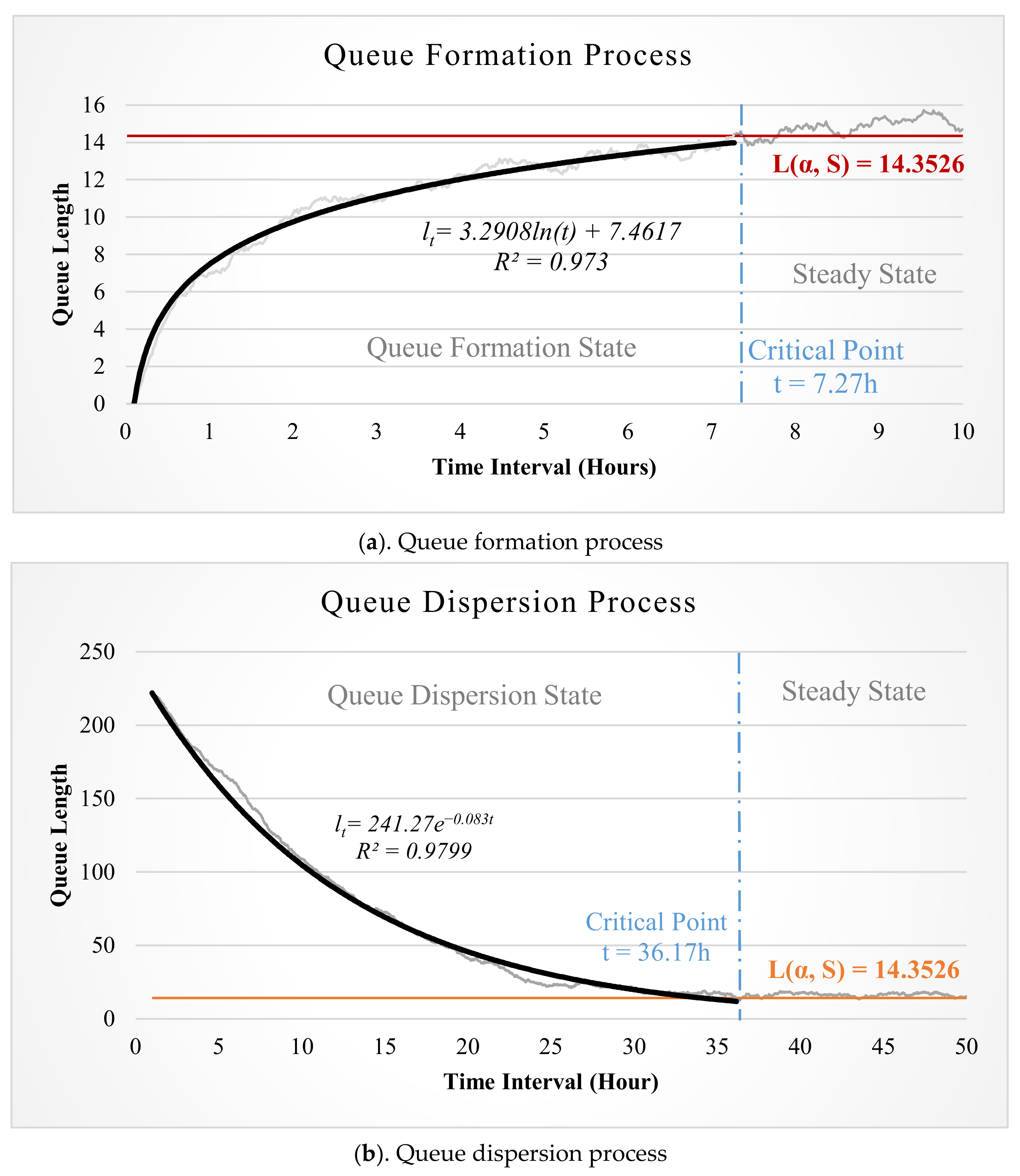
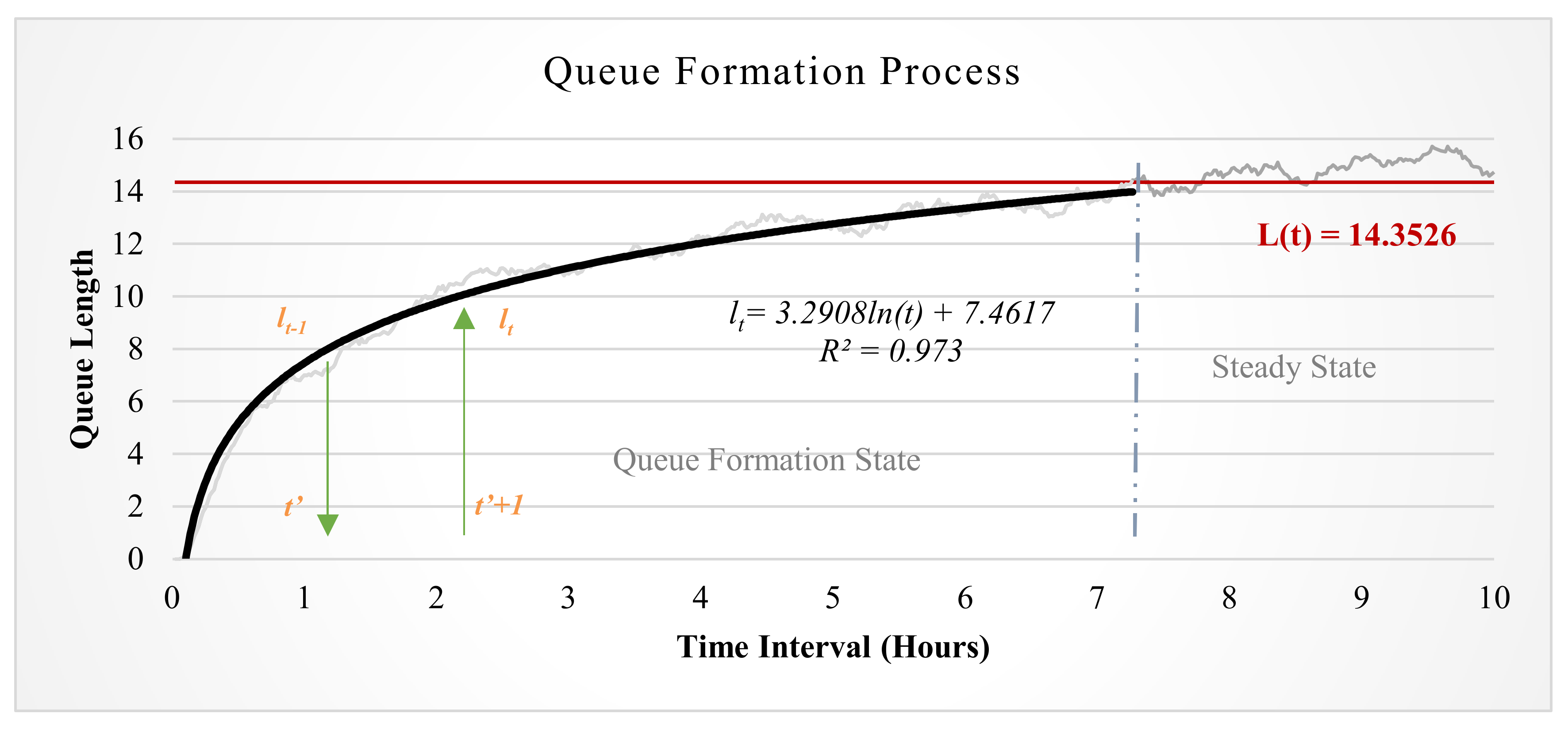
  • If $l_{t-1}<L_t$, it is at the queue formation state. Then, the regression models (see Equation (6)) developed for the queue formation state (given in Table 1) will be used to estimate the length of the queue at time interval t. Figure 3 shows the basic idea for this step. According to the value of $l_{t-1}$, the time needed for the queue length to reach $l_{t-1}$ can be derived by the regression model at first. Then, by adding 1 time interval, the current queue length $l_t$, can be estimated by the regression model. This can be expressed mathematically as follows:

    $$l_t^{queueformation}=a_1({\alpha }_t,S_t)ln\left(t^{\prime }+1\right)+b_1({\alpha }_t,S_t)$$

    (9)

    where:

    $$t^{\prime }=exp\frac{l_{t-1}-b_1({\alpha }_t,S_t)}{a_1({\alpha }_t,S_t)}$$

    In addition, since the estimated queue length will not exceed the steady length of the queue, then:

    $$l_t=min\{l_t^{queueformation},L_t\}$$
  • If $l_{t-1}>L_t$, it is at the queue dispersion state, and the regression models (see Equation (7)) developed for the queue dispersion state will be used to estimate the queue length at time interval t. Similarly, the current queue length, $l_t$, can be estimated according to the value of $l_{t-1}$, by the following equations:

    $$l_t^{queuedispersion}=a_2({\alpha }_t,S_t)exp\left[b_2({\alpha }_t,S_t)\left(t^{\prime }+1\right)\right]$$

    (10)

    where:

    $$t^{\prime }=ln\left(\frac{l_{t-1}}{a_2({\alpha }_t,S_t)}\right)/b_2({\alpha }_t,S_t)$$

    and

    $$l_t=max\{l_t^{queuedisperson},L_t\}$$

    (11)
  • If $l_{t-1}=L_t$, it is at steady state, and then, the steady queue length $L_t$ can be used for estimating $l_t$. Based on the modeling ideals described above, the overall model can be expressed mathematically as:

    $$l_t=\left\{\begin{array}{l}\left\{\begin{array}{l}min\{l_t^{queueformation},L_t\},l_{t-1}<L_t\\ L_t,\hspace{1em}\hspace{1em}\hspace{1em}\hspace{1em}\hspace{1em}\hspace{1em}\hspace{1em}\hspace{0.33em}\hspace{0.33em}\hspace{0.33em}{l}_{t-1}=L_t\\ max\{l_t^{queuedisperson},L_t\},\hspace{0.33em}\hspace{0.33em}\hspace{0.33em}{l}_{t-1}>L_t\end{array}\right.\\ l_{t-1}+{\lambda }_t-{\mu }_t\times S,\hspace{1em}\hspace{1em}if{\rho }_t\ge 1\hspace{0.33em}\hspace{1em}\hspace{1em}\hspace{1em}\hspace{1em}\hspace{1em}\hspace{1em}\hspace{0.33em}\end{array}\right.,\hspace{0.33em}\hspace{1em}if{\rho }_t<1$$

    (12)

    where ${\rho }_t=\frac{{\alpha }_t}{S_t}$, $l_t^{queueformation}$ is estimated by Equation (9), $l_t^{queuedispersion}$ is estimated by Equation (10), and $L_t$ is estimated by Equation (5).

4. Model Evaluation

To evaluate the model that was developed, a case study was conducted to compare the accuracy of the model with other existing methods, including the fluid flow model, the M/M/S queuing model, and the simulation-based regression model developed by Chen and Yang [5], which is referred to as Chen (2014)’s model. A simulation-based numerical experiment was conducted to derive the simulated truck queue length at a maritime terminal where the truck arrival rate and the gate service rate vary throughout the day. It was assumed that the hourly truck arrival rate increased from 35 to 45 during the first 10 h and decreased to 31 for the rest of the day. To compare with Chen (2014)’s model, the number of gate booths S and the service rate µ (number of trucks that can be served per hour) were set the same as in Chen (2014)’s model, i.e., S = 2 and µ = 40.8. Therefore, the system was oversaturated during a 9-h peak period (from 6th to 14th hour). The proposed modeling method was used in this case study, and the modeling results and the results of other existing models are presented in Figure 4. By comparing the simulated truck queue lengths with the queue lengths estimated by different models, the following key findings were obtained:

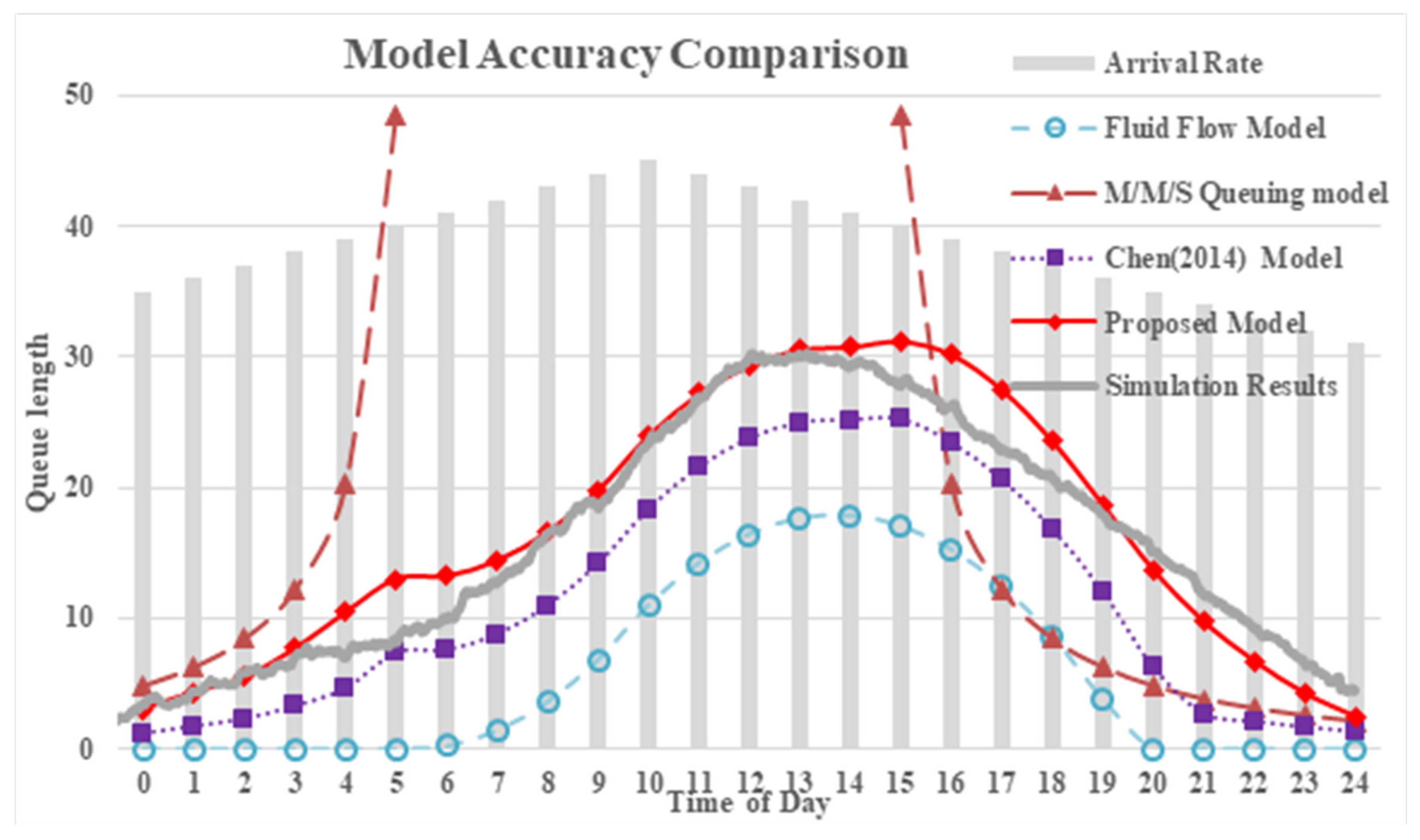
• Overall, the proposed state-dependent approximation method outperformed the other modeling methods regarding the accuracy of the estimation. Other models either underestimated or overestimated the queue lengths.
• The fluid flow model significantly underestimated the queue length because it neglected the random fluctuations in the arrival rate and the gate service rate.
• The M/M/s queuing model cannot be used in the oversaturation condition ($\rho$ > 1), and it significantly overestimated the queue length for the queue formation state and significantly underestimated the queue length for the queue dispersion state.
• Chen (2014)’s model had a comparable performance during the queue formation process. However, it significantly underestimated the queue length during the queue dispersion process because this process was not considered in the model.

5. Discussion

The proposed modeling method can estimate the truck queue length more accurately than the other four existing methods. It is because the truck queue length needs several hours to reach its steady-state and the developed model is the only model that can take account of both the queue formation and dispersion processes. In addition to the model estimation accuracy, the proposed model is more flexible and applicable than other models. First, it can be used for both undersaturated and oversaturated situations. This new method can accurately estimate the truck queue length caused by the short-term oversaturation during peak hours. Therefore, it will be useful for assessing the effectiveness of the countermeasures that are targeted at reducing the peak-hour congestion at marine terminals. Second, since the model estimates the truck queue length based on two input variables, i.e., traffic density ($\alpha =\lambda /\mu$) and the number of gate booths (S), it can be used for marine terminals that have different numbers of gate booths and different gate services rates.

In terms of the model applications, the developed model can be used for assessing the effectiveness of some countermeasures that reduce the terminal gate congestion by controlling the truck arrival rate (such as terminal appointment system), reducing the gate service time (such as using optical character recognition (OCR) technology and IT system) or increase the number of gate booths. Besides, it can be used as a sketching tool to quickly estimate the truck queue lengths to help design the scenarios for simulation-based port operation modeling. For example, the size of the buffer zone in the simulation model can be set according to the estimated truck queue lengths.

6. Conclusions

In this study, a state-dependent approximation method for estimating truck queue length at marine terminals was developed to fill the gaps in the existing methods. Based on the simulation of the truck queuing system, it was found that it takes several hours for the truck queue length to reach its steady state, and neglecting the queue formation (queue dispersion) processes will cause overestimation (underestimation) of truck queue length. To address this problem, the proposed method takes account of both the queue formation and dispersion processes into the truck queue length estimation. The model evaluation results showed that it can produce more accurate and robust estimates of the truck queue length than the existing methods. In addition, this new method can accurately estimate the truck queue length caused by the short-term oversaturation during peak hours. Therefore, it will be useful for assessing the effectiveness of the countermeasures that are targeted at reducing the peak-hour congestion at marine terminals. Furthermore, the developed model can be applied to estimate the customers’ queue at any service facility in the transportation and logistic industry where the customer arrival rate and service rate vary by time and system oversaturation conditions exist during peak hours.

In this study, the proposed model was evaluated based on the simulation experiment results. In the future, field data need to be collected at the maritime terminal gates to further verify the accuracy of the developed model. In addition, more research can be conducted on the application of the developed model to optimize some operational strategies, such as the terminal appointment system, to minimize the truck queue length at the terminal gates.

References

1. Giuliano, G.; O’Brien, T. Reducing port-related truck emissions: The terminal gate appointment system at the Ports of Los Angeles and Long Beach. Transp. Res. Part D Transp. Environ. 2007, 12, 460–473. [Google Scholar] [CrossRef]
2. Guan, C.Q. Analysis of Marine Container Terminal Gate Congestion, Truck Waiting Cost, and System Optimization. Ph.D. Thesis, New Jersey Institute of Technology, Newark, NJ, USA, 2009. [Google Scholar]
3. Chen, X.; Zhou, X.; List, G.F. Using time-varying tolls to optimize truck arrivals at ports. Transp. Res. Part E Logist. Transp. Rev. 2011, 47, 965–982. [Google Scholar] [CrossRef]
4. Green, L.; Kolesar, P. The Pointwise Stationary Approximation for Queues with Non-Stationary Arrivals. Manag. Sci. 1991, 37, 84–97. [Google Scholar] [CrossRef] [Green Version]
5. Chen, G.; Yang, Z.Z. Methods for Estimating Vehicle Queues at a Marine Terminal: A Computational Comparison. Int. J. Appl. Math. Comput. Sci. 2014, 24, 611–619. [Google Scholar] [CrossRef] [Green Version]
6. Yoon, D. Analysis of Truck Delays at Container Terminal Security Inspection Stations. Ph.D. Thesis, New Jersey Institute of Technology, Newark, NJ, USA, 2007. [Google Scholar]
7. Minh, C.C.; Huynh, N. Optimal design of container terminal gate layout. Int. J. Shipp. Transp. Logist. 2017, 9, 640–650. [Google Scholar] [CrossRef]
8. Grubisic, N.; Krljan, T.; Maglić, L.; Vilke, S. The Microsimulation Model for Assessing the Impact of Inbound Traffic Flows for Container Terminals Located near City Centers. Sustainability 2020, 12, 9478. [Google Scholar] [CrossRef]
9. Preston, G.C.; Horne, P.; Scaparra, M.P.; O’Hanley, J.R. Masterplanning at the Port of Dover: The use of discrete-event simulation in managing road traffic. Sustainability 2020, 12, 1067. [Google Scholar] [CrossRef] [Green Version]
10. Huynh, N.; Walton, C.M. Robust Scheduling of Truck Arrivals at Marine Container Terminals. J. Transp. Eng. 2008, 134, 347–353. [Google Scholar] [CrossRef]
11. Namboothiri, R.; Erera, A.L. Planning Local Container Drayage Operations Given a Port Access Appointment System. Transp. Res. Part E 2008, 44, 185–202. [Google Scholar] [CrossRef]
12. Karafa, J. Simulating Gate Strategies at Intermodal Marine Container Terminals. Master’s Thesis, University of Memphis, Memphis, TN, USA, 2012. [Google Scholar]
13. Fleming, M.; Huynh, N.; Xie, Y. Agent-based simulation tool for evaluating pooled queue performance at marine container terminals. Transp. Res. Rec. 2013, 2330, 103–112. [Google Scholar] [CrossRef]
14. Li, N.; Chen, G.; Govindan, K.; Jin, Z. Disruption management for truck appointment system at a container terminal: A green initiative. Transp. Res. Part D Transp. Environ. 2018, 61, 261–273. [Google Scholar] [CrossRef]
15. Azab, A.; Karam, A.; Eltawil, A. A simulation-based optimization approach for external trucks appointment scheduling in container terminals. Int. J. Model. Simul. 2020, 40, 321–338. [Google Scholar] [CrossRef]
16. Martonosi, S.E. Dynamic Server Allocation at Parallel Queues. IIE Trans. 2011, 43, 863–877. [Google Scholar] [CrossRef] [Green Version]
17. Chen, G.; Govindan, K.; Yang, Z.Z.; Choi, T.M.; Jiang, L. Terminal appointment system design by non-stationary M (t)/Ek/c (t) queueing model and genetic algorithm. Int. J. Prod. Econ. 2013, 146, 694–703. [Google Scholar] [CrossRef]
18. Dragović, B.; Tzannatos, E.; Park, N.K. Simulation modeling in ports and container terminals: Literature overview and analysis by research field, application area and tool. Flex. Serv. Manuf. J. 2017, 29, 4–34. [Google Scholar] [CrossRef]
19. Azab, A.E.; Eltawil, A.B. A Simulation Based Study of the Effect of Truck Arrival Patterns on Truck Turn Time in Container Terminals. In 30th European Conference on Modelling and Simulation (ECMS 2016); Curran Associates, Inc.: Red Hook, NY, USA, 2016; pp. 80–86. [Google Scholar]
20. Derse, O.; Gocmen, E. A Simulation Modeling Approach for Analyzing the Transportation of Containers in a Container Terminal System. Int. Sci. Vocat. J. 2018, 2, 19–28. [Google Scholar]
21. Preston, C.; Horne, P.; O’Hanley, J.; Paola Scaparra, M. Traffic modelling at the Port of Dover. Impact 2018, 2018, 7–11. [Google Scholar] [CrossRef] [Green Version]
22. Sharif, O.; Huynh, N.; Vidal, J.M. Application of El Farol model for managing marine terminal gate congestion. Res. Transp. Econ. 2011, 32, 81–89. [Google Scholar] [CrossRef]
Figure 1. Diagram of the quantity of fluid and time in the fluid flow queue (source: Martonosi, 2011).
Sustainability 13 02917 g001
Figure 2. Simulation results for an example scenario (S = 20 and α = 19).
Sustainability 13 02917 g002
Figure 3. Estimation of the Queue Length for the Queue Formation State.
Sustainability 13 02917 g003
Figure 4. Estimated Truck Queue Lengths by Different Models for the Case Study.
Sustainability 13 02917 g004